Estimation of Wastewater Discharges by Means of OpenStreetMap Data

Abstract

For the optimization of sewer networks and integration of water management in urban planning, estimations of wastewater discharges at a high spatial resolution are a key boundary condition. In many cases, these data are not available or, for reasons of data protection and company secrecy, the data are not accessible for research purposes. Therefore, procedures are needed to determine the volume of wastewater with high spatial resolution, based on freely accessible data. The approach presented here uses mainly OpenStreetMap (OSM) data, combined with a dataset of the German official topographic–cartographic Information System (ATKIS), to estimate the volume of wastewater on a building level. By comparison with daily values of the dry weather inflow at pumping stations and sewage treatment plants, it is shown that the method can generate realistic results, if target inflows exceed 50 m³/d. Difficulties due to the effect of commuting and the individual use of the buildings have to be considered, as well as data-quality issues in the OSM dataset. As an application example, the generated wastewater discharges are spatially joined with land-use plans. The resulting wastewater yield factors serve as input data for decision-support tools in urban water planning or modeling tasks.

1. Introduction

Sewage networks for the transport of wastewater from industrial, commercial, and residential areas to sewage treatment plants are essential elements of the water infrastructure. As the construction and maintenance of wastewater networks are cost-intensive, a large number of research projects are dedicated to the optimization of such infrastructures [1].

In recent years, the focus has been on the development of optimization algorithms for layout and component size of sewer networks [1,2,3,4]. Wastewater discharges as a main boundary condition for optimization are often regarded as “given” [1,3] without going into details in terms of data sources. In other works, the amount of wastewater is merely estimated, e.g., based on the drinking-water consumption of larger supply areas and provided with a peak factor [2]. Here, wrong assumptions about the amount of wastewater may lead to an oversized or undersized system [5].

In the work of Willuweit and O’Sullivan [6] a combination of models is used to simulate water demand, water supply, wastewater, and runoff in urban areas, under changing land-use and climate scenarios. In the water balance approach, it is assumed that the amount of wastewater produced corresponds to the domestic water consumption. To estimate the water demand, flows monitored in district metered areas are evenly distributed to cells of 4 ha size, using GIS software.

To determine the amount of wastewater inflow into existing drainage systems, the worksheet 118 [7] of the German Association for Water, Wastewater and Waste (DWA) recommends measurements of dry weather runoff with long measurement periods, if possible, in different seasons, as well as additional measurements in commercial, industrial, or tourist areas. However, the collection of data with a temporally and spatially high-resolution involves a great deal of effort. In addition, data protection and company secrecy restrict the availability of such datasets. Hence, procedures are needed to determine the volume of wastewater with high spatial resolution, based on freely accessible data.

A common approach to determine the domestic water use is by population figures. For instance, Schiller and Bräuer [8] present a method using population figures from official statistics, disaggregated by building footprints from ATKIS (official German topographic–cartographic dataset). The main part of their method is the classification of three settlement/municipality types and ten building types based on topographic geodata and building footprints from the ATKIS basic digital elevation model (DEM) with GIS tools. Building footprints and information about the use of buildings can also be derived from OpenStreetMap (OSM) datasets. Bakillah et al. [9] use points of interest (POI) from OSM as indicators for high or low population densities, to disaggregate population figures of the city of Hamburg into a grid (500 m² per grid cell). They then distribute the population of each grid cell proportionally to the OSM building footprint size within it. Kunze [10] uses building attributes stored in OSM data to describe the share of non-residential use in existing buildings. Fan et al. [11] derive different building types from semantic information and the shape of the building floor area in OSM.

OSM geodata are maintained and continuously expanded by the OSM community. This way of generating and collecting data is called volunteered geographical information (VGI) [12]. Since the data are collected by nonprofessionals, the preparation and quality assurance of VGI data, in general, and of OSM data, in particular, are much more demanding than of data collected specifically for a particular research question. A large number of articles is devoted to quality assessment and assurance at VGI in general [13,14,15,16,17,18,19]. Particularly for OSM building datasets, the data quality is the subject of various studies regarding completeness [20,21], building density [22], and accuracy of geometries [23]. Heterogeneity and incompleteness of the data is a common challenge. A higher data density and accuracy of OSM buildings in cities compared to rural regions can be explained by the number of local participants in the OSM project, which is generally larger in cities [15,16,24]. The same findings are noted for land-use data [16]. In addition, incorrect data collection by nonprofessionals is a common difficulty, as is the lack of metadata or the ability to verify data [17].

Nevertheless, VGI has proved to be a useful data source in many fields of application and scientific questions, since—as the word “volunteered” suggests—they are voluntarily made available to the public and, thus, the user does not have to spend any time on data collection. OSM data are freely available and may be used under the Open Database License [25]. Application examples for VGI are the mapping of flood hazards [26], disaster management [27], modeling of energy infrastructure [25,28], validation of land-use maps [29], or ecological monitoring [30]. The application of OSM data in urban-planning contexts has so far been investigated primarily in the field of transport infrastructure planning [31,32] and the analysis of settlement structures [8,33]. In the field of urban water management, the OSM road network was used to generate virtual wastewater networks [34,35]. The connecting element between settlement structure and sewage network was not considered in the mentioned work: wastewater from residential buildings, industry and commerce, or other uses that is transported to a treatment plant along the sewage network.

In this article, a method for the estimation of the wastewater volumes based on OSM data is presented. The parameters used for the calculations are optimized by comparing the estimated wastewater volumes in the catchment area of wastewater treatment plants (WWTPs) and sewage pumping stations (SPSs) with measured dry weather inflows. As a sample application, estimated wastewater discharges are spatially intersected with land-use plans, to develop a scenario-capable tool for the integral planning of settlement structural measures.

2. Materials and Methods

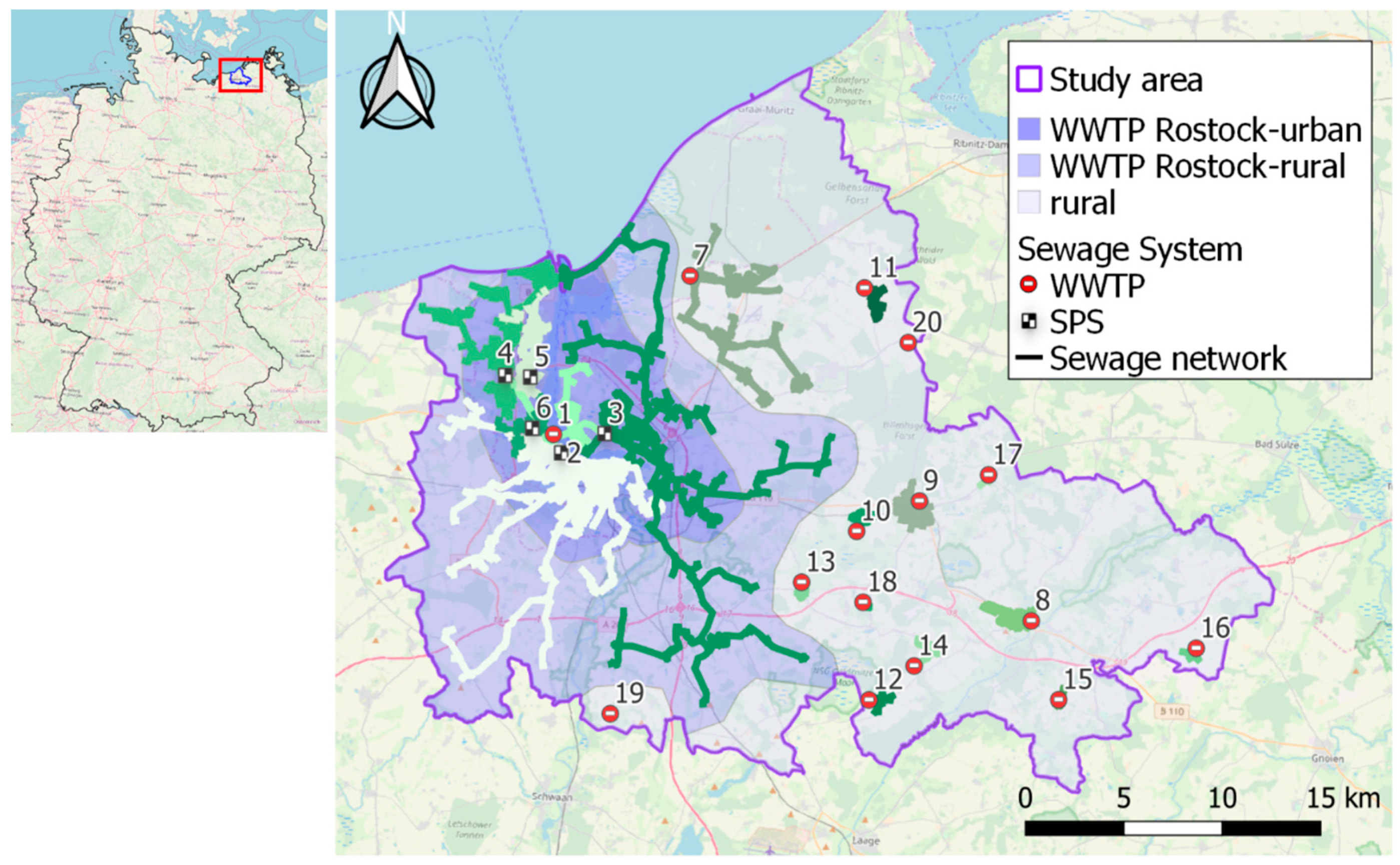
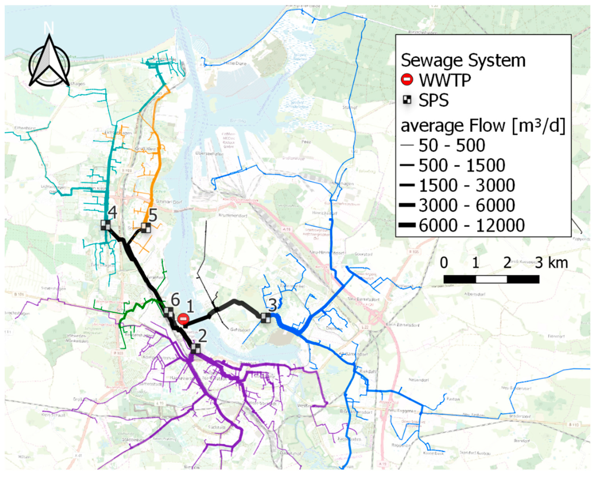
2.1. Study Area

The “Regiopolregion Rostock” is located in the northeast of Germany (see Figure 1, left). A regiopol region consists of a smaller large city with the surrounding rural region. Urban and rural areas differ in building types, infrastructure, land use, and population density [36], leading to a large heterogeneity concerning amount and variability of mass flows, such as wastewater [37]. The socioeconomic center of the area is the city of Rostock, with approximately 200,000 inhabitants. The communities in the surrounding area, by contrast, have a more village-like or small-town character. The area of responsibility of the Warnow Water and Wastewater Association (WWAV), purple boundary line in Figure 1) covers the entire urban area of Rostock with a sewer connection rate of 99.7%, as well as 29 municipalities in the south and east of the city. Wastewater treatment is mainly performed at the central wastewater treatment plant in Rostock (point 1 in Figure 1), with a capacity of 400,000 population equivalents (PE). Because of small slopes in the coastal region, wastewater is transferred to the central WWTP via 310 SPSs. With 14 further central sewage treatment plants in the association area, with capacities between 49 and 4999 PE, a fairly high connection rate of 87.6% is also achieved in rural areas. In addition, there are 1989 decentralized small sewage treatment plants (up to 49 PE) [38].

For the method presented here, building polygons and land-use polygons are obtained from the OSM provider Geofabrik (for Mecklenburg-Vorpommern: [39]). The dataset clipped to the study area contains 79,053 building polygons. Basic elements in OSM are points/”nodes” (points of interest or centroids of surfaces), open or closed lines/”ways”, and “relations” (relationships between objects, such as groups of objects). All OSM elements get their properties from attributes/”tags”, each consisting of a key and a value [40]. Polygons are constructed by closed lines with the attribute “area=yes” and with certain tags like “building=*” or “landuse=*” (“*” being a particular attribute), which are assigned exclusively to areal elements. In OSM, buildings, in particular, are assigned by the tag “building=*”. For example, a building is already clearly identified by “building=yes”, but it can also be more precisely labeled by other values (e.g., “building=hotel”). However, an element declared as a building could also get the property “hotel” by “tourism=hotel”. For the assignment of OSM tags, the OSM Wiki website provides a multitude of hints and examples. These can be regarded as a guideline more than a fixed set of rules. New tags can be proposed, changed, and discarded by the OSM community [40].

Additional information on land use, as well as population figures of municipalities and municipal boundaries, is taken from official data (e.g., ALKIS, provided by regional administrations [41]). A digital map (shapefile) of the sewage network and measured values of the daily inflow to WWTPs and SPSs from the regional wastewater association WWAV are used for the optimization process.

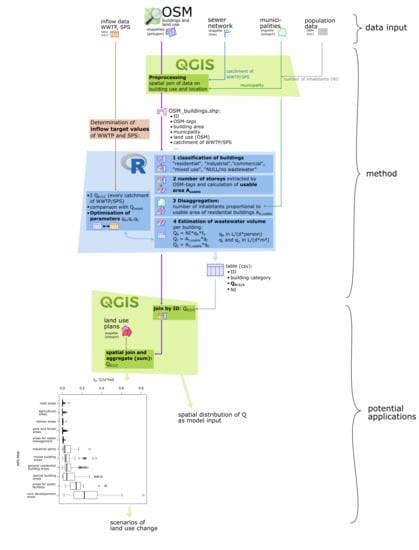
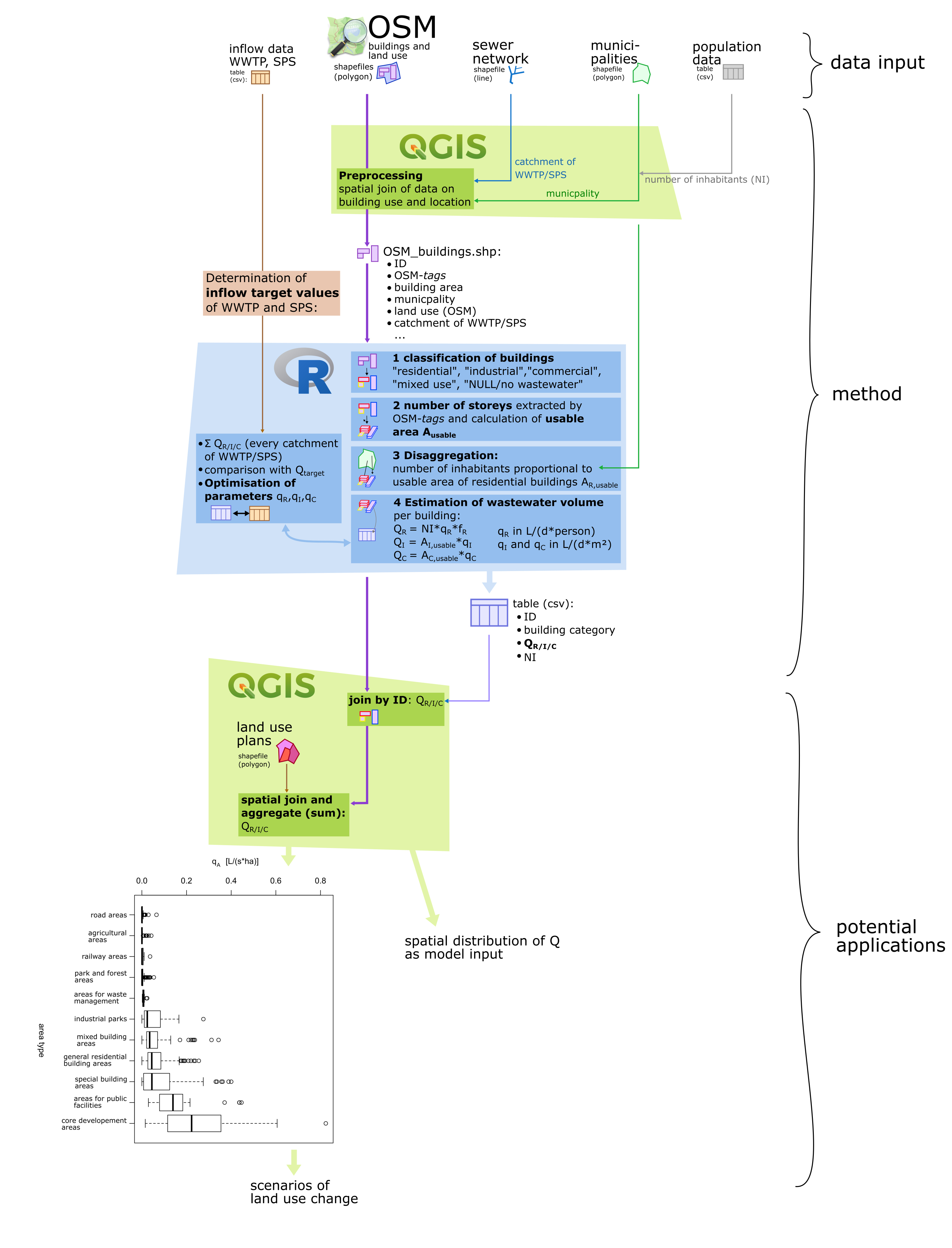
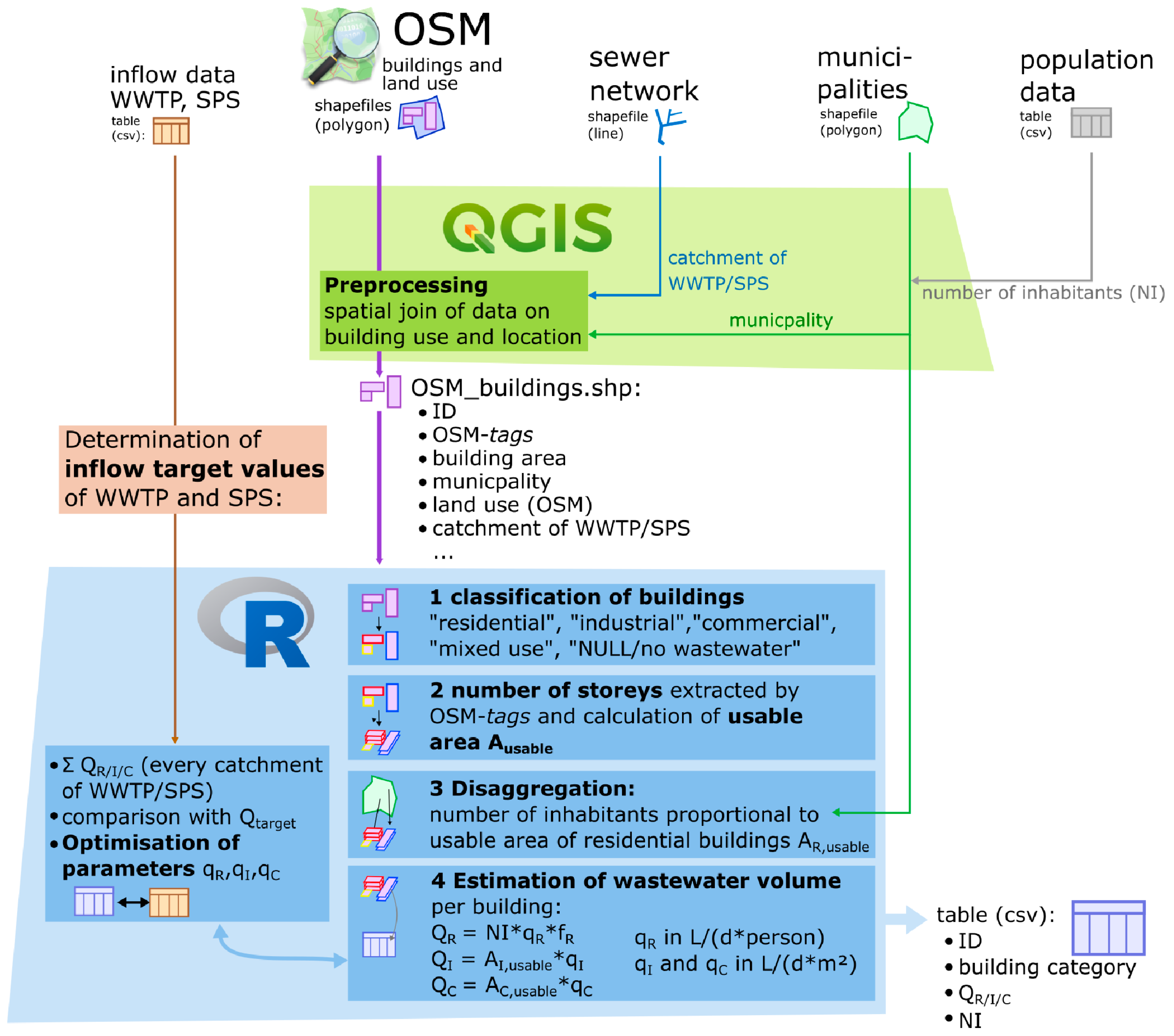
2.2. Generation of Wastewater Volume per Building

GIS software is used to link OSM building polygons with information on land use (OSM: land use, ALKIS) and location (municipality, WWTP catchment area) by spatial intersection. The further calculation of the wastewater volume is performed in four steps using R scripts [42]. An overview about the method is illustrated in Figure 2.

According to the wastewater discharge components described by the German DWA worksheet 118 [7], buildings are classified into “residential buildings”, “industrial buildings”, and “commercial buildings” in step 1. Buildings that combine different uses (e.g., retail trade with living space on the floors above), are assigned to the type “mixed-use buildings”. Buildings that (presumably) do not discharge wastewater into the network, are assigned to the “NULL” category. The classification process is carried out by various attributes:

• OSM tags of the buildings, e.g., “building”, “leisure”, and “amenity” (see [11]). Some examples are shown in

  Table 1. Used OSM-tags (abstract) for the classification of buildings.

  Residential	Commercial	Industrial	NULL
  Apartments	airport_terminal	cowshed	abandoned
  Detached	commercial	Dock	allotments
  Dormitory	doctor	Farm	cabin
  House	hall	greenhouse	carport
  Private	hospital	industrial	collapsed
  Residential	hotel	manufacture	container
  Semi	kiosk	Mill	construction
  semidetached_house	museum	Stable	garages
  Terrace	office	Storage	gasometer
  Yes	public	Sty	ruins
  …	…	…	…

  .
• OSM tags of land-use polygons on which a building is located.
• If none of the former is stated: land-use information derived from ALKIS.

In step 2, the number of floors is—if available—directly extracted from OSM tags (“levels”), derived from the building height (“building:height”) or estimated on the basis of the usage class of the building. The usable area of a building is calculated by multiplying the floor area with the number of floors, less 5% as unusable area. The number of inhabitants (NI) of every municipality is then disaggregated proportionally to the usable area of each of its residential or mixed-use buildings (step 3).

Step 4 of the algorithm is the calculation of wastewater discharges per building by Equation (1) (residential buildings), Equation (2) (industrial buildings) and Equation (3) (commercial buildings). For mixed-use buildings, the Equations (1)–(3) are employed proportionately.

Q_R = NI × q_R × f_R,

(1)

Q_I = A_I,usable × q_I,

(2)

Q_C = A_C,usable × q_C,

(3)

Discharge rates for residential (q_R) (in L/(person*d)), commercial (q_C), and industrial buildings (q_I) (each in L/(m²*d), related to the building footprint area) are determined by the optimization algorithm described in the following section. It is assumed that a large proportion of the inhabitants of the surrounding municipalities does not work at their place of residence. As a result, a part of the domestic wastewater is not produced in these municipalities, but is already contained in the wastewater from commercial buildings. This fact is taken into account in the calculation by a “rural factor”, f_R (a fixed value for every municipality; between 0.6 and 1), depending on the population density of the municipality.

2.3. Optimization of Parameters

The wastewater volume, Q_catchm,_n which is generated in the catchment area, A_n, of a sewage treatment plant or a pumping station with the number, n, consists of domestic, industrial, and commercial wastewater:

Q_catchm,n = ∑Q_R,n + ∑Q_I,n + ∑Q_C,n,

(4)

Catchment areas of pumping stations and sewage treatment plants are defined along the sewage network in the area of responsibility of the WWAV (see Figure 1). For this purpose, buildings are linked to the nearest sewer by GIS queries. Flow paths are determined by using routing scripts from the QGIS plugin “WaterNetAnalyzer”, which was developed by the authors within this study [43].

The amount of wastewater, Q_catchm, generated in the catchment area of 15 WWTPs (Points 1 and 7–20 in Figure 1) and 5 main SPS (Points 2–6 in Figure 1) are compared with corresponding measured values of the daily inflow. The first quartile of dry weather inflows (1 January 2017 to 31 December 2018) is selected as the target value for each of the five main pumping stations and the WWTPs in the study area. Dry weather inflow is assumed, if the total precipitation measured on the day itself and on the previous day is below 0.1 mm/d. Where daily values of the inflow are not available, the average annual inflow of wastewater (2013–2017) to small WWTPs converted to a daily value is used as a target. The parameters q_R, q_I, and q_C are optimized by minimizing the deviation of the generated wastewater quantities from the target value for (Equations (5) and (6)):

min ∑ (Q_target,n − Q_catchm,n)²

(5)

Replacing Q_catchm,n in Equation (5) with Equations (1)–(4) equals the following:

min ∑ (Q_target,n − (∑NI_catchm,n × q_R × f_R + ∑A_{I,usable,catchm,n} × q_I + ∑A_{C,usable,catchm,n} × q_C))²

(6)

Optimum parameter combinations are determined using the R function “optim()” with the Nelder-Mead method [44], and the R function “lm()” for linear regression. The values used for optimization are presented in detail in

Table A1. NI = Number of inhabitants in the catchment; NI*f_R = NI multiplied with rural factor; A_R = residential building area; A_I = industrial building area; A_C = commercial building area, 1st Q. DW = 1st quartile of dry weather inflow to SPS or WWTP; Mean DW = mean of dry weather inflow to SPS or WWTP; LTA WW = long-term average of wastewater inflow to WWTP (see Section 2.3, Optimization of Parameters).

N	NI	NI*fR	AR (m²)	AI (m²)	AC (m²)	1st Q. DW (m³/d)	Mean DW (m³/d)	LTA WW (m³/d)
1	234,844	234,372	14,365,079	1,660,316	5,458,696	35,947	38,964	-
2	101,706	101,769	6,194,405	371,115	2,497,618	16,034	17,764	-
3	47,755	47,373	3,133,414	900,494	1,079,482	7501	8080	-
4	52,353	52,353	3,136,566	108,951	915,023	6498	7090	-
5	22,470	22,470	1,296,892	142,960	426,274	4189	4329	-
6	5549	5549	319,759	114,006	480,849	1338	1654	-
7	4629	4568	399,937	19,677	74,456	612	706	-
8	2880	2880	199,243	39,818	20,960	391	439	-
9	3238	3022	294,551	33,333	12,372	n.a	n.a	306
10	535	499	49,360	0	33,654	n.a	n.a	176
11	720	624	109,380	0	0	57	73	-
12	250	200	45,851	0	449	28	34	-
13	343	320	27,872	5271	8046	26	34	-
14	212	170	40,671	179	7974	26	30	-
15	105	77	15,540	4201	0	13	15	-
16	148	118	21,999	5111	771	n.a	n.a	10
17	162	151	14,736	0	0	6	8	-
18	100	93	9054	222	0	4	5	-
19	40	37	3211	0	496	n.a	n.a	3
20	48	42	7113	0	0	4	4	-

(Appendix A).

2.4. Application Example: Aggregation at LUP Level

Land-use plans (LUP) represent the intended urban development of a municipality. They are an essential tool for the integral planning of structural settlement measures in regiopol regions. A catchment yield factor, q_LUP,i (in L/(s*ha)), is derived for each subarea, i, of the LUP by spatially joining the estimated wastewater volume in GIS with the LUP of the City of Rostock (see Figure A1, Appendix C). For this purpose, wastewater discharges are aggregated in every LUP subarea and divided by its area A_LUP (Equation (7)).

q_LUP,i = ∑Q_LUP,i / A_LUP,i

(7)

The range of the catchment yield factors sorted by types of land use (e.g., residential area, mixed-use area, etc.) can be used in planning scenarios. For example, the effect of a planned industrial park on a sewage network can be investigated in models by multiplying its intended area with the median catchment yield factor of industrial areas.

3. Results and Discussion

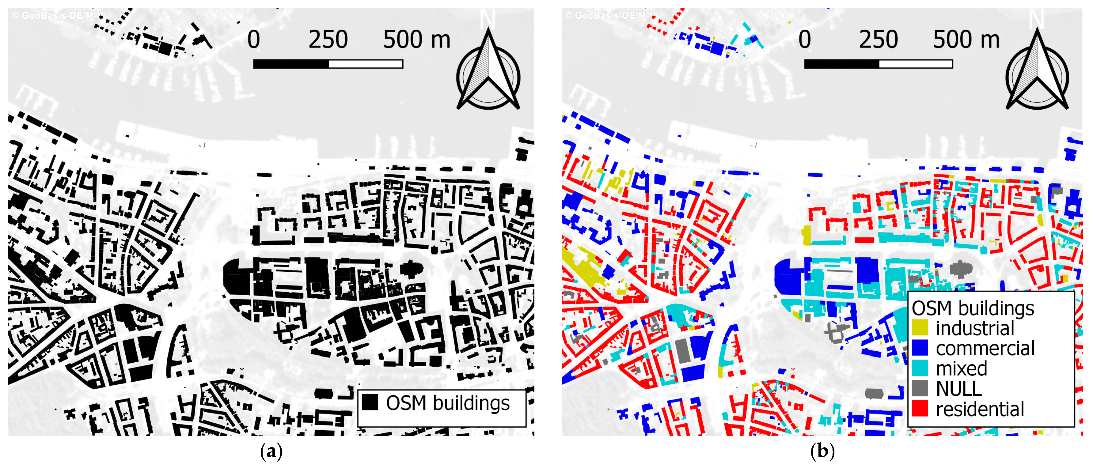
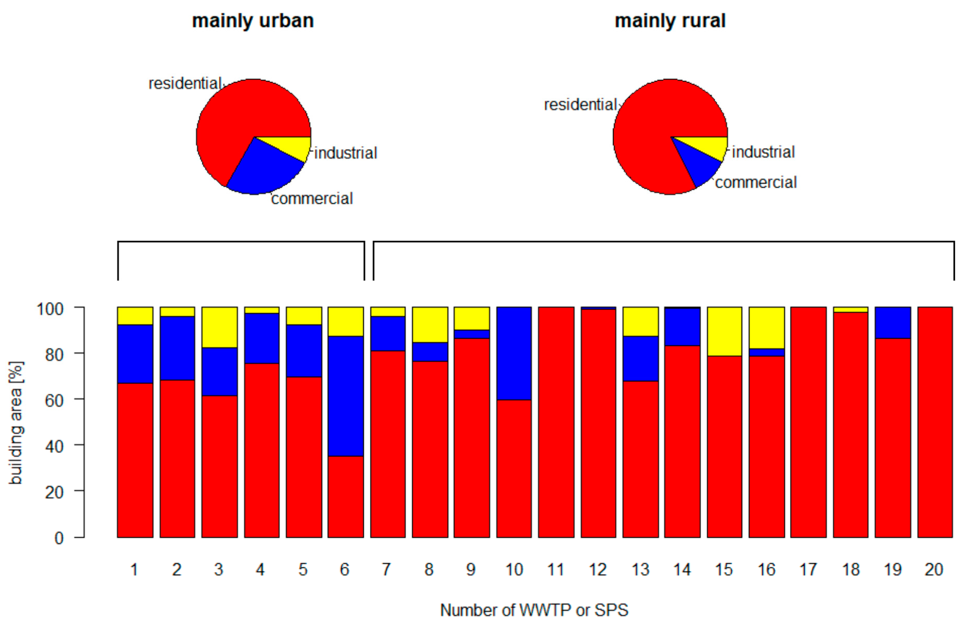
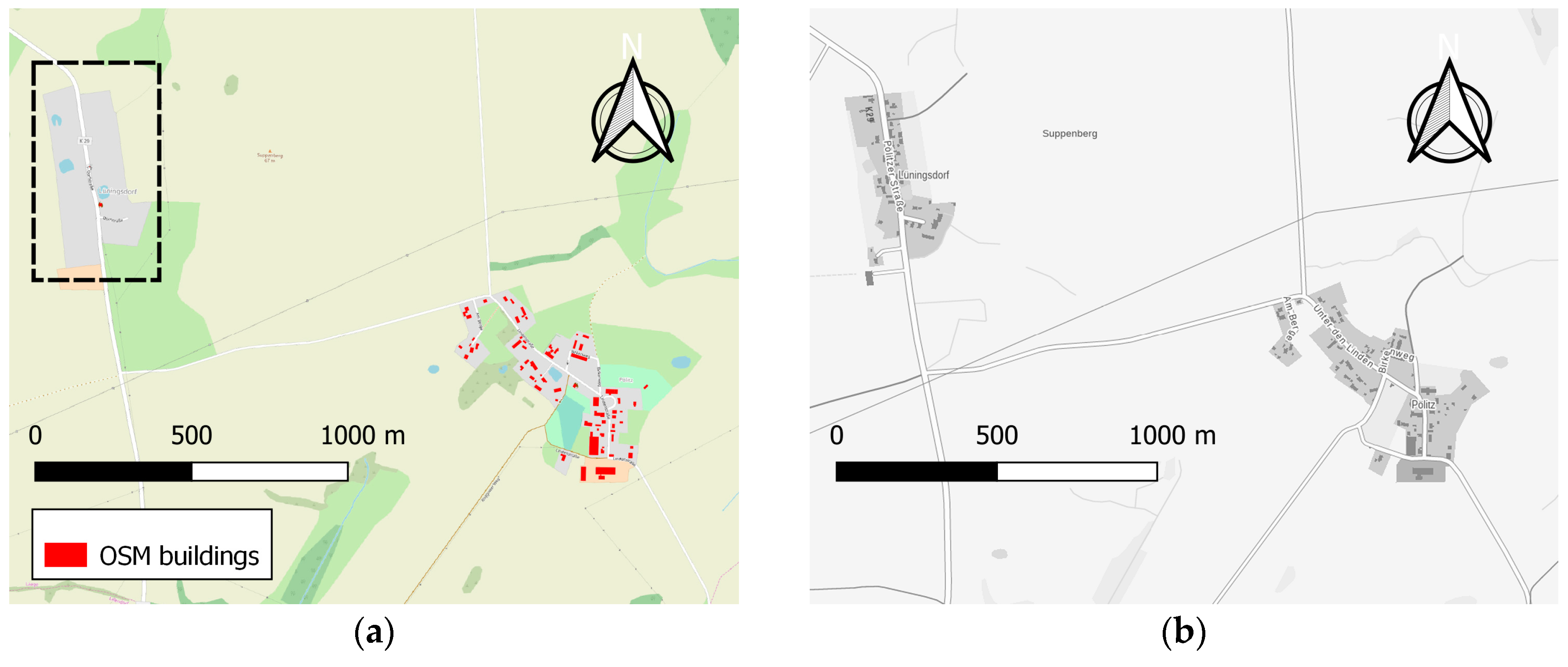
3.1. Classification of Buildings

The classification of the buildings into the mentioned categories is based on OSM tags and information on real land use from ALKIS data. Figure 3 shows the result of the classification in the inner-city area of the city of Rostock.

In the catchment of WWTP Rostock, the share of residential space is 67%. Moreover, 25% of the building areas are identified as commercial, and 8% are industrial areas. However, the distribution of the area categories also varies within the urban area (cf. Figure 4). In the catchment area of the SPS at point 6, the share of residential areas is only 35%. In contrast, 75% of the building areas are categorized as residential in the catchment of the SPS at point 4, where larger multistory blocks of flats are located. In the rather rural part of the study area, “residential” accounts for an average of 82% of the building areas, 11% are commercial and 7% are industrial building areas. Absolute values for each area type are provided in Table A1 (Appendix A).

An essential element of uncertainty is the unknown completeness and correctness of the OSM building polygons. Götz and Zipf [45] estimated that, at the time of their investigation only approximately 30% of all building geometries in Germany are recorded in OSM. They expected that continuous contributions of the OSM community would lead to an increasing percentage here, up to 90% within a few years. Even without a more precise evaluation, it is assumed that this figure will not yet be reached in the study area, as in certain villages, hardly any buildings have yet been marked (cf. Figure 5). A large number of missing building geometries can be expected in the rural municipalities [20]. A comparison of OSM buildings with official cadastral data can help to identify missing geometries here [21]. Irrespective of this, the OSM dataset for the city of Rostock is very extensive, as the Cadastral Office of Rostock donated a building dataset to the OSM project in 2009, including information on building height and use [20]. Moreover, the number of buildings in OSM is steadily increasing. Compared to an OSM dataset of the same research area obtained two months before, the dataset used here contains already 7695 more (which corresponds to +4.7%) building polygons.

Not only completeness (in terms of the number of buildings) but also the number of tags assigned in rural areas in the study area is considerably lower. Properties such as the building height or the number of floors are mainly available in the urban part of the study area. About 82% of the buildings are only marked by the tag “building = yes” [47]. To deal with this lack of information about building attributes, the layer can be intersected with land-use data [25]. In the current version of the method presented here, the attribute “land use” from the ALKIS dataset is also utilized to categorize buildings. In cases where even this information is not available, the category “residential buildings” is chosen, which applies to 0.6% of the buildings, mostly in rural areas. In this way, the algorithm classifies all buildings reliably into wastewater categories. At the same time, however, agricultural buildings in rural areas—stables, halls, etc.—are wrongly identified as residential buildings, when OSM tags are missing. As a result, the disaggregation of the population per municipality distributes the inhabitants among too many houses. The classification process could be improved by similarity measurements of building footprints, e.g., as described by Fan et al. [11], or by interpreting buildings and related “points of interest” [29].

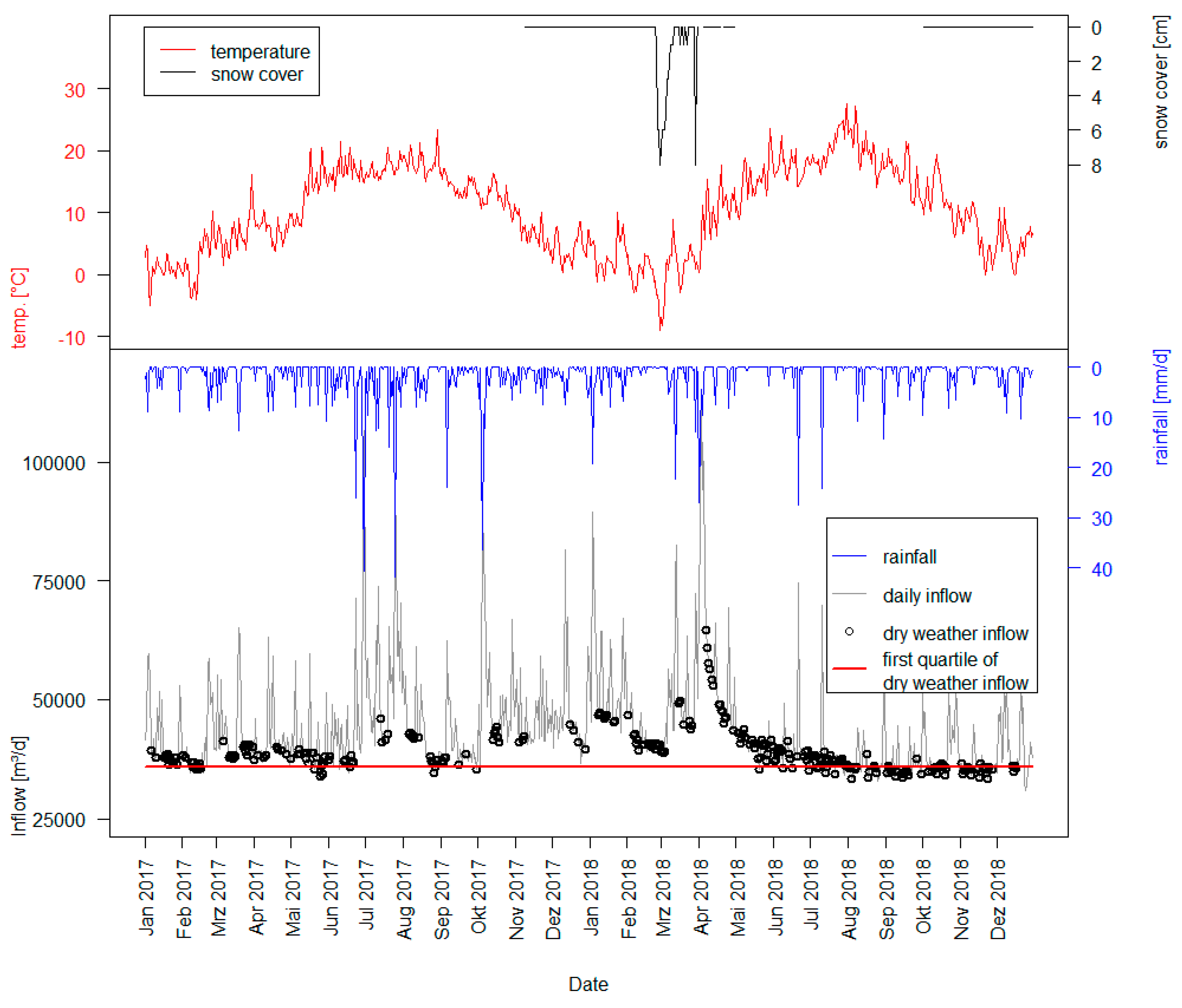
3.2. Determination of the Inflow Target Value

A critical point of the method is to find suitable target values for the calibration of the discharge rates q_R, q_I, and q_C. In the approach presented here, daily measurements of wastewater inflow to treatment plants and pumping stations are used. Since the volume of domestic and commercial wastewater is subject to daily fluctuations, the absolute minimum cannot be the target value. In this study, dry weather inflow is assumed if rainfall on the day itself and on the previous day is below 0.1 mm/d. Figure 6 shows the inflow to a pumping station at such conditions. In the periods from July 2017 to September 2017 and October 2017 to February 2018, high precipitation is recorded, which is the cause of higher water inflows to sewage treatment plants and pumping stations (see Figure 6). In general, the year 2017 can be classified as high in precipitation with 739 mm compared to the long-term average of 616 mm (1981–2010, calculated by precipitation data from the German national meteorological service (DWD) [48]). Presumably, due to the finely branched Rostock sewage network, which extends from the urban area to the suburbs and surrounding villages, rainfall events that occurred more than two days before are wrongly detected as dry weather inflow. Additionally, unavoidable infiltration of stormwater into separate drainage systems leads to higher inflows. Groundwater infiltration is likely to occur, as groundwater levels are generally high in many parts of the study area. Another issue that has to be considered here is extraneous water and snowmelt infiltration into the sewer system [49]. This is the case in March 2018 to April 2018. The mean value of the dry weather runoff is increased by such events and is therefore unsuitable as a target inflow value. To take the mentioned conditions into account, the first quartile of the dry weather inflow at sewage treatment plants and pumping stations is chosen as the target value. Other target values and approaches to determine them may be more suitable for other study areas. For example, wastewater volumes can be compared to drinking water intake in a first step. This can be used to exclude inflow values influenced by rainfall infiltration. Alternatively, hydrograph separation could be used to distinguish between wastewater flows and stormwater flows [50]. Where seasonal changes in wastewater inflow are high, the selection of separate target values for optimization for each season might be beneficial. To avoid misinterpretation of seasonal changes caused by single extreme events, the evaluation of time series longer than two years is recommended.

3.3. Parameter Optimizing Process

The two optimization methods result in similar parameter combinations, both for the optimization on the basis of the wastewater treatment plant inflows and the pumping station inflows. Since the catchment areas of the pumping stations are mostly located in the urban area and those of the sewage treatment plants (with the exception of the central sewage treatment plant Rostock) cover the rather rural area, differences in the optimized parameters q_R, q_I, and q_C (cf.

Table 2. Result of the parameter optimizing process.

Optimization Method	qR L/(person*d)	qC L/(m²*d)	qI L/(m²*d)	Area
Linear regression	80.1	2.7	1.5	WWTPs without central WWTP Rostock/ mainly rural area
Nelder–Mead	61.5	3.1	2.9
Linear regression	93.6	2.4	0.6	Pumping stations/mainly urban areas
Nelder–Mead	93.6	2.4	0.6
Linear regression	93.0	2.4	0.6	WWTPs including the central WWTP Rostock (entire study area)
Nelder–Mead	93.1	2.4	0.6

) can be attributed to settlement structural conditions. The estimated amount of wastewater, q_R, per inhabitant for parameter optimization is between 61.5 and 93.6 L/d, depending on the optimization method and the target values considered. The lower values are obtained for rural areas. As residential use is the main source of wastewater in the study area and the per capita volume of wastewater of 93 L/d matches the average drinking water consumption of 93.8 L/(person*d) indicated by the WWAV in 2017 [38], the parameter set optimized for the entire study area is chosen for further calculations:

• q_R = 93.0 L/(person*d);
• q_C = 2.4 L/(m²*d);
• q_I = 0.6 L/(m²*d).

The optimized parameter, q_C, for commercial buildings varies between 2.4 and 3.1 L/(m²*d). For industrial buildings, the optimization result of the parameter q_I is 0.6 to 2.9 L/(m²*d). Both q_C and q_I are higher in the rural part of the study area. These findings are explained by the classification process (cf. Figure 2, step 1). The algorithm identifies large production halls with presumably low wastewater output as industrial buildings in the urban area of Rostock, while agricultural buildings with presumably higher wastewater output (e.g., stables) are classified as “industrial” in rural areas. Accordingly, the actual amount of wastewater per m² in rural industrial buildings would also be higher than in urban industrial buildings (e.g., production halls), which is reflected in a higher optimized q_I.

Although a part of the drinking water in rural areas is not returned to the sewage network (e.g., for the irrigation of plants in gardens and dwellings) 61.5 L/(person*d) is too low, compared to the average consumption. There are several possible explanations for the low q_R value in rural areas. The effect of missing or incorrectly assigned buildings in the OSM dataset, as well as the effect of commuting, has to be considered. A large proportion of the rural population’s wastewater may be produced at the workplace in urban areas, so an adjustment of f_R is needed. In addition, with this factor, the settlement structure of different localities within a municipality is not taken into account so far. A small village with residential development next to a larger village with business parks (and accordingly jobs) in the same municipally is therefore evaluated equally. Here, further work is needed to establish parameters which can better represent this heterogeneity.

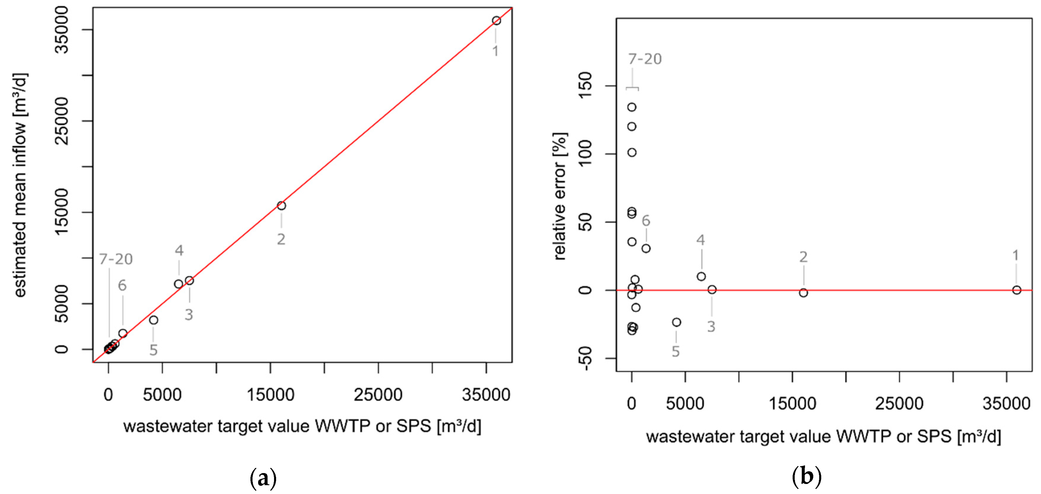
3.4. Calculated Wastewater Volume

The comparison of the calculated wastewater inflow with the daily values of dry weather inflow at SPSs and WWTPs shows that the method can generate realistic values mainly in urban areas (cf. Figure 7a, numbers 1–6). Here, the maximum relative error is 31%. The estimated wastewater volume of the central WWTP of Rostock (number 1) is 35,992 m³/d, which differs by 0.1% from the target value of 35,947 m³/d. Moreover, WWTPs in rural areas show relative errors less than 30% if target inflows exceed 50 m³/d. The estimated volume at WWTP number 8 is 341 m³/d, with 391 m³/d set as the expected value. WWTPs with a target inflow smaller than 50 m³/d can have large relative errors. For example, the estimated quantity of 14 m³/d at sewage treatment plant number 17 is more than twice the estimated value of 6 m³/d. An overview about all values is provided in

Table A2. Q_target = wastewater target value, Q_gen = generated wastewater inflow by OSM buildings, Err = absolute error; Rel. Err = relative error.

N	Qtarget (m³/d)	Qgen (m³/d)	Err (m³/d)	Rel. Err (%)
1	35,947	35,992	45	0.1
2	16,034	15,734	−300	−1.9
3	7501	7537	36	0.5
4	6498	7153	655	10.0
5	4189	3206	−983	−23.5
6	1338	1748	410	30.7
7	612	617	5	0.8
8	391	341	−50	−12.7
9	306	330	24	7.8
10	176	128	−48	−27.2
11	57	58	1	1.8
12	28	20	−8	−29.6
13	26	52	26	101.1
14	26	35	9	35.5
15	13	10	−3	−26.6
16	10	16	6	57.8
17	6	14	8	134.4
18	4	9	5	120.2
19	3	4	−1	3.3
20	4	5	1	55.9

(see Appendix B).

It must be borne in mind that the target value (1st quartile of dry weather inflow) is a parameter defined ad hoc which represents an assumption about the true average inflow in dry weather. In addition, the calculation with a single set of mean discharge rates q_R, q_C, and q_I cannot reflect the individual use of a specific building. For example, individual behavior of water consumption will lead to overestimations or underestimations if catchments are small. Furthermore, in sewage treatment plants with a smaller catchment area in rural areas, only a few missing or incorrectly allocated buildings have a negative effect on the calculated result. Hence, the relative error related to the target value is smaller, the larger the catchment area of the sewage treatment plant or pumping station (cf. Figure 7b).

Using disaggregation procedures as an example, Schiller and Bräuer [8] also argue that the individual error is greater the higher the level of detail. In the case of values generated on a building level, the error range is largest. The calculated result should therefore be aggregated on the largest possible reference level according to the planning task. For the drainage planning, the mentioned study proposes the level of districts or “solitary settlement units”. In the application example described here, the spatial resolution of LUP is chosen, which corresponds the proposed aggregation level by Schiller and Bräuer [8].

3.5. Application Examples LUP and Urban Wastewater Management

As described in Section 2.4, yield factors for every type of land use in LUPs are derived by a spatial join and aggregation process, using QGIS. The combination of land-use types and wastewater discharges enables illustrating the effect of land-use change in modeling future scenarios.

The largest wastewater yield factors (Figure 8) are related to the LUP types “areas for public facilities” and “core development areas” and (medians: 0.14 to 0.22 L/(s*ha)). Industrial parks, mixed building areas, residential areas, and special building areas are in the middle range of yield factors (medians: 0.05 to 0.07 L/(s*ha)). In the work of Willuweit and O’Sullivan [6], three land-use types are distinguished in the urban area of the Dublin region: For “medium dense to continuous dense urban fabric/commercial”, a value of 0.48 to 0.50 L/(s*ha) is estimated. For the category “sparse and discontinuous urban fabric/residential”, 0.14 to 0.16 L/(s*ha) is calculated, and 0.10 to 0.14 L/(s*ha) for cells of the land-use type “industrial”. Compared to the region of Rostock, the higher values cited here presumably result from a higher per capita water use. The water demand of the population of approximately 1.5 million in the Dublin Region Water Supply Area is 550*10⁶ L/d, which corresponds to 367 L/(person*d).

The DWA worksheet A 118 [7] recommends using 0.2 to 0.5 L/(s*ha) for choosing the component size of sewer networks in commercial and industrial areas for companies with low water consumption and up to 1.0 L/(s*ha) for companies with medium to high water consumption, referring to the catchment area connected to the sewage system. These values are higher than the calculated ones (see Figure 8), as they represent an (hourly) maximum instead of daily mean values. However, deriving the variability of wastewater discharge from OSM data or other VGI could be a subject of future research.

In Figure 8, wastewater is also “produced” on road areas, agricultural areas, park and forest areas, and areas for waste management. This can be due to incorrectly classified buildings or inaccurately drawn LUP areas. On the other hand, e.g., road areas actually contribute to the volume of wastewater, as tram depots or ticket counters are located in these areas.

The GIS-based approach to accumulate generated wastewater along a sewer network allows the estimation of the actual flows (see Figure 9). With the same approach, wastewater flows can be represented in future urban and regional planning variants. Possible applications are decision support systems for the construction or reconstruction of drainage systems on a conceptual level.

In the rural structured part of the study area, phosphate inputs from wastewater treatment plants into rivers are investigated [51]. When merging decentralized small wastewater systems into a central system, it is worth considering a fourth treatment stage to reduce the input via the treated wastewater. In order to determine the technological optimization potential, the amount of wastewater to be treated is the central data basis, in addition to the sewer system itself and equipment of the wastewater treatment plants.

On the other hand, especially in developing countries, the construction and maintenance of large sewerage networks and cost-effective wastewater treatment are a challenge. With the help of spatially differentiated wastewater data, decentralized wastewater concepts can be created in addition to existing systems, which enable the wastewater treatment and reuse close to the source [52].

4. Conclusions

The method introduced here represents an instrument to estimate discharges of wastewater from domestic, commercial, and industrial use on a high spatial resolution. The approach adds a new application for VGI to the existing methods. Using OSM as the main data source makes the method transferable to other regions. Where quality issues of OSM building data generate uncertainty, especially in rural regions, additional data from different sources, e.g., authoritative data, may be used to identify missing buildings. To achieve higher accuracy in the classification process, OSM buildings data could be enhanced with POI from OSM, or an analysis of shape and size of building footprints could be applied.

For the calibration of the discharge rates q_R, q_I, and q_C, finding suitable target values is an essential step. Extraneous water, such as groundwater infiltration through leakages and rainwater or snowmelt infiltration into the sewage system, leads to temporarily high discharge rates, which increase the difficulty of finding a target value for the inflow. As this is a crucial step of the method, different approaches for the determination should be tested in future research, e.g., hydrograph separation or calibration with consumption rates of drinking water. Where long-term series of inflow to WWTPs and SPSs are available, the variability of wastewater discharges can be estimated by minimum and maximum values for different spaces of time. Seasonally varying target values derived in this way could improve the accuracy of the results, especially for small catchment areas of WWTPs. The method shown here, which uses one target value per WWTP or SPS, can be applied when inflow data sources are limited.

Wastewater discharges aggregated along the sewer networks in the study area generate realistic inflows to WWTPs and SPSs, which differ by a maximum of 31% from the target inflow when this value exceeds 50 m³/d. In small catchments, individual behavior of water consumption may lead to overestimates or underestimations. Here, the integration of peak factors to represent variability of wastewater discharges could improve the estimation. The estimated values cannot replace time-consuming measurements. However, the method can fill the gap of input data for model-building and urban water management, especially for research purposes, when measured data do not exist or their availability is legally restricted. By intersection of discharges with land-use plans, wastewater yield factors are derived as a scenario-capable tool, which enables us to simulate the effect of land-use change in modeling future scenarios.

References

1. Navin, P.K.; Mathur, Y.P. Layout and Component Size Optimization of Sewer Network Using Spanning Tree and Modified PSO Algorithm. Water Resour. Manag. 2016, 30, 3627–3643. [Google Scholar] [CrossRef]
2. Zhao, W.; Beach, T.H.; Rezgui, Y. Optimization of Potable Water Distribution and Wastewater Collection Networks: A Systematic Review and Future Research Directions. IEEE Trans. Syst. Man Cybern. Syst. 2016, 46, 659–681. [Google Scholar] [CrossRef] [Green Version]
3. Duque, N.; Duque, D.; Saldarriaga, J. A new methodology for the optimal design of series of pipes in sewer systems. J. Hydroinform. 2016, 18, 757–772. [Google Scholar] [CrossRef] [Green Version]
4. Steele, J.C.; Mahoney, K.; Karovic, O.; Mays, L.W. Heuristic Optimization Model for the Optimal Layout and Pipe Design of Sewer Systems. Water Resour. Manag. 2016, 30, 1605–1620. [Google Scholar] [CrossRef]
5. Campos, H.M.; von Sperling, M. Estimation of domestic wastewater characteristics in a developing country based on socio-economic variables. Water Sci. Technol. 1996, 34, 71–77. [Google Scholar] [CrossRef]
6. Willuweit, L.; O’Sullivan, J.J. A decision support tool for sustainable planning of urban water systems: Presenting the Dynamic Urban Water Simulation Model. Water Res. 2013, 47, 7206–7220. [Google Scholar] [CrossRef]
7. Deutsche Vereinigung für Wasserwirtschaft, Abwasser und Abfall. Hydraulische Bemessung und Nachweis von Entwässerungssystemen; DWA: Hennef, Germany, 2006; p. 118. [Google Scholar]
8. Schiller, G.; Bräuer, A. GIS-basierte kleinräumige Schätzung von Planungsparametern zur Unterstützung der strategischen Siedlungs- und Infrastrukturplanung. In Angewandte Geoinformatik 2013: Beiträge zum 25. AGIT-Symposium Salzburg; Strobl, J., Blaschke, T., Griesebner, G., Zagel, B., Eds.; Wichmann: Berlin, Germany, 2013; pp. 628–637. [Google Scholar]
9. Bakillah, M.; Liang, S.; Mobasheri, A.; Jokar Arsanjani, J.; Zipf, A. Fine-resolution population mapping using OpenStreetMap points-of-interest. Int. J. Geogr. Inf. Sci. 2014, 28, 1940–1963. [Google Scholar] [CrossRef]
10. Kunze, C. Nutzung semantischer Informationen aus OSM zur Beschreibung des Nichtwohnnutzungsanteils in Gebäudebeständen. BSc Thesis, Technische Universität Dresden, Dresden, Germany, 2013. [Google Scholar]
11. Fan, H.; Zipf, A.; Fu, Q. Estimation of Building Types on OpenStreetMap Based on Urban Morphology Analysis. In Connecting a Digital Europe through Location and Place; Huerta, J., Schade, S., Granell, C., Eds.; Springer: Cham, Switzerland, 2014; pp. 19–35. [Google Scholar]
12. Goodchild, M.F. Citizens as sensors: The world of volunteered geography. GeoJournal 2007, 69, 211–221. [Google Scholar] [CrossRef] [Green Version]
13. Haklay, M. How Good is Volunteered Geographical Information? A Comparative Study of OpenStreetMap and Ordnance Survey Datasets. Environ. Plann. B Plann. Des. 2010, 37, 682–703. [Google Scholar] [CrossRef] [Green Version]
14. Koukoletsos, T.; Haklay, M.; Ellul, C. Assessing Data Completeness of VGI through an Automated Matching Procedure for Linear Data. Trans. GIS 2012, 16, 477–498. [Google Scholar] [CrossRef]
15. Bégin, D.; Devillers, R.; Roche, S. Assessing volunteered geographic information (VGI) quality based on contributors’ mapping behaviours. Int. Arch. Photogramm. Remote Sens. Spatial Inf. Sci. 2013, XL-2/W1, 149–154. [Google Scholar]
16. Dorn, H.; Törnros, T.; Zipf, A. Quality Evaluation of VGI Using Authoritative Data—A Comparison with Land Use Data in Southern Germany. Int. J. Geo-Inf. 2015, 4, 1657–1671. [Google Scholar] [CrossRef]
17. Meek, S.; Jackson, M.; Leibovici, D. A Flexible Framework for Assessing the Quality of Crowdsourced Data. In Proceedings of the Agile2014, Orlando, FL, USA, 28 July–1 August 2014. [Google Scholar]
18. Leibovici, D.; Rosser, J.; Hodges, C.; Evans, B.; Jackson, M.; Higgins, C. On Data Quality Assurance and Conflation Entanglement in Crowdsourcing for Environmental Studies. Int. J. Geo-Inf. 2017, 6, 78. [Google Scholar] [CrossRef] [Green Version]
19. Senaratne, H.; Mobasheri, A.; Ali, A.L.; Capineri, C.; Haklay, M. A review of volunteered geographic information quality assessment methods. Int. J. Geogr. Inf. Sci. 2017, 31, 139–167. [Google Scholar] [CrossRef]
20. Hecht, R.; Kunze, C.; Hahmann, S. Measuring Completeness of Building Footprints in OpenStreetMap over Space and Time. Int. J. Geo-Inf. 2013, 2, 1066–1091. [Google Scholar] [CrossRef]
21. Törnros, T.; Dorn, H.; Hahmann, S.; Zipf, A. Uncertainties of completeness measures in OpenStreetMap - a case study for buildings in a medium sized German city. ISPRS Ann. Photogramm. Remote Sens. Spatial Inf. Sci. 2015, II-3/W5, 353–357. [Google Scholar]
22. Zhou, Q. Exploring the relationship between density and completeness of urban building data in OpenStreetMap for quality estimation. Int. J. Geogr. Inf. Sci. 2018, 32, 257–281. [Google Scholar] [CrossRef]
23. Fan, H.; Zipf, A.; Fu, Q.; Neis, P. Quality assessment for building footprints data on OpenStreetMap. Int. J. Geogr. Inf. Sci. 2014, 28, 700–719. [Google Scholar] [CrossRef]
24. Werder, S.; Kieler, B.; Sester, M. Semi-Automatic Interpretation of Buildings and Settlement Areas in User-Generated Spatial Data. In Proceedings of the 18th SIGSPATIAL International Conference, San Jose, CA, USA, 2–5 November 2010. [Google Scholar]
25. Alhamwi, A.; Medjroubi, W.; Vogt, T.; Agert, C. OpenStreetMap data in modelling the urban energy infrastructure: A first assessment and analysis. Energy Procedia 2017, 142, 1968–1976. [Google Scholar] [CrossRef]
26. Fazeli, H.R.; Nor Said, M.; Amerudin, S.; Abd Rahman, M.Z. A study of volunteered geographic information (VGI) assessment methods for flood hazard mapping: A review. J. Teknol. 2015, 75. [Google Scholar] [CrossRef]
27. Horita, F.E.A.; Degrossi, L.C.; de Assis, L.F.G.; Zipf, A.; de Albuquerque, J.P. The use of Volunteered Geographic Information (VGI) and Crowdsourcing in Disaster Management: A Systematic Literature Review. In Proceedings of the AMCIS 2013, Chicago, IL, USA, 15–17 August 2013. [Google Scholar]
28. Medjroubi, W.; Müller, U.P.; Scharf, M.; Matke, C.; Kleinhans, D. Open Data in Power Grid Modelling: New Approaches Towards Transparent Grid Models. Energy Rep. 2017, 3, 14–21. [Google Scholar] [CrossRef]
29. Fonte, C.C.; Bastin, L.; See, L.; Foody, G.; Lupia, F. Usability of VGI for validation of land cover maps. Int. J. Geogr. Inf. Sci. 2015, 29, 1269–1291. [Google Scholar] [CrossRef] [Green Version]
30. Connors, J.P.; Lei, S.; Kelly, M. Citizen Science in the Age of Neogeography: Utilizing Volunteered Geographic Information for Environmental Monitoring. Ann. Am. Assoc. Geogr. 2012, 102, 1267–1289. [Google Scholar] [CrossRef]
31. Baloian, N.; Frez, J.; Pino, J.A.; Zurita, G. Efficient Planning of Urban Public Transportation Networks. In Proceedings of the 9th international conference, UCAmI 2015, Puerto Varas, Chile, 1–4 December 2015. [Google Scholar]
32. Dimond, M.; Brenig-Jones, D.; Taylor, N. Exploiting OpenStreetMap topology to aggregate and visualise public transport demand. In Proceedings of the GISRUK 2017, Manchester, UK, 18–21 April 2017. [Google Scholar]
33. Kunze, C.; Hecht, R. Semantic enrichment of building data with volunteered geographic information to improve mappings of dwelling units and population. Comput. Environ. Urban. 2015, 53, 4–18. [Google Scholar] [CrossRef]
34. Blumensaat, F.; Wolfram, M.; Krebs, P. Sewer model development under minimum data requirements. Environ. Earth Sci. 2012, 65, 1427–1437. [Google Scholar] [CrossRef]
35. Mair, M.; Zischg, J.; Rauch, W.; Sitzenfrei, R. Where to Find Water Pipes and Sewers?—On the Correlation of Infrastructure Networks in the Urban Environment. Water 2017, 9, 146. [Google Scholar] [CrossRef] [Green Version]
36. Küpper, P. Abgrenzung und Typisierung ländlicher Räume. Available online: https://literatur.thuenen.de/digbib_extern/dn057783.pdf (accessed on 21 February 2020).
37. Grundsätze für die Abwasserentsorgung in ländlich strukturierten Gebieten. In Abwassertechnische Vereinigung; Ges. zur Förderung der Abwassertechnik: Hennef, Germany, 1997; p. 200.
38. WWAV. Kennziffern. Available online: https://www.wwav.de/ueber-uns/kennziffern/ (accessed on 21 September 2019).
39. Geofabrik GmbH. Available online: https://download.geofabrik.de/europe/germany/mecklenburg-vorpommern.html (accessed on 21 May 2019).
40. Ballatore, A.; Bertolotto, M.; Wilson, D.C. Geographic knowledge extraction and semantic similarity in OpenStreetMap. Knowl. Inf. Syst. 2013, 37, 61–81. [Google Scholar] [CrossRef] [Green Version]
41. Amt für Geoinformation, Vermessungs- und Katasterwesen. Available online: https://www.laiv-mv.de/Geoinformation/ (accessed on 21 November 2019).
42. R Development Core Team. R: A Language and Environment for Statistical Computing; R Foundation for Statistical Computing: Vienna, Austria, 2011. [Google Scholar]
43. QGIS Python Plugins Repository. Available online: https://plugins.qgis.org/plugins/WaterNetAnalyzer-master/ (accessed on 7 October 2019).
44. Nelder, J.A.; Mead, R. A Simplex Method for Function Minimization. Comput. J. 1965, 7, 308–313. [Google Scholar] [CrossRef]
45. Götz, M.; Zipf, A. OpenStreetMap in 3D—Detailed Insights on the Current Situation in Germany. In Proceedings of the International AGILE’2012 Conference, Avignon, France, 24–27 April 2012. [Google Scholar]
46. WMS Digitale Topographische Webkarte M-V. Available online: https://www.geoportal-mv.de/geomis/Query/ShowCSWInfo.do?fileIdentifier=94692fd3-8908-449d-b54a-6e070f2121a9 (accessed on 22 November 2019).
47. Available online: https://taginfo.openstreetmap.org/keys/building (accessed on 22 November 2019).
48. Deutscher Wetterdienst (DWD). Klimadaten Deutschland—Monats- und Tageswerte. Available online: https://www.dwd.de/DE/leistungen/klimadatendeutschland/klarchivtagmonat.html (accessed on 5 February 2020).
49. Cahoon, L.B.; Hanke, M.H. Rainfall effects on inflow and infiltration in wastewater treatment systems in a coastal plain region. Water Sci. Technol. 2017, 75, 1909–1921. [Google Scholar] [CrossRef]
50. Pellerin, B.A.; Wollheim, W.M.; Feng, X.; Vörösmarty, C.J. The application of electrical conductivity as a tracer for hydrograph separation in urban catchments. Hydrol. Process. 2008, 22, 1810–1818. [Google Scholar] [CrossRef]
51. Tränckner, S.; Stapel, C.; Cramer, M.; Tränckner, J. Einfluss kleiner Kläranlagen auf die Gewässerbeschaffenheit hinsichtlich Phosphat im norddeutschen ländlichen Raum. KW Korrespondenz Wasserwirtschaft 2019, 12, 159–165. [Google Scholar]
52. Singh, A.; Sawant, M.; Kamble, S.J.; Herlekar, M.; Starkl, M.; Aymerich, E.; Kazmi, A. Performance evaluation of a decentralized wastewater treatment system in India. Environ. Sci. Pollut. Res. 2019, 26, 21172–21188. [Google Scholar] [CrossRef] [PubMed]
Figure 1. Location and extent of the study area: The sewage network colors indicate different catchments; from the catchments of the five largest sewage pumping stations (SPSs) (Points 2 to 6), which cover rather rural areas (light purple), as well as rather urban areas (dark purple), wastewater is transferred to the central wastewater treatment plant (WWTP) of Rostock (Point 1); background map: OpenStreetMap (OSM).
Water 12 00628 g001
Figure 2. Flowchart of the method for estimating wastewater volumes on a building level.
Water 12 00628 g002
Figure 3. OSM buildings of the Rostock city center: (a) before classification and (b) after the classification process.
Water 12 00628 g003
Figure 4. Classification of buildings’ areas in study area by building type.
Water 12 00628 g004
Figure 5. (a) OSM data; no buildings have yet been mapped in the western village (marked by the dashed line); (b) Digital topographic web map of the same villages (WMS MV WebAtlasDE/MV [46]).
Water 12 00628 g005
Figure 6. Upper part: temperature and snow cover, measured by German Association for Water, Wastewater and Waste (DWD) in Rostock–Warnemünde [48]; lower Part: inflows to the central WWTP of Rostock in general and at dry weather conditions; the red line (first quartile) is the selected target value for optimization at this WWTP.
Water 12 00628 g006
Figure 7. (a) Generated inflows to wastewater treatment plants and pumping stations, numbers of SPSs and WWTPs (gray) refer to Figure 1 and Table A1; (b) relative error related to the inflow target value.
Water 12 00628 g007
Figure 8. Boxplots of wastewater yield factors for typical categories of a LUP.
Water 12 00628 g008
Figure 9. Accumulated flow in the center of Rostock (main pipes; for clarity, only estimated flows > 50 m³/d are shown); colors indicate different catchments of SPSs.
Water 12 00628 g009