Article

Evaluation of the Performance of Different Methods for Estimating Evaporation over a Highland Open Freshwater Lake in Mountainous Area

1
State Key Laboratory of Atmospheric Boundary Layer Physics and Atmospheric Chemistry, Institute of Atmospheric Physics, Chinese Academy of Sciences, Beijing 100029, China
2
College of Earth and Planetary Sciences, University of Chinese Academy of Sciences, Beijing 100049, China
*
Author to whom correspondence should be addressed.
Water 2020, 12(12), 3491; https://doi.org/10.3390/w12123491
Submission received: 11 November 2020 / Revised: 5 December 2020 / Accepted: 9 December 2020 / Published: 11 December 2020
(This article belongs to the Section Hydrology)

Abstract

:
Lake evaporation is an important link connecting the water cycle and the surface energy cycle and remains one of the most uncertain terms in the local catchment’s water balance. Quantifying lake evaporation and its variability is crucial to improve water resource management and understand the response of the lake system towards climate change. In this study, we evaluated the performances of nine evaporation methods at different timescales and calibrated them by using the continuous eddy covariance (EC) observation data during 2015–2018 over Erhai Lake, a highland open freshwater lake situated in the Dali valley, China. The nine evaporation methods could be classified into combination methods (Bowen-ratio energy budget, Penman, Priestley–Taylor, DeBruin–Keijman and Brutsaert–Stricker), solar radiation-based methods (Jensen–Haise and Makkink) and Dalton-based method (mass transfer and Ryan–Harleman) based on their parameterization schemes. The Dalton-based Ryan–Harleman method is most suitable for estimating evaporation at daily to weekly scales, while the combination methods and solar radiation-based method had good estimates at monthly timescale. After calibration, the biases of the Jensen–Haise and Ryan–Harleman method were slightly reduced, while the biases of the Makkink and mass transfer methods were reduced substantially. The calibrated Jensen–Haise method with small annual bias (−2.2~2.8%) and simple input variables was applied to estimate the long-term trend of evaporation during 1981–2018. The annual total evaporation showed an insignificant increasing trend of 0.30 mm year−1, mainly caused by the significant rising air temperature. This study showed the performance of evaporation methods over water bodies had large discrepancies on different time scales, which indicated the importance of the choice of evaporation methods and provided instruction for water resource management of this region under climate change.

1. Introduction

Evaporation is a major water loss term in the water budget of inland water bodies, such as lakes and reservoirs [1]. As an important source of atmospheric moisture, nearly 60% of annual precipitation is returned to the atmosphere via evaporation on a global scale over land [2], and the proportion has increased to about 74% under climatic variability [3]. An increase in air and lake water surface temperature [4,5] and a decrease in the extent and duration of lake ice cover [6] have been observed under the background of global warming, therefore leading to an acceleration in lake evaporation [7]. By the end of the century, the global annual lake evaporation is about to increase by 16%, and the enhancement is much greater for lakes at low latitudes [8]. Quantifying the variability of evaporation from inland lakes under climate change is critical for water resource management and modeling the feedbacks between the lake and climate [9,10,11].
Evaporation from a water body is difficult to measure directly compared with traditional meteorological variables (e.g., wind speed, air temperature, humidity). In reality, pan evaporation collected at the adjacent land station has been used to estimate evaporation over most water bodies for a long time despite its physical limitation, e.g., heat storage in the pan, additional radiative energy intercepted by the pan wall, and different environmental conditions between the water body and the pan [12]. In recent decades, the eddy covariance (EC) technique has been applied to measure evaporation for water bodies from different climate zone [13,14,15,16,17]. However, due to the difficulty in setting up the platform above the lake surfaces, in-situ EC measurement is only available for limited lakes and lasted for short time periods. There are lots of alternative methods for estimating the evaporation over water body by using basic meteorological variables since the last century, such as the Bowen ratio energy budget method [18,19], Penman method [20], mass transfer method [21] and so on. These methods have been reviewed in previous studies [22,23,24,25,26], etc., and were often grouped into combination methods, solar radiation-based methods and Dalton-based methods. The combination methods are based on surface energy balance, which is the most widely used formula to estimate evaporation from water bodies worldwide [12]. One of the disadvantages of the combination methods is the requirements of a large number of variables that some are hard to obtain, i.e., heat storage change of the water body. In most studies, heat storage is often neglected or considered as the residual of the surface energy budget instead [11,27]. The solar radiation-based and temperature-based methods estimated lake evaporation through the simple empirical relationship with solar radiation and air temperature, which are sensitive to the climatic condition and usually required a site-specific calibration [23]. The Dalton-based methods, e.g., the mass transfer method, calculated evaporation by using wind speed, the vapor pressure difference between the lake surface and the atmosphere, as well as mass transfer coefficient, which is affected by lake size, local climatic and topography conditions [21,26]. Several researchers had evaluated these methods over different lakes by comparing with the results of pan evaporation or the Bowen ratio energy budget method concerning different time intervals [24,25,28,29,30]. However, there are still few studies using EC measurement as a reference [31,32,33,34]. Differences in lake properties, surrounding environments, and climatic conditions would bring uncertainties into evaporation estimation and thus make it difficult to choose the most appropriate parameterization scheme of lake evaporation at different timescales.
The Erhai Lake is an open freshwater lake over the whole year, located at the southeast margin of the Tibet Plateau in the Cangshan mountain basin. EC measurements were conducted over the lake surface and provided realistic lake evaporation data at a high temporal resolution that is crucial for testing and improving the model performances. Nine widely used methods, which could be classified into the combination methods, solar radiation-based methods and Dalton-based methods, were selected in this study and evaluated by comparing with EC measurements. Based on the 4-y continuous EC measurement data from 2015–2018, the objectives of this paper are to (1) evaluate the performance of evaporation methods over low latitude highland lake at different timescales and (2) choose a suitable method to establish the long term series of evaporation during the period 1981–2018 by forcing with long term meteorological dataset and reveal the factors contributing to the changes in lake evaporation. The first objective is important for evaluating and improving water resource management over this basin, and the second objective is helpful to improve our understanding of lake response to the changing climate.

2. Materials and Methods

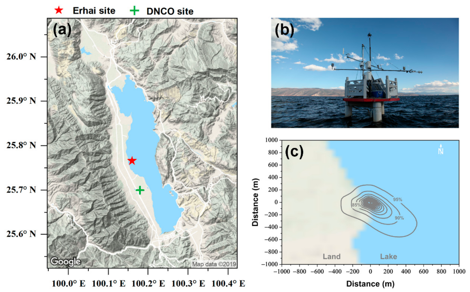
2.1. Observation Site and Instruments

Erhai Lake is located in the city of Dali, Yunnan Province in China. It is surrounded by the Cangshan Mountains to the west and the Yu’an Mountains to the east (Figure 1). The Lake covers an area of 252.2 km2, with a south-north length of about 42.6 km and an east-west length of about 3–9 km. The average and maximum depths are 10 m and 20.7 m, respectively. This region lies in a subtropical monsoon climate zone, which is characterized by a warm-wet season from May to October and a cold-dry season from November to April [35]. According to the local climatology record [36], the monthly mean air temperature ranges from 8.4 °C in December to 20.3 °C in June, and the annual mean precipitation is 1055 mm, with 85% of precipitation concentrated in the wet season. There are mainly 18 rivers and streams from the foothills of Cangshan mountain flowing into the lake, and exists only one natural outlet-Xi’er River in the south. The water level is controlled artificially due to the agricultural irrigation for cropland during dry season, and ranges from 1971.1 m to 1974.1 m [37]. The water body is ice-free all year round and well mixed without obvious thermal stratification [38].
The platform (25.46° N, 100.10° E) is established approximately 70 m away from the west bank of Erhai Lake (Figure 1). The height between the platform and the water surface ranged from 1.5 m to 3 m with the changing water level. The EC instruments were mounted at 2 m above the platform. The fluctuations of wind velocity components ( u , v and w ) and sonic temperature are captured by a three-dimensional sonic anemometer (CSAT3, Campbell Scientific, Logan, UT, USA). The water vapor and carbon dioxide density fluctuation are measured by an open-path infrared gas analyzer (IRGA, LI-7500, LI-COR, Lincoln, NE, USA). The data sampling frequency is 10 Hz. Sensors measured incoming and outgoing shortwave/longwave radiation (CNR1, Kipp and Zonen, Delft, The Netherlands) and active photosynthetic radiation (PAR, LI-190SB, Cambell Scientific, Logan, UT, USA) were mounted at 1.5 m above the platform. Air temperature and relative humidity are measured by HMP45C (Vaisala, Vantaa, Finland), and wind speed/direction was measured by 034B (Met One Instruments, Grants Pass, OR, USA) at 2.5 m above the platform. The water temperature profile at 0.05, 0.2, 0.5, 1, 2, 4, 6 and 8 m under the water surface are measured by water temperature sensors (CS616, Campbell Scientific, Logan, UT, USA). Measurement of basic meteorological variables and water temperature profile are taken every minute and recorded as 30-min averaged values. More information on the observation site and instruments is already documented in our previous study [39].

2.2. EC Data PostProcessing

The EC measurement dataset during the period from 2015 to 2018 was analyzed in this study. The raw 10 Hz, time-series data were processed into 30-min average values with the EddyPro software, Version 6.1 (LI-COR, Inc. 2015, Lincoln, NE, USA). The raw data point was considered as a spike when its magnitude exceeded the mean values 3.5 times the standard deviations within a certain moving time window and was further replaced through linear interpolation [40]. The double rotation method was adopted to align the x-axis wind component to the local streamline and turn the vertical and crosswind component into zero [41]. The block average based on the Reynolds decomposition rule was applied to remove a trend in the raw time series and obtain the fluctuations. Therefore, Latent and sensible heat fluxes were calculated from 30-min to mean covariances between the fluctuations of the scalars and the vertical wind speed component. Correction for density fluctuations was applied to latent heat and CO2 fluxes using the method developed by [42]. The data quality control was applied to EC 30-min fluxes using the 0-1-2 flag system [43], which the fluxes with flag = 0 have the best quality, with flag = 1 is suitable for general analysis, and with flag = 2 do not pass the steady-state test and the developed turbulent conditions test and needed to be abandoned. Moreover, the data points were also removed when active gain control (AGC) values larger than 40 indicated the low-quality data caused by precipitation, dust, or other contamination on the sensor optics. Because the EC observation site is located near the west side of the lake, the flux footprint area is calculated by the footprint model [44]. As shown in Figure 1c, direction 225–315° contains fluxes from the land surface is removed to eliminate the influence of the surrounding land area. After the data filtering as described above, the remaining 30-min data for sensible and latent heat fluxes are 69.8% and 74.3% in 2015, 67.1% and 70.8% in 2016, 69.7% and 72.0% in 2017, and 68.9% and 75.2% in 2018, respectively. To estimate the annual budgets of evaporation, an artificial neural network (ANN) method [38] is applied to fill the data gap in the daily timescale. The network was trained with four observed meteorological variables, including wind speed, air temperature, vapor pressure difference, and net radiation. The annual total evaporation losses are 1264.0 mm, 1214.6 mm, 1266.1 mm, and 1299.6 mm during 2015, 2016, 2017, and 2018, respectively.
To obtain the interannual variation of lake evaporation, a long term dataset (1981–2018) from measurements in the neighboring Dali National Climatic Observatory (DNCO, [36]) site and gridded China Meteorological Forcing Dataset (CMFD, [45,46]) are selected in this study. The DNCO site is about 15 km away from the Erhai Lake site (Figure 1a). The CMFD dataset was made through a fusion of remote sensing products, a reanalysis dataset and in situ observation data at the weather station, with a spatial resolution of 0.1° and temporal resolution of three hours. Variables of wind speed, air temperature, relative humidity and precipitation are obtained from the DNCO measurements dataset. Incoming solar radiation is obtained from the long-term CMFD dataset. Using the land-based forcing data will likely introduce errors in calculating lake evaporation. Corrections of input variables were made to reduce systematic errors by comparing the land-based data with in situ measurements of Erhai Lake.

2.3. Introduction of Evaporation Methods

Nine evaporation methods based on different physical constraints and data requirements were selected for the estimation of open-water evaporation and classified into three categories, including the combination methods, solar radiation-based methods and Dalton-based methods.

2.3.1. Combination Methods

The Bowen ratio energy budget (BREB) method was first introduced by [18] and was generally regarded as a standard method for estimating evaporation over water surfaces in the absence of in situ observation [1,25]. The formula of the BREB method is given as follows:
E = R n Δ Q ρ w λ 1 + β + T s c p w × D
β = c p P ( T s T a ) ε λ ( e s * e a )
e s * = 0.611 e x p 17.27 T s 237.3 + T s
e a * = 0.611 e x p 17.27 T a 237.3 + T a
e a = e a * R H 100
Δ Q = ρ w c p w Δ T w Δ t z d
where E is the estimated evaporation rate (mm d−1), R n is the net radiation (W m−2), Δ Q is the heat storage change in the water body (W m−2), ρ w is the water density (1000 kg m−3), λ is the latent heat of vaporization (2.45 × 10⁶ J kg−1), β is the Bowen ratio (dimensionless), T s is the water surface temperature (°C), T a is the air temperature (°C), P is the atmospheric pressure (kPa), ε is the ratio of molecular weight of the water to that of the dry air (0.622, dimensionless), e s * is the saturated vapor pressure at the water surface temperature (kPa), e a * is the saturated vapor pressure at the air temperature (kPa), e a is the vapor pressure at the air temperature (kPa), R H is the relative humidity (%), c p w is the specific heat of water at constant pressure (4192 J kg−1 °C), c p is the specific heat of air at constant pressure (1004 J kg−1 °C), D is the multipliers that convert the unit of evaporation into mm d−1 (86.4 × 10⁶), Δ T w Δ t is the mean water temperature change during the time interval Δ t (°C s−1), z d is the largest depth at the profile measurement (m).
The Penman (PM) method [20] combined the surface energy budget and aerodynamic components, which was developed to calculate the potential evaporation from an open water surface. The PM equation is expressed as:
E = Δ Δ + γ R n Δ Q λ ρ w + γ f u e a * e a × 10 Δ + γ λ ρ w × D
Δ = 4098 0.611 e x p 17.27 T a T a + 237.3 ( T a + 237.3 ) 2
γ = c p P ε λ
f u = 3.6 + 2.5 U
where Δ is the slope of saturated vapor pressure–air temperature curve (kPa °C−1), γ is the psychometric constant (kPa °C−1), f u is the wind function (W m−1 hPa−1), U is the wind speed at the measurement height (m s−1). The first term of the PM method is usually defined as equilibrium evaporation; the lower limit of evaporation when the air above the water surface is saturated. The second term of the PM method is generally called the aerodynamic component correlated to the drying power of the air.
The Priestley–Taylor (PT) method [47] was originally developed for estimating potential evaporation over open water surfaces and saturated land surfaces under advection–minimum conditions. The PT method is a simple expression of the PM equation, which introduced a constant to account for the aerodynamic component of the PM method. The PT formula is expressed as:
E = α Δ Δ + γ R n Δ Q λ ρ w × D
where α is the Priestley–Taylor empirical constant and taken as a constant of 1.26.
The DeBruin–Keijman (dBK) method [48] is derived from the PT equation and determined as:
E = Δ 0.85 Δ + 0.63 γ R n Δ Q λ ρ w × D
The following empirical relationship between β and γ / [49] is applied in the derivation of the dBK method:
β = 0.63 γ 0.15
The Brutsaert–Stricker (BS) method [50] also called the advection–aridity model, is based on the concept of a symmetric complementary relationship that depends on the feedback between actual evaporation ( E a ) and potential evaporation ( E p ),
E a = 2 E w E p
where E w is the wet environment evaporation and is often calculated by the PT method, E p is generally calculated by the PM method. E a is the evaporation defined by the BS method, and therefore the formula can be written as:
E = 2 α 1 Δ Δ + γ R n Δ Q λ ρ w γ f u e a * e a × 10 Δ + γ λ ρ w × D

2.3.2. Solar Radiation-Based Methods

Two different generalized forms of solar radiation-based methods, including the Jensen–Haise (JH) method [51] and Makkink (Mak) method [52], were evaluated in this study. The JH method was originally developed for the arid environment in the western United States and determined by the following expression:
E = 0.014 1.8 T a + 32 0.37 R s λ ρ w × D
where R s is the incoming solar radiation (W m−2).
The Mak method was first developed for estimating evapotranspiration for grasslands in The Netherlands and is currently applied to open water. The equation is described as follows:
E = 0.61 Δ Δ + γ R s λ ρ w × D 0.012

2.3.3. Dalton-Based Methods

The Dalton-based methods, consisting of mass transfer (MT) method [21,53] and Ryan–Harleman (RyH) method [54], estimated the evaporation through wind speed ( U ) and vapor pressure difference (VPD) between the lake surface and the atmosphere. A simple formula of the MT method is given as follows:
E = N U e s * e a × 1000
N = 0.00338 A s 0.05
where N is the mass transfer coefficient and parameterized as a function of lake surface area A s (acre) [21].
The RyH method considered the two main evaporation-driven processes: free convection caused by buoyancy and forced convection caused by wind. The formula of the RyH method is given as follows:
E = 2.7 ( T s T a ) 1 3 + 3.1 U λ ρ w e s * e a × 10 × D

2.4. Calibration of Evaporation Methods

Due to the difference in physical and climatic conditions, some parameters or empirical coefficients can be replaced or calibrated to achieve a relatively better agreement with observations. The details of the adjustments are summarized in Table 1. Since long term continuous observation of temperature profiles sometimes is absent because of the instrument failure, the determination of heat storage in the water body needs alternate expression related to meteorological factors. For the combination methods, the heat storage is determined using the measured water temperature profiles in the default condition (V0) and a hysteresis function of net radiation [55] in the calibrated condition (V1), respectively. The initial climate conditions assumed for the two solar radiation-based methods are totally different from the Erhai Lake, and therefore its empirical coefficients are calibrated site-specific through multiple regression against measured evaporation. The transfer coefficient N for the MT method, which reflects the efficiency of vertical transport of water vapor by turbulent eddies induced from wind shear, is calibrated by using the aerodynamic formula [22]. The empirical constants of the RyH method are also modified by forcing multiple regression against measured data under the condition V1.

2.5. Evaluation Criteria of Evaporation Methods

To evaluate the performance of evaporation methods from daily to monthly timescale, statistical measures including linear correlation coefficient (R), root mean square error (RMSE) and mean absolute error (MAE) between the observed and estimated evaporation were selected and calculated as follows:
R = i = 1 n O B S i O B S ¯ M O D i M O D ¯ i = 1 n O B S i O B S ¯ 2 i = 1 n M O D i M O D ¯ 2
RMSE = 1 n i = 1 n M O D i O B S i 2
MAE = 1 n i = 1 n M O D i O B S i
where n denotes the number of data points, O B S i and M O D i are the observed and modeled evaporation, respectively, O B S ¯ and M O D ¯ are mean values of the observed and modeled evaporation, respectively.

2.6. Assessment of Relative Contribution

In order to quantify the relative contribution of meteorological factors to the long-term trend of annual evaporation, the detrend method [56] and the sensitivity method [57] were used. In the detrend method, the relative contribution of a factor x i is determined by the following formula:
R C d e t r e n d x i = d E o r i g i n a l d t     d E d e t r e n d   x i d t j = 1 n t d E o r i g i n a l d t     d E d e t r e n d   x j d t × 100 %
where R C d e t r e n d x i is the relative contribution of factor x i to evaporation changes based on the detrend method, d E o r i g i n a l d t is the trend of lake evaporation calculated by using the original inputs, d E d e t r e n d   x i d t is the trend of lake evaporation calculated by using the linear detrend x i and original data for other variables, n t is the total number of affecting factors. In the sensitivity method, the relative contribution of a factor x i is determined by the following formula:
R C s e n s i t i v i t y x i = E o r i g i n a l x i   d x i d t j = 1 n t E o r i g i n a l x j   d x j d t × 100 %
where R C s e n s i t i v i t y x i is the relative contribution of factor x i to evaporation changes based on the sensitivity method, E o r i g i n a l x i is the partial derivatives of x i , d x i d t is the trend of x i during the long-term period.

3. Results and Discussions

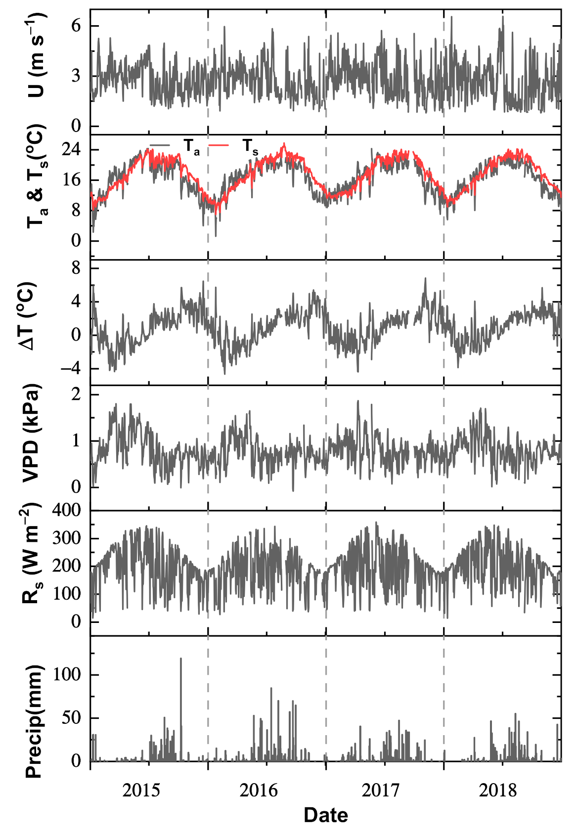
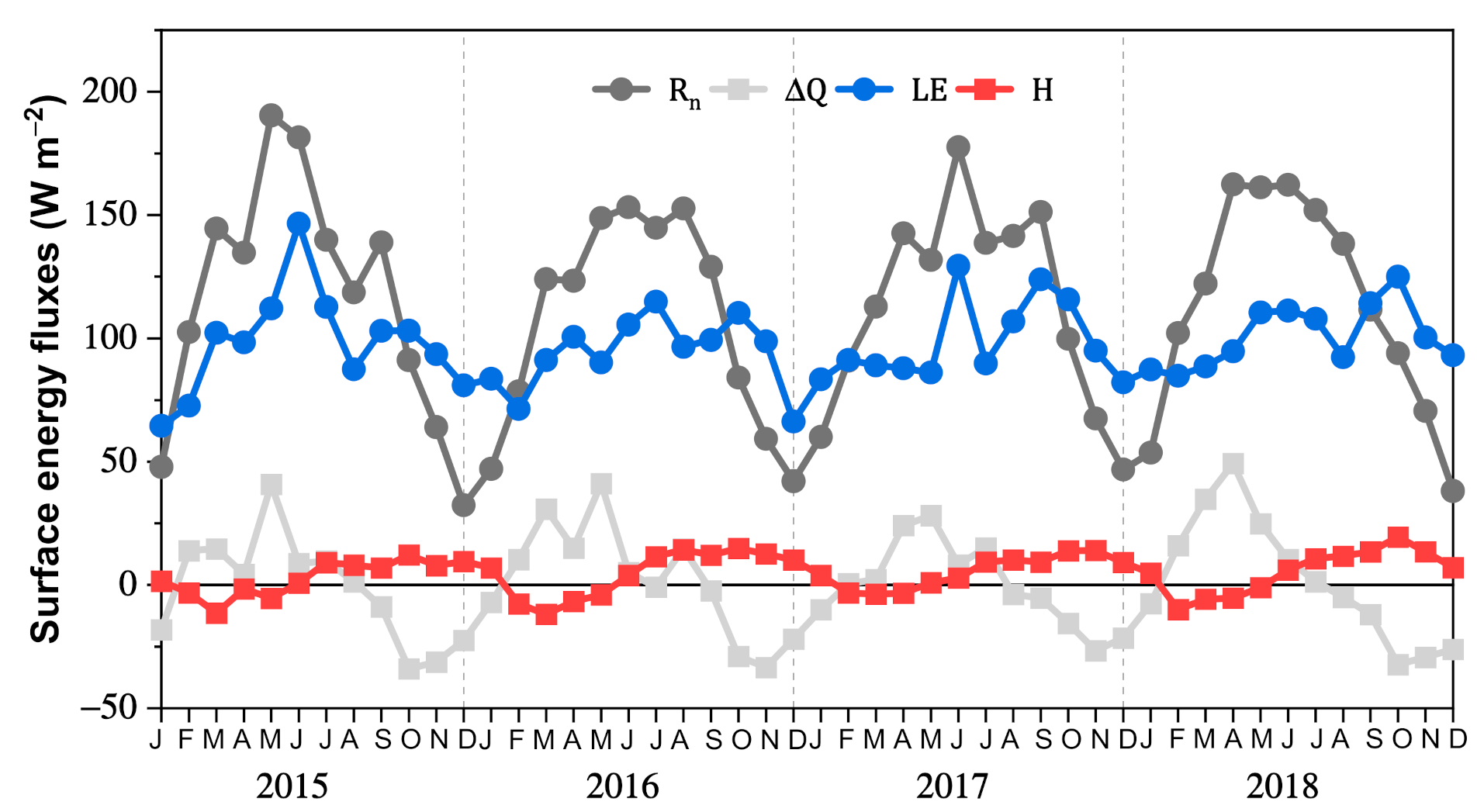
3.1. Meteorological Conditions and Surface Energy Budget

The general characteristic of meteorological conditions during 2015–2018 is shown in Figure 2. Daily average wind speed ( U ) ranged from 0.80 to 6.58 m s−1 during 4-year period. The annual mean values of U from 2015 to 2018 were 2.80 m s−1, 2.70 m s−1, 2.90 m s−1, and 2.69 m s−1, respectively. The annual mean U in each year was slightly higher than the long-term annual average of 2.50 m s−1 for the period 1981–2010 at the Dali National Climatic Observatory (DNCO). Air temperature ( T a ) and water surface temperature ( T s ) both showed clearly seasonal variation. Noted that T s is derived from the longwave radiation. Daily average T a ranged from 1.3 to 24.3 °C. The measured annual average values of T a from 2015 to 2018 were 1.41~1.64 °C warmer than the long-term climate average of 15.06 °C for the period 1981 to 2010. Daily average T s ranges from 7.0 °C to 25.8 °C during 2015–2018. The annual average T s during 2015–2018 ranged from 17.43 °C to 17.69 °C, which were slightly larger than the annual mean T a . The daily average temperature difference ( Δ T ) between the lake surface and the atmosphere was almost negative from February to June and was positive during other months in a year. Annual mean Δ T is always positive during 4-year period. The daily average vapor pressure difference (VPD) gradually increased with seasons but slightly dropped in summer due to a large amount of rainfall. The daily average incoming solar radiation ( R s ) generally peaked in mid-summer and reached its minimum in winter. Small daily mean values of R s were also observed in summer because of the influence of rainfall events. The precipitation was mainly concentrated on the monsoon season from May to October, accounted for 76% to 89% of the annual precipitation during 2015–2018. The annual total precipitation in 2016 (1153.6 mm) was larger than the long-term mean annual precipitation (1055 mm), while the annual precipitation in 2015 (1016.2 mm), 2017 (909.7 mm), and 2018 (1000.8 mm) were slightly lower than the long-term average.
The monthly mean value of surface energy budget components during 2015–2018 is shown in Figure 3. Net radiation ( R n ) displayed a strong seasonal variation, where maximum R n occurred in May of 2015 and June of 2016–2018, and minimums occurred in December with monthly average values lower than 50 W m−2. Seasonal variation of latent heat flux ( L E ) was similar to that of R n . Maximum monthly average L E was not consistent among four years and occurred in June of 2015 and 2017, July of 2016, and October of 2018, respectively. The maximum L E was about one month to three months lag behind the maximum R n over Erhai Lake. For large and deep lakes with the high heat capacity of lake water, a two to five months delay between maximum L E and R n was observed [17,58,59,60]. The seasonal variation of the heat storage change ( Δ Q ) can be divided into storaging period ( Δ Q > 0) and releasing period ( Δ Q < 0). The heat was absorbed into the water body during spring to summer and used to warm the lake water. The peak value of heat absorption was observed in May. A slight fluctuation of heat absorption occurred during summer due to a large amount of rainfall. The heat released into the atmosphere since September. The maximum heat release usually occurred from October to November. The seasonal variation of Δ Q has a significant influence on the estimation of seasonal lake evaporation by weakening evaporation during spring and summer and enhancing it largely during the autumn and winter [61].
The sensible heat flux ( H ) was relatively small when compared with L E , with monthly average values ranged from −11.9 W m−2 to 19.5 W m−2. Monthly mean H was usually remained negative from February to June when T a is greater than T s and became positive afterward when T a is smaller than T s . Based on the surface energy partitioning, most of the R n absorbed by the water body was consumed for lake evaporation with annual mean L E / R n ranged from 0.85 to 0.88 during 2015–2018. Monthly L E / R n exceeded 1 during September (only for 2018)/October to January, indicated the energy stored in the water body served as an additional energy source of evaporation during these periods. A similar result was also found in Ross Barnett Reservoir under humid and subtropical climate, with an annual average L E / R n of 0.81 and monthly average L E / R n > 1 during September to January [62]. For a hypersaline terminal lake under an arid environment, L E accounted for a lower portion of R n with an average value of 65% over four seasons [34]. The energy balance closure (EBC) is quantified by the ratio of the turbulent flux ( L E + H ) to the available energy ( R n Δ Q ). Annual mean energy EBC ranged from 0.86 to 0.97 during 2015–2018 and was comparable to values obtained from other lakes [15,31,62] and terrestrial sites [63].

3.2. Evaluation of Evaporation Methods at Different Timescales

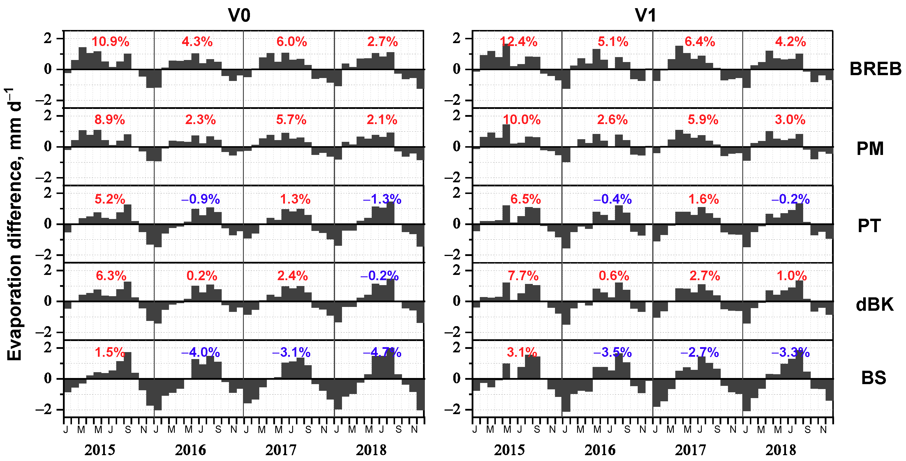
3.2.1. Evaluation of Combination Methods

The performances of five combination methods were improved as the timescale is extended from daily to monthly. Under the default condition V0, the mean correlation coefficient (R) of the five methods increased from 0.53 for daily to 0.85 for monthly timescale, the RMSE decreased from 1.85 to 0.83, and the MAE reduced from 1.30 to 0.67, respectively (Table 2, V0). Under the calibrated Condition V1, the heat storage change Δ Q is considered as a hysteresis function of R n . The estimate of evaporation using hysteresis Δ Q was also comparable to the default condition using measured Δ Q as input. The coefficient of determination R2 between measured and modeled Δ Q is 0.84 at monthly timescales during 2015–2018, which is identical to the average results of 22 lakes [55]. Using hysteresis relation is able to provide reasonable Δ Q estimates when measurements of water temperature profiles are not available, and produce good estimates of monthly evaporation for the combination methods. Reasonable evaporation estimates can also be achieved by taking heat storage as a simple linear function of R n in Poyang lake [64] with a mean depth of 8 m comparable to the mean depth of Erhai Lake (10 m).
The difference in monthly average evaporation between five combination methods and EC observations showed small seasonal bias under the default and calibrated conditions. The combination methods overestimated evaporation during spring and summer and underestimated it during late autumn to winter (Figure 4). Variation of seasonal bias was almost consistent among the five combination methods. Under the default condition V0, the departure was within the range of −1.5 mm d−1 to 1.5 mm d−1, except for the BS method with bias beyond this range. Calibrated condition V1 showed similar seasonal bias related to default condition V0. More positive bias during April (2017 and 2018) and May (2015 and 2016) and less negative bias during December were found in V1 (Figure 4, V1). Such seasonal bias of combination methods has also been found in other lakes [25,30,34,65]. The combination methods are based on the assumption of closed surface energy balance. However, the turbulent fluxes measured by the EC system are generally underestimated, and therefore, the surface energy balance is not always closed [66], eventually leading to seasonal deviation of combination methods.
On an annual basis, the difference in annual total evaporation loss displayed large variability, i.e., the BREB and PM method both overestimated the annual evaporation under default and calibrated condition during 2015–2018, while the BS method showed a slight overestimation in 2015 and underestimation during 2016–2018 (Figure 4). Compared to other combination methods, the larger underestimate during winter of the BS method balanced the positive bias and therefore resulted in small overestimation in 2015 and underestimation during 2016–2018. The PT and dBK methods showed relatively small annual bias during 4-year period. Annual evaporation loss estimated by the combination methods neglecting Δ Q did not change significantly in comparison with the inclusion of Δ Q (not shown), because the storage and release of energy from the lake were almost balanced with an annual mean of −1.78 to 2.04 W m−2 during 2015–2018. The heat storage can be roughly neglected on longer timescales.
Among all the combination methods, the PM method has the best performance with large R and small RMSE and MAE under the range of daily to monthly timescales, followed by the PT, dBK, BREB, and BS method. Good performance of the PM method is also found in other lakes, e.g., a large deep lake in Egypt [29], the Dead sea in an arid environment [34], and the Laja Lake in the middle of the Andes mountain range [67]. More favorable results from the PT than the dBK method coincided with the analysis in a small highland lake, which pointed out the PT method is more suitable for estimating evaporation over high altitude lakes than the dBK method developed from the sea-level environment [32]. The P-T coefficient taken as a constant of 1.26 without consideration its seasonal variability (larger than 1.26 in winter and smaller than 1.26 in summer, not shown) might introduce uncertainties and cause larger RMSE and MAE of the PT method in comparison with the PM method. However, in Poyang lake, a large shallow subtropical lake in China, no obvious seasonal trend in α was observed [68], and the PT method performed slightly better than the PM method [64]. The BS method displayed the largest bias for lake evaporation estimation among the combination methods from daily to monthly timescales, where its MAE value was almost twice as much as the value from the PM method.

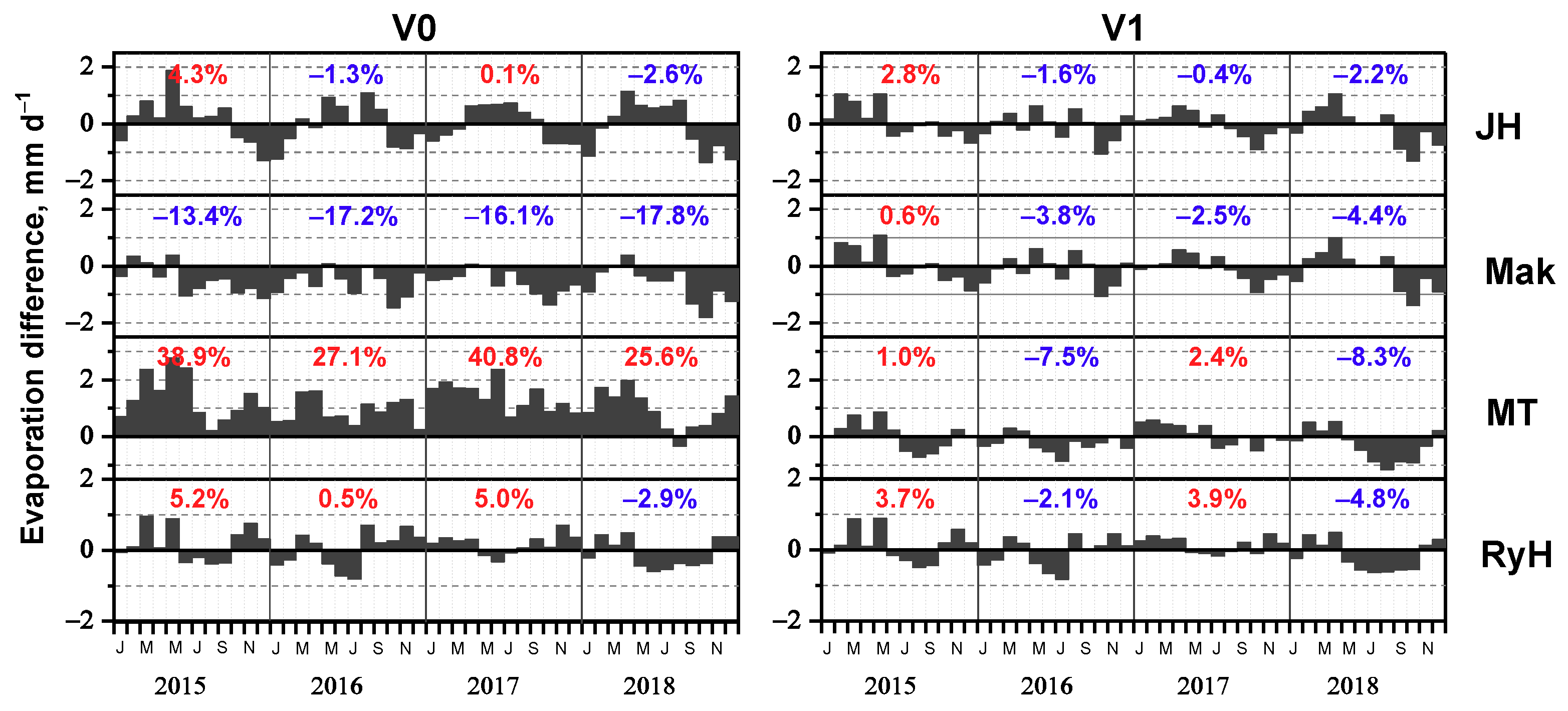
3.2.2. Evaluation of Solar Radiation-Based Methods

The performances of the solar radiation-based methods were similar to the combination methods. The radiation-based methods yielded poor estimates at short timescales (daily to weekly) and relatively good estimates at monthly timescale. Under the condition V0, the default version of two radiation-based methods compared less favorably with most of the combination methods, except for the BS method. The difference in monthly average evaporation between the default JH method and EC observations also had a seasonal cycle, in which lake evaporation was generally overestimated during spring and summer and was underestimated during late autumn and winter, resulting in an annual bias of −2.6% to 4.3% during 2015–2018 (Figure 5, V0). The default Mak method underestimated the monthly average evaporation almost all year, leading to a large negative annual bias of −13.4% to −17.8% during 2015–2018 (Figure 5, V0). Under the calibrated condition V1, the simulation bias of the default radiation-based methods was reduced after calibration with smaller RMSE and MAE, while the correlation between observation and modified JH method declined slightly compared to the default JH method (Table 2, V1). The large positive bias of the default JH method in summer was reduced or became negative after calibration (Figure 5, V1). The difference in annual bias caused by the JH method before and after calibration was not significant. The modified Mak method reduced the large negative deviation of default condition and overestimated evaporation during spring, consequently resulting in less negative annual bias ranged from −4.4% to 0.65% during 2015–2018 (Figure 5, V1). For the sake of simplicity and accuracy, the modified solar radiation-based methods have an advantage over the combination methods and were applied in estimating the long-term lake evaporation [32,69].

3.2.3. Evaluation of Dalton-based Methods

In contrast to the two former methods based on the surface energy budget and solar radiation, the Dalton-based methods had a larger correlation with observations at short timescales (daily to weekly) and relatively poor correlation at a monthly timescale. Under the default condition V0, the RyH method had much better performance than the MT method in terms of smaller RMSE and MAE values among the entire range of timescales (Table 2, V0). With the transfer coefficient N parameterized as a function of the lake surface area [21], the default MT method strongly overestimated the monthly average evaporation during all the year except for August 2018, thus leading to overestimation of the annual total evaporation by 25.7% to 40.6% during period 2015–2018 (Figure 5, V0). A similar result was also found in Lake Taihu [31] that the MT method caused an overestimation of annual evaporation up to 87%. For the default RyH method, the monthly departure of evaporation was within the scope of −1 to 1 mm d−1. The underestimation generally occurred during summer to early autumn. The annual bias was relatively small and varied from −2.9% to 5.2% during 4-year period (Figure 5, V0). Under the calibrated condition V1, two modified Dalton-based methods both reduced the bias in terms of smaller RMSE and MAE values from daily to monthly scales (Table 2, V1) compared to the default condition. Continuous strong overestimation of monthly average evaporation of default MT method was reduced substantially after using the aerodynamic formula of mass transfer coefficient N , and generally shifted into negative bias during the second half the year, resulting in a small positive annual bias in 2015 and 2017, and negative annual bias in 2016 and 2018 (Figure 5, V1). The difference in an annual bias of the RyH method was not significant before and after calibration, indicated the RyH method without site-specific calibration performed well over Erhai Lake. The good behavior of the default RyH method is also found in the study of a variety of lakes and ponds in Minnesota [70] and small mountain lakes in southern Wyoming, USA [71] because of the large variability in wind speed and relative humidity.

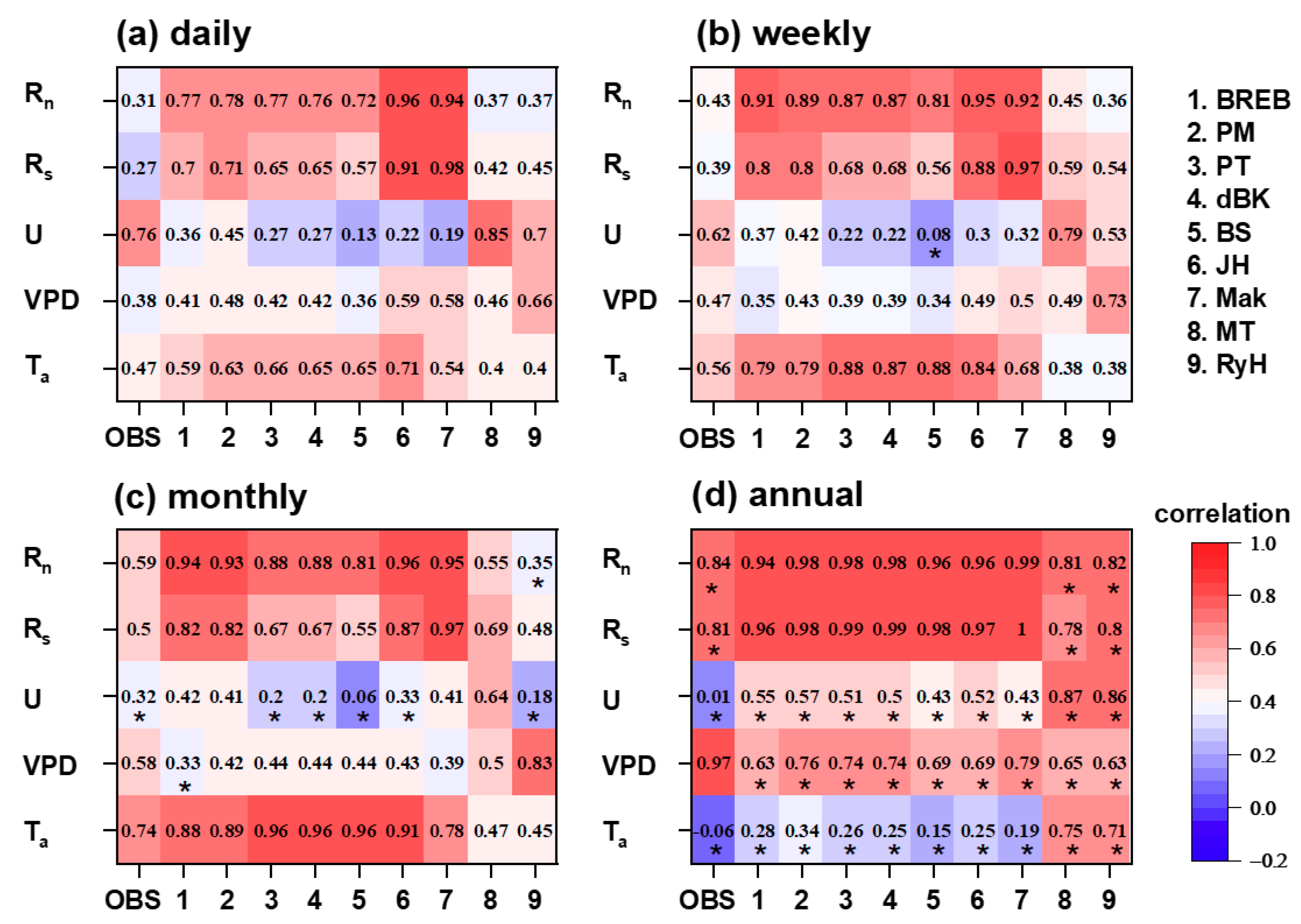
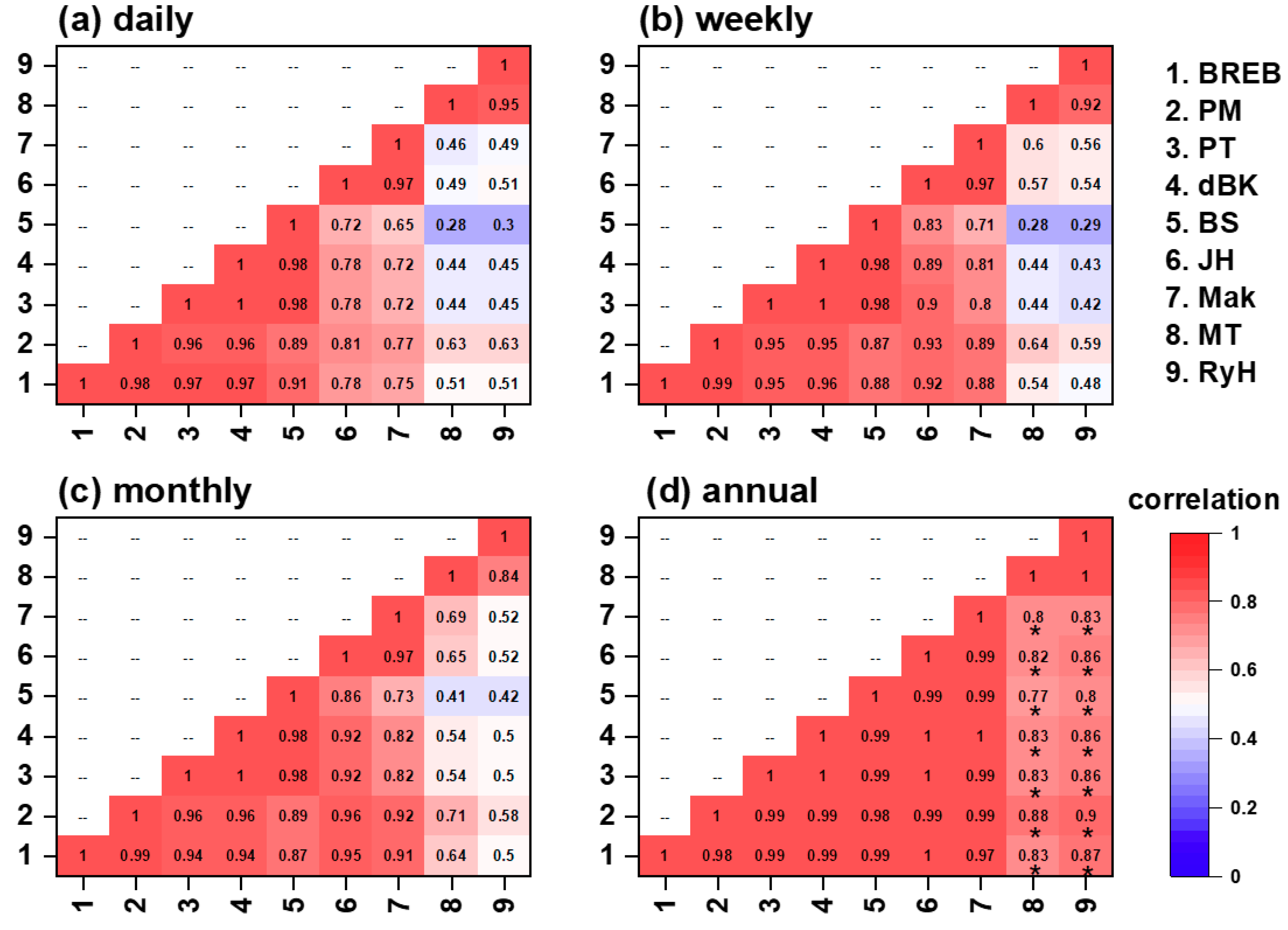
3.3. Inter-Comparisons between Evaporation Methods at Different Timescales

Nine evaporation methods are related to different main drivers of lake evaporation. The correlation between meteorological variables and lake evaporation obtained from observations and default evaporation methods across daily to yearly timescales during 2015–2018 is shown in Figure 6. On the basis of the measurement results, lake evaporation had the largest correlation with U from daily to weekly timescale, and the relationship gradually decreased as the time interval is extended, which correlation dropped from 0.76 on a daily scale to 0.01 on a yearly timescale. Lake evaporation had a greater correlation with T a and R n on a monthly timescale. On an annual timescale, evaporation was highly correlated to VPD and radiation ( R n and R s ) with a correlation higher than 0.8, while it had a negligible relationship with U and T a . Apparently, VPD, R n , and R s both had an increasing correlation with lake evaporation as the timescale is extended from daily to annual.
The combination and solar radiation-based methods failed at short timescales (daily to weekly), due to the mismatched controlling factors as lake evaporation was highly correlated with U while these methods were controlled by T a and radiation ( R n and R s ), and showed relative good performances at monthly timescale due to the consistency of large relationship with T a and radiation ( R n and R s ). The Dalton-based methods showed large correlations with U and VPD, make it possible to yield good estimates of evaporation from daily and weekly timescale, while produced less satisfactory results at monthly timescale because lake evaporation is largely correlated to T a and radiation. Due to the difference in weather and climatic conditions, lake evaporation dynamics are driven by different atmospheric forcing and processes, which will influence the suitability of evaporation methods among lakes. For instance, the good performance of calibrated Dalton-based methods during a shorter timescale over Erhai Lake is different from the results from lake Okeechobee in subtropical South Florida [72], because lake Okeechobee experienced a large amount of rainfall and small VPD condition, lake evaporation is mainly governed by solar radiation. Therefore, the Dalton-based methods driven by U and VPD is not suitable, and the solar radiation-based methods can provide more realistic estimates of evaporation. The solar radiation-based methods also have an advantage over the Dalton-based methods in estimating evaporation from lakes and reservoirs in a semi-arid environment [30].
The combination methods agreed well with the solar radiation-based methods across the entire range of timescale as they have similar controlling factors- T a and radiation ( R n and R s ) (Figure 7). These two methods showed obvious disagreement with the Dalton-based methods at shorter timescales because the latter is mainly driven by U and VPD, indicated the importance of choosing the appropriate method for lake evaporation estimation at a smaller timescale. The correlations between the methods increased with the extended timescale, indicated that the deviation of methods based on different physical parameterization would be reduced on a longer timescale. Despite the more consistency at the annual timescale, large differences could still occur between these methods.

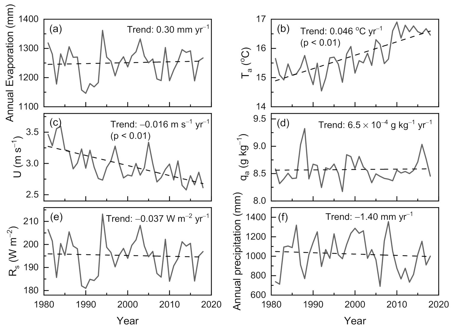
3.4. Estimation of Long-Term Lake Evaporation

To investigate the interannual variation of lake evaporation during the past decades (1981–2018), the calibrated JH method was forced with historical measurements dataset from the DNCO station and the CMFD dataset. The calibrated JH method had a relatively small annual bias varied from −2.6% to 2.8% during 2015–2018 (Figure 4, V1), and only required T a and R s as input, which both easily obtained, therefore made it become a practical and reliable option for estimating the long-term trend of evaporation.
The estimated annual evaporation displayed an insignificant increasing trend of 0.30 mm year−1 during 1981–2018 and ranged from 1146.2 mm to 1362.0 mm with a mean value of 1249.0 mm (Figure 8a). The low annual evaporation in the early 1990s resulted from the small incoming solar radiation. The increasing trend of lake evaporation has also been reported in lakes with different climate background, including a small highland lake in the Tibetan Plateau [32], Lake Taihu in a subtropical region of China [73], Lake IJssel in the Netherlands [69] and a small reservoir in the Brazilian savannah [74]. The long-term trend of evaporation of Erhai Lake calculated by the modified JH method is opposite to the results obtained from evaporation pan E601 situated in the surrounding land site [75], in which pan evaporation showed an obvious decreasing trend since the 1980s with rising temperature. This inverse trend is known as the “evaporation paradox”, which is in agreement with the results from reservoirs in the contiguous United States [76]. This discrepancy is likely attributed to different environmental and meteorological conditions and the limited measured area of the evaporation pan. During period 1981–2018, T a increased significantly with a trend of 0.046 °C year−1, while U declined significantly at a rate of −0.016 m s−1 year−1, R s and annual total precipitation both decreased slightly at rates of −0.037 W m−2 year−1 and −1.4 mm year−1, and specific humidity q a changed insignificantly (Figure 8). The increasing lake evaporation accompanied by decreasing precipitation is likely to reduce the water resources of Erhai Lake, which is supported by the decreasing trend of water resources observed in this basin [77] and in the mainland of China [78]. The climate over Erhai Lake basin was mainly cold and wet in the 1960s and 1970s, but getting warm after into 1980s and warmer and dry into the 21st century [77]. This changing climatic condition may cause an increase in lake evaporation since the 1980s despite the incoming solar radiation decreased during this period.
The relative contributions of T a and R s were quantified by the detrend method and sensitivity method to find out what caused the evaporation trend during the past decades, as shown in Figure 9. A large difference occurred between the original evaporation and the recalculated evaporation under the detrended T a condition. The increasing trend (0.30 mm year−1) of evaporation based on the original inputs was largely reduced to −0.24 mm year−1 when using the detrended T a and original R s as input (Figure 9c). Under the detrended R s condition, the trend of original annual evaporation was slightly increased to 0.54 mm year−1 (Figure 9c). Based on the detrend method, the increasing T a contributed to 69.2% of evaporation variation, while the decreasing R s resulted in −30.8% of evaporation change (Figure 9f). Relative contributions of these two factors based on the sensitivity method were consistent with the results of the detrend method. The change in T a contributed 69.5% to evaporation variation (Figure 9f). Therefore, the rising T a contributed to the increasing trend of evaporation during 1981–2018, indicating the impact of changing climate on the hydrological cycle over Erhai Lake. Because the variation of R s was relatively small and insignificant during 1981–2018, its contribution to the long-term trend of evaporation was not the largest, although the magnitude of annual lake evaporation changed largely to the disturbance of R s . It has been reported that annual evaporation for lakes in low-altitude areas is projected to increase about 200 mm by 2091–2100 in comparison with 2006–2015, in spite of little changes in incoming solar radiation [8]. According to a study about the characteristics of climate change around the Erhai Lake area, the annual average air temperature will keep a warming trend in the future [79], which may continuously accelerate the evaporation of the lake and, in turn, alter the local water balance and energy budget allocation.

4. Conclusions

This study is aimed to evaluate the nine evaporation methods at different timescales on the basis of the comprehensive measurements conducted by an EC system over the Erhai Lake and revealed the long-term trend of evaporation. The accuracy of methods varied with timescales resulted from the (dis)agreement between its parameterization scheme and the drivers of lake evaporation. Under the default condition, the Dalton-based RyH method is the most accurate method at short timescales (daily to weekly), while the MT method resulted in a large overestimation of lake evaporation. On a monthly scale, the variation of lake evaporation is better described by the combination and solar radiation-based methods since evaporation is mainly correlated to air temperature and radiation ( R n and R s ). Under the calibrated condition, the combination methods using the hysteresis heat storage produced comparable results to the default condition using measured heat storage as input, indicated the hysteresis model could be considered as a good alternative for estimating heat storage without the measurement of water temperature profiles. The JH and RyH method improved slightly after optimization. The large negative bias of the default Mak method and positive bias of the default MT method were substantially reduced after optimization. The calibrated JH method had a relatively small annual bias, and a simple data requirement was applied in the estimates of long-term evaporation. The annual total evaporation showed an insignificant increasing trend of 0.30 mm year−1 during 1981–2018, with a minimum occurred in the early 1990s. Relative contributions of meteorological factors were quantified by the detrend method and sensitivity method. Rising air temperature contributed to the increasing trend of evaporation by 69.2% and 69.5% based on the detrend method and sensitivity method, respectively. This result indicated the amplified impact of a warming climate on the water cycle over the Erhai Lake basin, which will help to better understand the response of the lake system to climate change. In this study, we only concentrated on the estimate of historical evaporation. The extent of lake evaporation over Erhai Lake in the future and its variability are underexplored and needed to discuss further.

Author Contributions

H.L. designed the measurement platform over Erhai Lake. Y.L. carried out the in situ measurement. Q.D., L.X., and X.M. analyzed the data. X.M. wrote the original draft and all the authors contributed to the revision of the manuscript. All authors have read and agreed to the published version of the manuscript.

Funding

This study was supported by the National Key Research and Development Program of China (No. 2017YFC1502101) and the National Natural Science Foundation of China (No. 41775018 and No. 41805010).

Acknowledgments

We thank the staffs in Yunnan Provincial Institute of Meteorology and Dali National Climatic Observatory for helping the maintenance of the measurement site and instruments, and the National Tibetan Plateau Data Center for providing the long-term China meteorological forcing dataset.

Conflicts of Interest

The authors declare no conflict of interest.

References

  1. Gianniou, S.K.; Antonopoulos, V.Z. Evaporation and energy budget in Lake Vegoritis, Greece. J. Hydrol. 2007, 345, 212–223. [Google Scholar] [CrossRef]
  2. Oki, T. Global Hydrological Cycles and World Water Resources. Science 2006, 313, 1068–1072. [Google Scholar] [CrossRef] [PubMed] [Green Version]
  3. Koutsoyiannis, D. Revisiting the global hydrological cycle: Is it intensifying? Hydrol. Earth Syst. Sci. 2020, 24, 3899–3932. [Google Scholar] [CrossRef]
  4. O’Reilly, C.M.; Sharma, S.; Gray, D.K.; Hampton, S.E.; Read, J.S.; Rowley, R.J.; Schneider, P.; Lenters, J.D.; McIntyre, P.B.; Kraemer, B.M.; et al. Rapid and highly variable warming of lake surface waters around the globe. Geophys. Res. Lett. 2015, 42, 10773. [Google Scholar] [CrossRef] [Green Version]
  5. Yang, K.; Yu, Z.; Luo, Y.; Zhou, X.; Shang, C. Spatial-Temporal Variation of Lake Surface Water Temperature and Its Driving Factors in Yunnan-Guizhou Plateau. Water Resour. Res. 2019, 55, 4688–4703. [Google Scholar] [CrossRef]
  6. Sharma, S.; Blagrave, K.; Magnuson, J.J.; O’Reilly, C.M.; Oliver, S.; Batt, R.D.; Magee, M.R.; Straile, D.; Weyhenmeyer, G.A.; Winslow, L.A.; et al. Widespread loss of lake ice around the Northern Hemisphere in a warming world. Nat. Clim. Chang. 2019, 9, 227–231. [Google Scholar] [CrossRef]
  7. Woolway, R.I.; Kraemer, B.; Lenters, J.D.; Merchant, C.J.; O’Reilly, C.M.; Sharma, S. Global lake responses to climate change. Nat. Rev. Earth Environ. 2020, 1, 388–403. [Google Scholar] [CrossRef]
  8. Wang, W.; Lee, X.; Xiao, W.; Liu, S.; Schultz, N.M.; Wang, Y.; Zhang, M.; Zhao, L. Global lake evaporation accelerated by changes in surface energy allocation in a warmer climate. Nat. Geosci. 2018, 11, 410–414. [Google Scholar] [CrossRef]
  9. Long, Z.; Perrie, W.; Gyakum, J.; Caya, D.; Laprise, R. Northern Lake Impacts on Local Seasonal Climate. J. Hydrometeorol. 2007, 8, 881–896. [Google Scholar] [CrossRef] [Green Version]
  10. Friedrich, K.; Grossman, R.L.; Huntington, J.; Blanken, P.D.; Lenters, J.D.; Holman, K.D.; Gochis, D.; Livneh, B.; Prairie, J.; Skeie, E.; et al. Reservoir Evaporation in the Western United States: Current Science, Challenges, and Future Needs. Bull. Am. Meteorol. Soc. 2018, 99, 167–187. [Google Scholar] [CrossRef]
  11. Xiao, K.; Griffis, T.J.; Baker, J.M.; Bolstad, P.V.; Erickson, M.D.; Lee, X.; Wood, J.D.; Hu, C.; Nieber, J.L. Evaporation from a temperate closed-basin lake and its impact on present, past, and future water level. J. Hydrol. 2018, 561, 59–75. [Google Scholar] [CrossRef]
  12. McMahon, T.A.; Peel, M.C.; Lowe, L.; Srikanthan, R.; McVicar, T.R. Estimating actual, potential, reference crop and pan evaporation using standard meteorological data: A pragmatic synthesis. Hydrol. Earth Syst. Sci. 2013, 17, 1331–1363. [Google Scholar] [CrossRef] [Green Version]
  13. Sene, K.; Gash, J.; McNeil, D. Evaporation from a tropical lake: Comparison of theory with direct measurements. J. Hydrol. 1991, 127, 193–217. [Google Scholar] [CrossRef]
  14. Liu, H.; Zhang, Y.; Liu, S.; Jiang, H.; Sheng, L.; Williams, Q.L. Eddy covariance measurements of surface energy budget and evaporation in a cool season over southern open water in Mississippi. J. Geophys. Res. Atmos. 2009, 114. [Google Scholar] [CrossRef]
  15. Nordbo, A.; Launiainen, S.; Mammarella, I.; Leppäranta, M.; Huotari, J.; Ojala, A.; Vesala, T. Long-term energy flux measurements and energy balance over a small boreal lake using eddy covariance technique. J. Geophys. Res. Atmos. 2011, 116. [Google Scholar] [CrossRef]
  16. Shao, C.; Chen, J.; Stepien, C.A.; Chu, H.; Ouyang, Z.; Bridgeman, T.B.; Czajkowski, K.P.; Becker, R.H.; John, R. Diurnal to annual changes in latent, sensible heat, and CO2 fluxes over a Laurentian Great Lake: A case study in Western Lake Erie. J. Geophys. Res. Biogeosciences 2015, 120, 1587–1604. [Google Scholar] [CrossRef]
  17. Philippe, C.; Ma, Y.-J.; Huang, Y.-M.; Hu, X.; Wu, X.-C.; Wang, P.; Li, G.-Y.; Zhang, S.-Y.; Wu, H.-W.; Jiang, Z.-Y.; et al. Evaporation and surface energy budget over the largest high-altitude saline lake on the Qinghai-Tibet Plateau. J. Geophys. Res. Atmos. 2016, 121, 10470. [Google Scholar] [CrossRef]
  18. Bowen, I.S. The Ratio of Heat Losses by Conduction and by Evaporation from any Water Surface. Phys. Rev. 1926, 27, 779–787. [Google Scholar] [CrossRef] [Green Version]
  19. Lenters, J.D.; Kratz, T.K.; Bowser, C.J. Effects of climate variability on lake evaporation: Results from a long-term energy budget study of Sparkling Lake, northern Wisconsin (USA). J. Hydrol. 2005, 308, 168–195. [Google Scholar] [CrossRef]
  20. Penman, H.L. Natural evaporation from open water, bare soil and grass. In Proceedings of the Royal Society of London. Series A, Containing Papers of a Mathematical and Physical Character; The Royal Society: London, UK, 1948; Volume 193, pp. 120–145. [Google Scholar]
  21. Harbeck, G.E. A Practical Field Technique for Measuring Reservoir Evaporation Utilizing Mass-Transfer Theory; U.S. Government Publishing Office: Washington, DC, USA, 1962; pp. 101–105.
  22. Brutsaert, W. Evaporation into the Atmosphere: Theory, History, and Application, 1st ed.; Kluwer Academic: Dordrecht, The Netherlands, 1982. [Google Scholar]
  23. Xu, C.Y.; Singh, V.P. Evaluation and generalization of radiation-based methods for calculating evaporation. Hydrol. Process. 2000, 14, 339–349. [Google Scholar] [CrossRef]
  24. Xu, C.-Y.; Singh, V.P. Evaluation and generalization of temperature-based methods for calculating evaporation. Hydrol. Process. 2001, 15, 305–319. [Google Scholar] [CrossRef] [Green Version]
  25. Rosenberry, D.O.; Winter, T.C.; Buso, D.; Likens, G.E. Comparison of 15 evaporation methods applied to a small mountain lake in the northeastern USA. J. Hydrol. 2007, 340, 149–166. [Google Scholar] [CrossRef]
  26. Finch, J.; Calver, A. Methods for the Quantification of Evaporation from Lakes; World Meteorological Organization’s Commission for Hydrology: Oxfordshire, UK, 2008. [Google Scholar]
  27. Duan, Z.; Bastiaanssen, W.G.M. Evaluation of three energy balance-based evaporation models for estimating monthly evaporation for five lakes using derived heat storage changes from a hysteresis model. Environ. Res. Lett. 2017, 12, 024005. [Google Scholar] [CrossRef] [Green Version]
  28. Singh, V.P.; Xu, C.Y. Evaluation and generalization of 13 mass-transfer equations for determining free water evaporation. Hydrol. Process. 1997, 11, 311–323. [Google Scholar] [CrossRef]
  29. Elsawwaf, M.; Willems, P.; Pagano, A.; Berlamont, J. Evaporation estimates from Nasser Lake, Egypt, based on three floating station data and Bowen ratio energy budget. Theor. Appl. Clim. 2009, 100, 439–465. [Google Scholar] [CrossRef] [Green Version]
  30. Majidi, M.; Alizadeh, A.; Farid, A.; Vazifedoust, M. Estimating Evaporation from Lakes and Reservoirs under Limited Data Condition in a Semi-Arid Region. Water Resour. Manag. 2015, 29, 3711–3733. [Google Scholar] [CrossRef]
  31. Wang, W.; Xiao, W.; Cao, C.; Gao, Z.; Hu, Z.; Liu, S.; Shen, S.; Wang, L.; Xiao, Q.; Xu, J.; et al. Temporal and spatial variations in radiation and energy balance across a large freshwater lake in China. J. Hydrol. 2014, 511, 811–824. [Google Scholar] [CrossRef]
  32. Wang, B.; Ma, Y.; Ma, W.; Su, B.; Dong, X. Evaluation of ten methods for estimating evaporation in a small high-elevation lake on the Tibetan Plateau. Theor. Appl. Clim. 2018, 136, 1033–1045. [Google Scholar] [CrossRef]
  33. McGloin, R.; McGowan, H.; McJannet, D.; Burn, S. Modelling sub-daily latent heat fluxes from a small reservoir. J. Hydrol. 2014, 519, 2301–2311. [Google Scholar] [CrossRef] [Green Version]
  34. Metzger, J.; Nied, M.; Corsmeier, U.; Kleffmann, J.; Kottmeier, C. Dead Sea evaporation by eddy covariance measurements vs. aerodynamic, energy budget, Priestley–Taylor, and Penman estimates. Hydrol. Earth Syst. Sci. 2018, 22, 1135–1155. [Google Scholar] [CrossRef] [Green Version]
  35. Du, Q.; Liu, H.; Xu, L.; Liu, Y.; Wang, L. The monsoon effect on energy and carbon exchange processes over a highland lake in the southwest of China. Atmos. Chem. Phys. 2018, 18, 15087–15104. [Google Scholar] [CrossRef] [Green Version]
  36. Xu, A.; Li, J. An Overview of the Integrated Meteorological Observations in Complex Terrain Region at Dali National Climate Observatory, China. Atmosphere 2020, 11, 279. [Google Scholar] [CrossRef] [Green Version]
  37. Du, Q.; Liu, H.; Liu, Y.; Wang, L.; Xu, L.J.; Sun, J.H.; Xu, A.L. Factors controlling evaporation and the CO2 flux over an open water lake in southwest of China on multiple temporal scales. Int. J. Clim. 2018, 38, 4723–4739. [Google Scholar] [CrossRef]
  38. Feng, J.W.; Liu, H.; Sun, J.H.; Wang, L. The surface energy budget and interannual variation of the annual total evaporation over a highland lake in Southwest China. Theor. Appl. Clim. 2015, 126, 303–312. [Google Scholar] [CrossRef]
  39. Liu, H.; Feng, J.; Sun, J.; Wang, L.; Xu, A. Eddy covariance measurements of water vapor and CO2 fluxes above the Erhai Lake. Sci. China Earth Sci. 2014, 58, 317–328. [Google Scholar] [CrossRef]
  40. Vickers, D.; Mahrt, L. Quality control and flux sampling problems for tower and aircraft data. J. Atmos. Ocean Technol. 1997, 14, 512–526. [Google Scholar] [CrossRef]
  41. Kaimal, J.C.; Finnigan, J.J. Atmospheric Boundary Layer Flows: Their Structure and Measurement, 1st ed.; Oxford University Press: Oxford, UK, 1994; p. 289. [Google Scholar]
  42. Webb, E.K.; Pearman, G.I.; Leuning, R. Correction of Flux Measurements for Density Effects Due to Heat and Water-Vapor Transfer. Q. J. Roy. Meteor. Soc. 1980, 106, 85–100. [Google Scholar] [CrossRef]
  43. Mauder, M.; Foken, T. Documentation and instruction manual of the eddy-covariance software package324 TK3. Abt. Mikrometeorol. 2004, 46. Available online: https://core.ac.uk/download/pdf/33806389.pdf (accessed on 11 November 2020).
  44. Kormann, R.; Meixner, F.X. An Analytical Footprint Model for Non-Neutral Stratification. Boundary-Layer Meteorol. 2001, 99, 207–224. [Google Scholar] [CrossRef]
  45. He, J.; Yang, K.; Tang, W.; Lu, H.; Qin, J.; Chen, Y.; Li, X. The first high-resolution meteorological forcing dataset for land process studies over China. Sci. Data 2020, 7, 1–11. [Google Scholar] [CrossRef] [Green Version]
  46. Yang, K.; He, J.; Tang, W.; Qin, J.; Cheng, C.C. On downward shortwave and longwave radiations over high altitude regions: Observation and modeling in the Tibetan Plateau. Agric. For. Meteorol. 2010, 150, 38–46. [Google Scholar] [CrossRef]
  47. Priestley, C.H.B.; Taylor, R.J. Assessment of Surface Heat-Flux and Evaporation Using Large-Scale Parameters. Mon. Weather Rev. 1972, 100, 81. [Google Scholar] [CrossRef]
  48. De Bruin, H.A.R.; Keijman, J.Q. The Priestley-Taylor Evaporation Model Applied to a Large, Shallow Lake in the Netherlands. J. Appl. Meteorol. 1979, 18, 898–903. [Google Scholar] [CrossRef] [Green Version]
  49. Hicks, B.B.; Hess, G.D. On the Bowen Ratio and Surface Temperature at Sea. J. Phys. Oceanogr. 1977, 7, 141–145. [Google Scholar] [CrossRef] [Green Version]
  50. Brutsaert, W.; Stricker, H. An advection-aridity approach to estimate actual regional evapotranspiration. Water Resour. Res. 1979, 15, 443–450. [Google Scholar] [CrossRef]
  51. Jensen, M.E.; Haise, H.R. Estimating evapotranspiration from solar radiation. Proc. Am. Soc. Civil Eng. 1963, 89, 15–41. [Google Scholar]
  52. Makkink, G.F. Testing the Penman Formula by Means of Lysimeters. J. Instit. Water Eng. 1957, 11, 277–288. [Google Scholar]
  53. Harbeck, G.E. Water-Loss Investigations: Lake Mead studies; U.S. Government Publishing Office: Washington, DC, USA, 1958; p. 100.
  54. Ryan, P.J.; Harleman, D.R.F. An Analytical and Experimental Study of Transient Cooling Pond Behavior. In Parsons Laboratory for Water Resources and Hydrodynamics; Ralph, M., Ed.; Massachusetts Institute of Technology: Cambridge, UK, 1973. [Google Scholar]
  55. Duan, Z.; Bastiaanssen, W. A new empirical procedure for estimating intra-annual heat storage changes in lakes and reservoirs: Review and analysis of 22 lakes. Remote Sens. Environ. 2015, 156, 143–156. [Google Scholar] [CrossRef]
  56. Zhang, D.; Liu, X.; Zhang, L.; Zhang, Q.; Gan, R.; Li, X. Attribution of Evapotranspiration Changes in Humid Regions of China from 1982 to 2016. J. Geophys. Res. Atmos. 2020, 125. [Google Scholar] [CrossRef]
  57. Zheng, H.; Liu, X.; Liu, C.; Dai, X.; Zhu, R. Assessing contributions to panevaporation trends in Haihe River Basin, China. J. Geophys. Res. Atmos. 2009, 114. [Google Scholar] [CrossRef] [Green Version]
  58. Momii, K.; Ito, Y. Heat budget estimates for Lake Ikeda, Japan. J. Hydrol. 2008, 361, 362–370. [Google Scholar] [CrossRef]
  59. Blanken, P.D.; Spence, C.; Hedstrom, N.; Lenters, J.D. Evaporation from Lake Superior: 1. Physical controls and processes. J. Great Lakes Res. 2011, 37, 707–716. [Google Scholar] [CrossRef]
  60. Shao, C.; Chen, J.; Chu, H.; Stepien, C.A.; Ouyang, Z. Intra-Annual and Interannual Dynamics of Evaporation Over Western Lake Erie. Earth Space Sci. 2020, 7, 001091. [Google Scholar] [CrossRef]
  61. Finch, J.W.; Hall, R.L. Estimation of Open Water Evaporation; Environment Agency: Bristol, UK, 2001.
  62. Liu, H.; Zhang, Q.; Dowler, G. Environmental Controls on the Surface Energy Budget over a Large Southern Inland Water in the United States: An Analysis of One-Year Eddy Covariance Flux Data. J. Hydrometeorol. 2012, 13, 1893–1910. [Google Scholar] [CrossRef]
  63. Wilson, K.; Goldstein, A.; Falge, E.; Aubinet, M.; Baldocchi, D.D.; Berbigier, P.; Bernhofer, C.; Ceulemans, R.; Dolman, A.; Field, C.; et al. Energy balance closure at FLUXNET sites. Agric. For. Meteorol. 2002, 113, 223–243. [Google Scholar] [CrossRef] [Green Version]
  64. Gan, G.; Liu, Y. Heat Storage Effect on Evaporation Estimates of China’s Largest Freshwater Lake. J. Geophys. Res. Atmos. 2020, 125. [Google Scholar] [CrossRef]
  65. Giadrossich, F.; Niedda, M.; Cohen, D.; Pirastru, M.I. Evaporation in a Mediterranean environment by energy budget and Penman methods, Lake Baratz, Sardinia, Italy. Hydrol. Earth Syst. Sci. 2015, 19, 2451–2468. [Google Scholar] [CrossRef] [Green Version]
  66. Mauder, M.; Foken, T.; Cuxart, J. Surface-Energy-Balance Closure over Land: A Review. Boundary-Layer Meteorol. 2020, 177, 395–426. [Google Scholar] [CrossRef]
  67. Pérez, A.; Lagos, O.; Lillo-Saavedra, M.; Souto, C.; Paredes, J.; Arumi, J. Mountain Lake Evaporation: A Comparative Study between Hourly Estimations Models and In Situ Measurements. Water 2020, 12, 2648. [Google Scholar] [CrossRef]
  68. Gan, G.; Liu, Y.; Pan, X.; Zhao, X.; Li, M.; Wang, S. Seasonal and Diurnal Variations in the Priestley–Taylor Coefficient for a Large Ephemeral Lake. Water 2020, 12, 849. [Google Scholar] [CrossRef] [Green Version]
  69. Jansen, F.A.; Teuling, A. Evaporation from a large lowland reservoir—(Dis)agreement between evaporation models from hourly to decadal timescales. Hydrol. Earth Syst. Sci. 2020, 24, 1055–1072. [Google Scholar] [CrossRef] [Green Version]
  70. Rasmussen, A.H.; Hondzo, M.; Stefan, H.G. A Test of Several Evaporation Equations for Water Temperature Simulations in Lakes. JAWRA J. Am. Water Resour. Assoc. 1995, 31, 1023–1028. [Google Scholar] [CrossRef]
  71. Liefert, D.T.; Shuman, B.N.; Parsekian, A.D.; Mercer, J.J. Why Are Some Rocky Mountain Lakes Ephemeral? Water Resour. Res. 2018, 54, 5245–5263. [Google Scholar] [CrossRef]
  72. Abtew, W. Evaporation Estimation for Lake Okeechobee in South Florida. J. Irrig. Drain. Eng. 2001, 127, 140–147. [Google Scholar] [CrossRef]
  73. Hu, C.; Wang, Y.; Wang, W.; Liu, S.; Piao, M.; Xiao, W.; Lee, X. Trends in evaporation of a large subtropical lake. Theor. Appl. Clim. 2017, 129, 159–170. [Google Scholar] [CrossRef]
  74. Althoff, D.; Rodrigues, L.N.; da Silva, D.D. Evaluating Evaporation Methods for Estimating Small Reservoir Water Surface Evaporation in the Brazilian Savannah. Water 2019, 11, 1942. [Google Scholar] [CrossRef] [Green Version]
  75. Huang, H.J.; Wang, Y.P.; Li, Q.H. Evaporation variation from Erhai Lake and its controls under climatic warming. J. Meteorol. Environ. 2010, 26, 32–35. [Google Scholar]
  76. Zhao, G.; Gao, H. Estimating reservoir evaporation losses for the United States: Fusing remote sensing and modeling approaches. Remote. Sens. Environ. 2019, 226, 109–124. [Google Scholar] [CrossRef] [Green Version]
  77. Huang, H.J.; Wang, Y.P.; Li, Q.H. Climatic Characteristics over Erhai Lake Basin in the Late 50 Years and the Impact on Water Resources of Erhai Lake. Meteor Mon. 2013, 39, 436–442. [Google Scholar]
  78. Tao, S.; Zhang, H.; Feng, Y.; Zhu, J.; Cai, Q.; Xiong, X.; Ma, S.; Fang, L.; Fang, W.; Tian, D.; et al. Changes in China’s water resources in the early 21st century. Front. Ecol. Environ. 2020, 18, 188–193. [Google Scholar] [CrossRef]
  79. Ding, W.R. A Study on the Characteristics of Climate Change around the Erhai Area, China. Res. Environ. Yangtze Basin 2016, 25, 599–605. [Google Scholar]
Figure 1. (a) Terrain condition around the Erhai Lake, (b) image of the platform of eddy covariance system above the lake surface, and (c) cumulated footprint area over Erhai Lake site during 2015–2018. The outermost contour line means the footprint area contributed to 95% of turbulent flux. The red pentagram represents the location of the Erhai Lake site. The green–cross denotes the location of the Dali National Climatic Observatory (DNCO) site. The terrain image is downloaded from Google Earth.
Water 12 03491 g001
Figure 2. Daily average of wind speed ( U ), air temperature ( T a ), water surface temperature ( T s ), temperature difference ( Δ T ), vapor pressure difference (VPD), incoming solar radiation ( R s ), and daily total precipitation (precip) during period 2015–2018.
Water 12 03491 g002
Figure 3. Monthly average components of the surface energy budget during 2015–2018. R n : net radiation; Δ Q : heat storage change; L E : latent heat flux; H : sensible heat flux. Note that the monthly mean Δ Q in January 2015 is estimated by the residual of surface energy balance due to the measurement of water temperature profile was not available.
Water 12 03491 g003
Figure 4. Difference in monthly evaporation (mm d−1) between five combination methods (BREB, PM, PT, dBK, and BS) and EC observations under default condition V0 and calibrated condition V1. The percentage represents the difference in annual total evaporation loss.
Water 12 03491 g004
Figure 5. The same as Figure 4, but for the solar radiation-based methods (JH and Mak) and Dalton-based methods (MT and RyH).
Water 12 03491 g005
Figure 6. Correlations between evaporation and meteorological variables at (a) daily, (b) weekly, (c) monthly, and (d) annual timescale during 2015–2018. Lake evaporation is obtained from observations (OBS) and estimation of default evaporation methods. The asterisk * means the correlation is not significant at the 0.05 confidence level by the Student’s t-test.
Water 12 03491 g006
Figure 7. Correlations between default evaporation methods at (a) daily, (b) weekly, (c) monthly, and (d) annual timescale during 2015–2018. The asterisk * means the correlation is not significant at the 0.05 confidence level by the Student’s t-test.
Water 12 03491 g007
Figure 8. Interannual variations of annual total evaporation and meteorological variables: (a) annual total evaporation estimated by the modified JH method, (b) air temperature T a , (c) wind speed U , (d) specific humidity q a , (e) incoming solar radiation R s , and (f) annual total precipitation. The dashed line represents the linear trend during 1981–2018. Only air temperature and wind speed have a significant trend (p < 0.01).
Water 12 03491 g008
Figure 9. Interannual variations of original annual averaged meteorological variables and its detrended series: (a) air temperature T a and (b) incoming solar radiation R s . (c) Variations of annual total evaporation estimated by the modified JH method using the original inputs and detrend inputs. The “E_original” line means lake evaporation is calculated by using original data. The “E_detrend R s ” line means lake evaporation is calculated by using detrend R s and original T a . The “E_detrend T a ” line means lake evaporation is calculated by using detrend T a and original R s . Variations of partial derivatives of (d) T a and (e) R s . (f) Relative contributions of R s and T a to the annual total evaporation trend based on the results of the detrending method and sensitivity method.
Water 12 03491 g009
Table 1. Comparisons between the default condition V0 and calibrated condition V1 for the evaporation equations.
MethodsV0V1
Combination methodsBREB Q is calculated from measured water temperature profiles. Q is derived from the hysteresis function of Rn
Q = a R n + b + c d R n d t
where a, b, and c are empirical constants and determined by the measurement data
PM
PT
dBK
BS
Solar radiation-based methodsJHDefault setting in Section 2.3 E = 0.0026 1.8 T a + 32 + 0.34 R s λ ρ w × D
Mak E = 0.71 Δ Δ + γ R s λ ρ w × D 0.012
Dalton-based methodsMT E = N U e s * e a × D , N = ρ a ε ρ w P k 2 ( l n z z o ) 2
k Von-Karman constant (0.4, dimensionless)
ρ a Air density (kg m−3)
z Measurement height (5 m);
z o Momentum roughness length (0.001 m);
RyH E = 1.9 ( T s T a ) 1 3 + 3.4 U λ ρ w e s * e a × 10 × D
Table 2. Linear correlation (R), root mean square error (RMSE) and mean absolute error (MAE) between the estimated evaporation and the measured evaporation, under timescales of daily (1d), weekly (7d), and monthly. V0 and V1 represent the default and modified conditions, respectively.
R RMSE (mm d−1)MAE (mm d−1)
1d7dMonthly1d7dMonthly1d7dMonthly
BREB0.530.700.831.631.020.741.300.850.65
PM0.620.760.881.310.820.581.030.680.51
PT0.530.720.871.581.000.721.220.810.61
dBK0.520.710.871.581.010.741.230.820.63
V0BS0.430.650.821.971.321.021.541.080.88
JH0.550.740.851.651.050.741.280.830.64
Mak0.480.700.781.500.970.741.130.740.61
MT0.850.810.731.771.471.311.441.221.16
RyH0.820.800.740.790.560.440.610.450.38
BREB0.500.660.791.591.020.761.270.860.66
PM0.610.750.851.310.830.591.040.690.51
PT0.500.700.841.611.020.741.280.830.63
dBK0.490.690.841.611.030.761.280.840.64
V1BS0.380.590.782.021.361.071.621.110.91
JH0.450.670.741.510.860.531.180.700.42
Mak0.480.700.781.500.870.541.170.700.43
MT0.860.820.760.820.610.480.640.500.40
RyH0.840.820.770.760.530.400.580.430.34
Publisher’s Note: MDPI stays neutral with regard to jurisdictional claims in published maps and institutional affiliations.

