Trophic Niches, Trophic Positions, and Niche Overlaps between Non-Native and Native Fish Species in a Subalpine Lake

Abstract

In the last century, Italian freshwater ecosystems have been invaded by several non-native fish species. In the subalpine Lake Mergozzo (northern Italy), several recently introduced non-native species dramatically expanded their populations. We used carbon and nitrogen stable isotopes to describe the isotopic niches and trophic positions of native and non-native fish species in Lake Mergozzo. We evaluated their trophic niches, trophic diversity, trophic redundancy and trophic evenness utilizing isotopic niche metrics, and estimated asymmetrical niche overlaps. The trophic traits of non-native fish species and Perca fluviatilis clearly define them as trophic generalists, in terms of among-individual variability of their isotopic niches. The historical increase in abundance of fish non-native species in this lake, their dominance by numbers and biomass within the assemblage, and their broad asymmetrical niche overlaps suggest that their higher degree of trophic generalism might have been one of the key factors that have promoted the invasion of the recipient community.

1. Introduction

In both terrestrial and aquatic ecosystems, the structural change determined by introduced alien species that become established in a recipient community can have severe ecological and economic impacts [1,2,3]. The introduction of alien species with unknown invasive potential is a global phenomenon [4,5] that can affect structure, biodiversity and ecosystem functioning [6,7,8,9,10,11], and alter the evolutionary pathways of populations and communities [12]. One way to characterize biological invasions is to quantify their effects on the recipient food webs, as the result of trophic and non-trophic interactions between native (hereinafter, NS) and non-native species (hereinafter, NNS) [13,14,15,16]. Successful NNS invaders frequently have relatively wide trophic niches, or have trophic niches dissimilar than other species in the receiving community (‘vacant niche hypothesis’ [17]; but see [18]), thus being able to use trophic resources unexploited by the NS community [19,20,21]. Such traits can facilitate the integration of NNS into the food web, increasing both their invasive potential [16], and their resistance to fluctuations in resource availability [22]. Alternatively, NNSs’ trophic niches may overlap with those of NS and compete for the same limiting resources [23,24,25], with a range of possible outcome scenarios, depending on the synergistic effect of factors such as spatiotemporal variability, presence of predators, number of resources, and environmental conditions [13].

Stable isotope analysis (SIA) has been increasingly used to measure isotopic niches [26], quantify food-web structures and functioning [27,28], and evaluate the impacts of species introductions on the trophic structure of the recipient communities [29,30,31]. Several metrics and methodological tools were also developed to describe the isotopic niche structure of a group of organisms [32], statistically comparing isotopic niches within and among species and communities [33,34].

In freshwater ecosystems, fishes are frequently introduced alien species, and risk assessments of such introductions are major environmental challenges [5,35,36,37,38,39,40,41]. The introduction of fish NNS can drastically change freshwater food-web structures [42,43], and even induce trophic cascades or alter environmental conditions, affecting the whole community [7,8,44,45,46]. SIA has been increasingly used to investigate these effects [31,47,48,49,50].

Lake Mergozzo is a small subalpine lake in northern Italy. Mainly at the end of the 19th century, several fish NNS were introduced in many lakes of the region, which now frequently dominate these fish communities [51,52,53,54,55,56]. A recent study recorded five fish NNS introduced in this lake before 1950 [Ameiurus melas (Rafinesque, 1820), Coregonus lavaretus (Linnaeus, 1758), Lepomis gibbosus (Linnaeus, 1758), Micropterus salmoides (Lacepède, 1802), and Salvelinus umbla (Linnaeus, 1758)]; and four fish NNS introduced after 1950 [Gymnocephalus cernua (Linnaeus, 1758), Rhodeus amarus (Bloch, 1782), Rutilus rutilus (Linnaeus, 1758), and Sander lucioperca (Linnaeus, 1758)] [56]. According to some authors, Perca fluviatilis Linnaeus, 1758 and Lota lota (Linnaeus, 1758) might also have been introduced in northern Italy from the Danube system during the Roman Period or the Middle Ages [52,53]; we here consider these species as fish NS.

Within a short temporal frame (October and November 2016), we sampled 15 of the 27 recently recorded fish species in Lake Mergozzo [56], and a range of potential food items from alongshore and offshore environments, conducting SIA (${\delta }^{13}\mathrm{C}$, ${\delta }^{15}\mathrm{N}$) to investigate their trophic ecology. Our objectives are to: (i) qualitatively describe and discuss the composition of the selected fish assemblage of Lake Mergozzo, with reference to changes in community structure since the introduction of some fish NNS; (ii) identify groups of potential trophic resources in alongshore and offshore environments and estimate fish trophic positions, discussing these results with known foraging habitats and food ecologies; (iii) estimate pairwise trophic niche overlaps among species; and (iv) discuss the contrasting trophic traits of fish NNS and NS in this assemblage, as possible factors facilitating invasive processes.

2. Materials and Methods

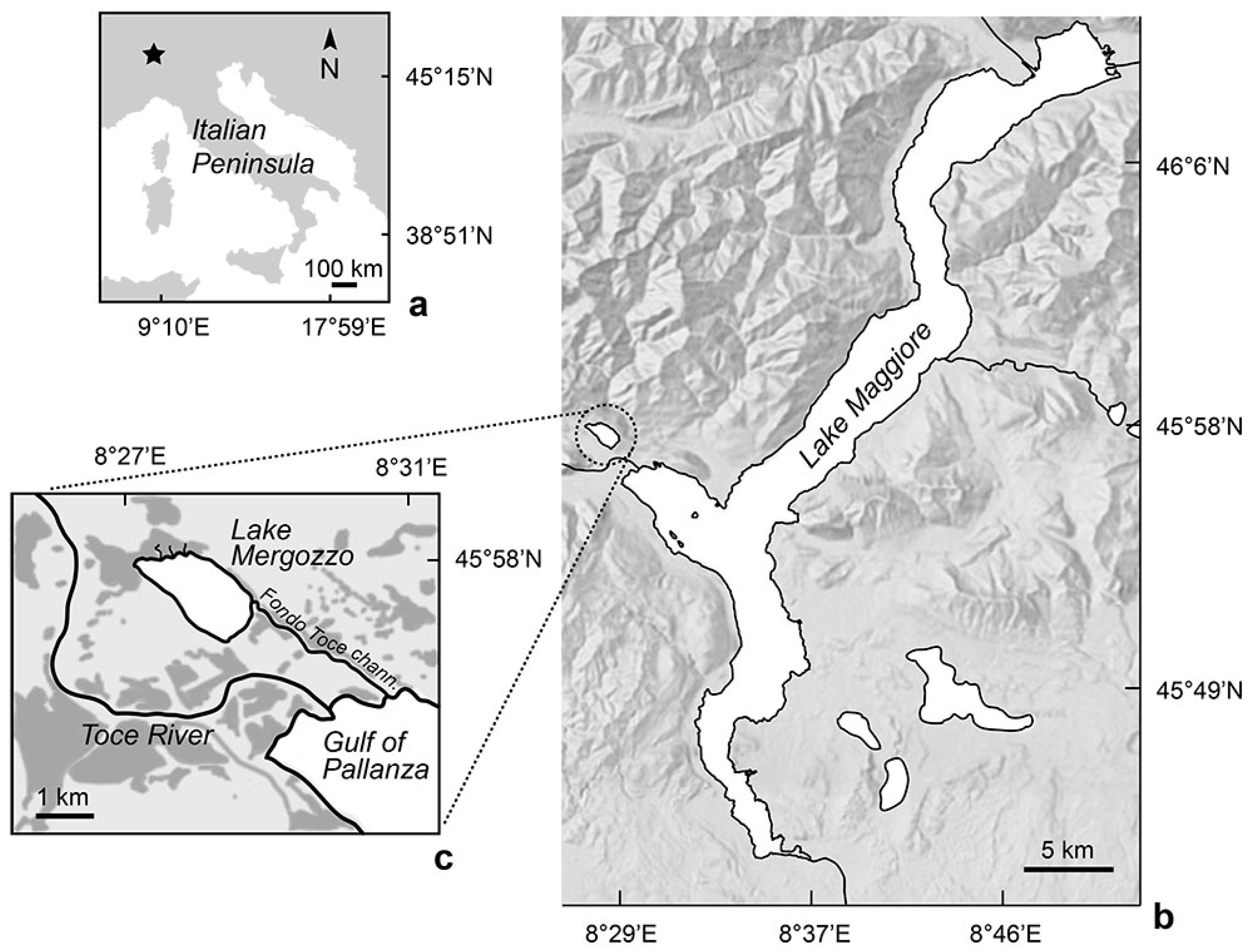
2.1. Study Site

The oligotrophic and relatively deep Lake Mergozzo (total phosphorous concentration ~4 μg L⁻¹, surface area 1.83 km², maximum depth 73 m; [55]) is in the Ticino River basin (193 m above sea level), in north-western Italy (45°57′ N, 8°27′ E; Figure 1). Historically, the lake was the western branch of the nearby Lake Maggiore. About five centuries ago, the two lakes were divided by the progradation of the Toce River delta, whose detritus conoid eventually reached the opposite bank of Lake Maggiore ([57], Figure 1c).

The two lakes are presently connected by a channel; water typically flows from Lake Mergozzo to Lake Maggiore, and in an opposite direction during floods. Lake Mergozzo is a monomictic water body fed by underwater springs, and has a water residence time of about 6 years. Its basin is mainly composed by granitic and metamorphic rocks. The littoral substrate consists of sand and cobble, with a minor fraction of boulder and gravel. Submerged macrophytes are scarce, and a tract of the lake’s southern coast of ~1 km is colonized by a reed bed [Phragmites australis (Cav.) Trin. ex Steud.], near the confluence with the Fondo Toce channel. No commercial fisheries are active in the lake [56], which is included in the protected area ‘Lago di Mergozzo and Montorfano’ (code IT114000013), within the Natura 2000 European network for biodiversity protection, according to the “Habitat Directive” [58].

2.2. Zooplankton, Zoobenthos, and Fish Samples

Carbon sources of lacustrine food webs variably differ from alongshore and offshore environments, due to the differential influence of terrestrial inputs, thus defining littoral and pelagic food webs, respectively [59]. Due to the steep banks and very narrow littoral zone of the lake, we collected zooplankton offshore and zoobenthos alongshore, thus sampling potential fish trophic resources in both littoral and pelagic food webs [60]. Zooplankton was sampled offshore in October 2016, in a single site in the deepest zone of the lake, i.e., at a minimum distance of 500 m from the bank. Two zooplankton samples were collected, using two plankton samplers with a diameter of 59 cm and different filtering efficiency, i.e. with mesh size 450 µm (sample ‘Zoo-450’) and 850 µm (sample ‘Zoo-850’) [61,62]. Each net was hauled vertically 15 times in the 0–50 m layer (total volume filtered ~410 m³). Zoobenthos samples were collected alongshore in October 2016, by kick sampling along a tract of the shore of ~100 m and at a depth of 0–50 cm, using a hand net with 590 μm mesh size. Fish sample surveys were made on 25–27 October and 9, 10 November 2016. Fishes were sampled both offshore, using benthic and mesopelagic gill nets, and alongshore, using an electrofishing device. Each benthic net was 40 m long and 1.5 m high and was made of 16 panels of equal length, with mesh size 5.5–135 mm. Each mesopelagic gill net included two connected sets, A: 27.5 m long and 6 m high, composed of 11 panels with mesh size 8–55 mm knot to knot; and B: 40 m long and 6 m high, composed of 4 panels with mesh size 75 mm, 95 mm, 115 mm, and 135 mm, respectively. Gill nets were distributed following a depth-stratified sampling design, using a sonar (Echosounder, Lowrance HDS7, transducer 50/200 kHz, 300 W). Benthic nets were distributed in 7 strata, at depths of 1.5–2.9 m (A: n = 7), 3.0–5.9 m (B: n = 7), 6.0–11.9 m (C: n = 6), 12.0–19.9 m (D: n = 6), 20.0–34.9 m (E: n = 6), 35.0–50.0 m (F: n = 4), and >50.0 m (G: n = 8). Mesopelagic nets were distributed in 4 strata, at depth intervals of 2–7.9 m (A: n = 4), 8–13.9 m (B: n = 4), 14–19.9 m (C: n = 4), 20–26 m (D: n = 4). Fishes were sampled alongshore (0–1.49 m [63]) from a boat and during daytime with a built-in-frame EL64GII electrofishing device (Scubla Aquaculture, 7000 W, 600 V, DC current) with a copper cathode (width 2 cm, length 300 cm) and a steel ring anode (thickness 0.8 cm, diameter 50 cm). A point abundance sampling electrofishing method was adopted, homogeneously distributing the sampling points (dips) along the coast (~1/80 of perimeter length per dip; PASE, number of dips = 74 [56,63]). All the collected items, including fishes that were euthanized with an overdose of an ethanol suspension of eugenol, were transferred to the laboratory in refrigerated plastic bags.

Fish total length (TL, cm) and wet weight were measured to the nearest mm and g, respectively. Fish species were taxonomically discriminated following [64,65,66]. The taxonomy of the genus Coregonus Linnaeus, 1758 is currently in a state of flux. The only species of Lake Mergozzo is morphologically similar to the Coregonus sp. ‘lavarello’ of the Lake Maggiore [51], possibly either a hybrid species originated from two species introduced from Swiss hatcheries at the end of the 19th century, or likely one of several species introduced in this lake at different times [64,67,68,69,70]). Coregonus sp. ‘bondella’, introduced in Lake Maggiore for the first time in 1950 [51,68,69], is apparently absent from Lake Mergozzo. For these reasons, we will refer to the species of Lake Mergozzo as Coregonus sp. The taxonomy of the genus Salvelinus Richardson, 1836 is also much debated. A species of this genus, often reported in the literature as S. alpinus (Linnaeus, 1758), has plausibly been introduced in northern Italy (Trentino Alto Adige) in the 16th century, then being frequently stocked and translocated in many basins throughout this region [71]. Fertilized eggs of S. alpinus imported from Munich were introduced in Lake Mergozzo by De Filippi in 1862, and in Lake Maggiore in 1910 [69]. We here refer to these populations as Salvelinus umbla, sensu [64]. For electrofishing, sample weights were not available and were inferred using length-weight regressions: M. salmoides [72]; Alburnus arborella (Bonaparte, 1841), L. gibbosus, P. fluviatilis, and R. rutilus [73]; Esox cisalpinus Bianco and Delmastro, 2011, and Scardinius hesperidicus Bonaparte, 1845 [74].

Fish abundance was expressed as relative biomass (%b); relative number (%n); biomass (number of individuals) per unit effort, i.e., BPUE (NPUE) = g (n.)/gill nets’ area, or number of electrofishing dips [g (n.) ind. m⁻² or g (n.) dip⁻¹]. To facilitate comparisons with the published literature, ‘dominant’ fish species in the different types of catch (benthic nets, mesopelagic nets, electrofishing) were defined as the species with abundance > 75 percentile of the biomass and number distributions, using both relative abundances and abundances per unit effort; ‘dominant’ fish species in the total catch were defined using relative abundances.

2.3. Stable Isotope Analysis and Trophic Positions

In the laboratory, all the invertebrates were washed to eliminate detritus; macroinvertebrates were also starved for 24 h to empty their guts. Two subsamples from the Zoo-450 and two from the Zoo-850 zooplankton samples (n = 2; ~1 mg of dry weight each) were used for stable isotope analyses. Other zooplankton and zoobenthos samples were examined under a dissection microscope, identifying animal organisms to the lowest taxonomic level. For macroinvertebrates, isotopes were analyzed from single individuals, i.e., Corbicula fluminea (O.F. Müller, 1774) (Mollusca, Bivalvia; n = 4), and ephemeropteran nymphs (n = 5). For each of the smaller invertebrate taxa (e.g., cladocerans, cyclopoids), several individuals were combined in two pooled samples, to obtain enough material (n = 2; ~1 mg of dry weight each taxon; i.e., ~70–700 individuals) [62]. For fishes, one sample of dorsal muscle was dissected from a subset of the captured individuals (n = 1–9) [75,76,77]. Both invertebrate and fish samples were stored at −20 °C and subsequently freeze-dried. Before further treatment, exoskeletons, valves, and shells of larger invertebrates were removed under a dissection microscope, while smaller organisms were acidified (HCl 1 M) to remove inorganic carbon, and then re-dried (60 °C, 72 h) before analysis. Both invertebrate and fish samples were then finely powdered and homogenized using a ball mill (Fritsch Mini-Mill Pulverisette 23). Subsamples of 0.15–0.25 mg were transferred into cylindrical tin capsules (5 mm × 9 mm, Säntis AnaliticalTM) and oven-dried for at least 24 h at 60 °C.

The isotopic composition of organic carbon and nitrogen was measured in the Stable Isotope Laboratory of the University of Ottawa (G.G. Hatch Lab; [62,76]), using a CE 1110 Elemental Analyser (Vario EL Cube, Elementar, Germany) and a Delta XP Plus Advantage isotope ratio mass spectrometer (Thermo Fisher Scientific, Bremen, Germany) coupled to a ConFlo III interface (Thermo Fisher Scientific, Bremen, Germany). Analytical precision was based on laboratory internal standards, and was usually < 0.2‰ for both δ¹³C and δ¹⁵N. Isotope ratios were expressed as parts per thousand differences (‰) from a standard reference of PeeDee belemnite for carbon and of atmospheric N₂ for nitrogen, according to the equation:

$$({\delta }^{13}\mathrm{C}), \left({\delta }^{15}\mathrm{N}\right)=\left[\left(R_{\mathrm{sample}}/R_{\mathrm{standard}}\right)-1\right]\times 1000$$

(1)

where R is the isotopic ratio: ${}_{}{}^{13}\mathrm{C}/{}_{}{}^{12}\mathrm{C},$or ${}_{}{}^{15}\mathrm{N}/{}_{}{}^{14}\mathrm{N}$.

Lacustrine fish consumers typically acquire nitrogen from pelagic and littoral food webs [78], each characterized by a separate set of primary producers. A two-end member mixing model was thus implemented to estimate the fish trophic positions (TP), assuming no trophic fractionation of carbon and linear mixing [59]. The mean δ¹⁵N signal of the three zooplankton primary consumers Daphnia sp. (Cladocera, Daphniidae), Diaphanosoma brachyurum (Liévin, 1848) (Cladocera, Sididae) and Eubosmina longispina (Leydig, 1860) (Cladocera, Bosminidae) was set as the baseline of the pelagic signal. The mean δ¹⁵N signal of the benthic primary consumer C. fluminea, highly abundant in this system, was set as the baseline of the littoral signal [60]. Although the isotopic signatures of filter-feeding bivalves are generally considered a ‘pelagic’ signature [59,79,80], C. fluminea also consumes large amounts of interstitial detritus by pedal feeding [81], and well represents the benthic signature of the alongshore environment, where it was collected. The TP of each fish species in the two-source food web was thus estimated as [59]:

$$TP=\lambda +\left\{{\delta }^{15}{\mathrm{N}}_{\mathrm{consumer}}-\left[\alpha \times {\delta }^{15}{\mathrm{N}}_{\mathrm{base}-\mathrm{littoral}}+\left(1-\alpha \right)\times {\delta }^{15}{\mathrm{N}}_{\mathrm{base}-\mathrm{pelagic}}\right]\right\}/\Delta n$$

(2)

where λ is the standard trophic level of the baselines [59]; in this case, since our reference organisms are primary consumers, $\lambda$ = 2 [60]. ${\delta }^{15}{\mathrm{N}}_{\mathrm{consumer}}$ is the mean isotopic signature of each fish species; $\Delta n$ is the standard average increase in ${\delta }^{15}\mathrm{N}$ (mean trophic fractionation) from a trophic level to the next one in aquatic food webs (~3.4‰; [59]); α is the proportion of nitrogen in the consumer (fish species) derived from one of the baseline food sources (base‒littoral = littoral baseline; base‒pelagic = pelagic baseline); assuming similar movements of carbon and nitrogen through the food web, α can be estimated using carbon isotopes as [59]:

$$\alpha =\left({\delta }^{13}{\mathrm{C}}_{\mathrm{consumer}}-{\delta }^{13}{\mathrm{C}}_{\mathrm{base}-\mathrm{pelagic}}\right)/\left({\delta }^{13}{\mathrm{C}}_{\mathrm{base}-\mathrm{littoral}}-{\delta }^{13}{\mathrm{C}}_{\mathrm{base}-\mathrm{pelagic}}\right)$$

(3)

In both animals and plants, lipids are depleted in ${}_{}{}^{13}\mathrm{C}$ compared with whole organisms, introducing a bias in the ${\delta }^{13}\mathrm{C}$ of lipid-rich tissues. The lipid content is positively and linearly correlated to $\mathrm{C}:\mathrm{N}$; therefore, the carbon isotopic signature of tissues with $\mathrm{C}:\mathrm{N}$ > 3.5 (i.e., >5% lipid content for aquatic animals) was normalized as [82]:

$${\delta }^{13}{\mathrm{C}}_{\mathrm{normalized}}={\delta }^{13}{\mathrm{C}}_{\mathrm{untreated}}-3.32+0.99\times \left(\mathrm{C}:\mathrm{N}\right)$$

(4)

2.4. Isotopic Niche Metrics, Asymmetrical Overlaps and Statistical Analyses

The isotopic niches of the studied fish species, i.e., the range of carbon and nitrogen signatures by each group of conspecific individuals, were used to evaluate the among-individual component of their realized trophic niches [32,34,83]. Therefore, for each group of conspecifics we calculated the following isotopic niche metrics (SIBER R package [33]; R v. 4.0.0 [84]): carbon range (CR), nitrogen range (NR), mean distance to centroid (CD), standard ellipse corrected area (SEA_c), standard ellipse Bayesian area (SEA_B), mean nearest neighbor distance (MNND) and its standard deviation (SDNND).

CR is the distance between the lowest and highest ${\delta }^{13}\mathrm{C}$ values, evaluating the spectrum of trophic sources of each species; NR is the distance between the lowest and highest ${\delta }^{15}\mathrm{N}$ values, broadly evaluating the range of trophic levels at which each species has been feeding [34]. CD is the average Euclidean distance between the isotopic signature (${\delta }^{13}\mathrm{C}$, ${\delta }^{15}\mathrm{N}$ values) of each conspecific and its centroid, i.e., the point whose coordinates are the means of the respective coordinates of all the points; CD measures the among-individual isotopic diversity of a species, evaluating its trophic diversity. Standard ellipses are in bivariate data the equivalent of SD in univariate data; the standard ellipse area (SEA) is measured as πab, where a and b are the ellipse’s semi-major and semi-minor axes, respectively [33]. SEA_c are sample-size insensitive standard ellipse areas (for n > 3), i.e., the species’ core isotopic niches calculated from the variance and covariance of bivariate isotopic data [34,85,86], evaluating the trophic niche area of a species:

$${\mathrm{SEA}}_{\mathrm{c}}=\mathrm{SEA}\left(n-1\right)\left(n-2\right)-1$$

(5)

where n = number of the species’ individuals.

SEA_B (standard ellipse Bayesian areas) are obtained from standard ellipses constructed using Bayesian inference. The posterior values of the covariance matrix and means of the sampled isotopic signatures are estimated from a set of iterative draws (20,000 iterations) of a Markov chain Monte Carlo (MCMC) simulation, assigning vague normal priors to the means of the isotopic signatures, and a vague Inverse–Wishart prior to the covariance matrix [33]. We then used the Bayesian credible intervals (CI) of the SEA_B, to compare isotopic niche areas among fish species [34]. Within a species, MNND is the mean of the Euclidean distances to each individual signature’s nearest neighbor, i.e., a measure of the density of the individual signatures’ packing in the isotopic space. Species with individuals that are on average more isotopically similar, i.e., with higher isotopic redundancy, would have lower MNND values than species with individuals that are on average more dissimilar. SDNND is the standard deviation of the distances to each signature’s nearest neighbor, i.e., a measure of the variability of the packing of individual signatures. Species with more even distributions of individual signatures, i.e., with higher isotopic evenness, would have lower SDNND values [32]. Isotopic redundancy and isotopic evenness evaluate trophic redundancy and trophic evenness, respectively.

Percentage pairwise asymmetrical overlaps at α levels 0.025, 0.975 CI, and mean asymmetrical overlaps were estimated between sets of 10 Bayesian niche regions, generated for each of two isotopic niche areas (nicheROVER R package, [87,88]). The asymmetrical overlap is a directional metric estimating the probability that an individual signature of Species A is found in the niche area (a) of Species B (pAB); this probability is different than the probability that an individual signature of Species B is found in the niche area of Species A (pBA), since A and B typically have different niche areas (aA, aB). Therefore, if aB > aA, then pAB > pBA. Within the fish subsample used for SIA, fish species with s < 4 were eliminated from the analyses of isotopic niche metrics and asymmetrical overlaps.

Mann–Whitney U tests were performed between fish NS and NNS for TP, isotopic niche metrics, and both biomass (BPUE) and number (NPUE) of fishes per unit effort (all sampling methods). These statistical tests were performed in PAST v.4© [89].

3. Results

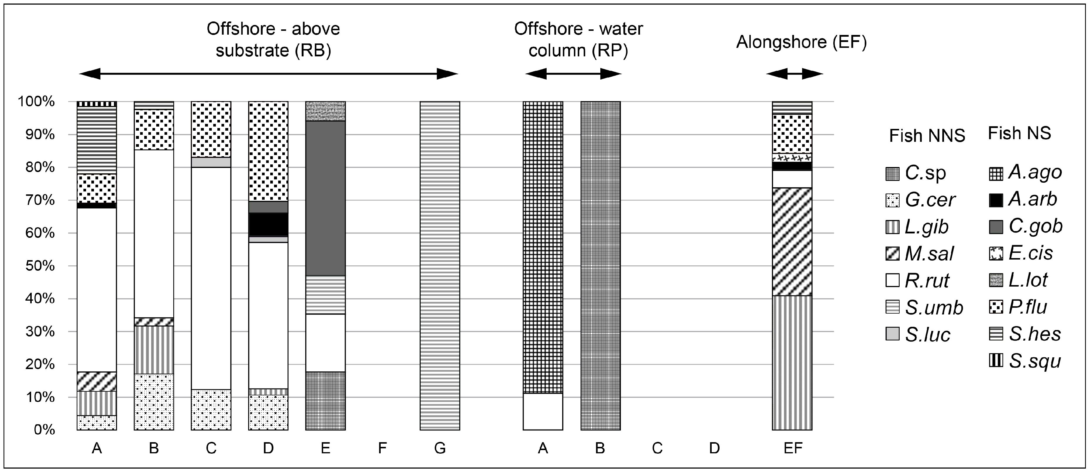
3.1. Zooplankton, Zoobenthos, and Fish Samples

Zooplankton samples collected offshore contained Bythotrephes longimanus Leydig, 1860 (Cladocera, Cercopagididae); Cyclopoida (Copepoda); Daphnia sp.; D. brachyurum; E. longispina; and Leptodora kindtii (Focke, 1884) (Cladocera, Leptodoridae). Zoobenthos samples collected alongshore only contained ephemeropteran nymphs (Insecta, Ephemeroptera) and bivalves (C. fluminea).

Benthic fish nets collected 72%b and 74%n of the total catch; mesopelagic nets and electrofishing yielded smaller catches (7%b and 4%n; 22%b and 22%n, respectively) (StotMET,

Table 1. Fish catches sampled in Lake Mergozzo in 2016. TL = total length; Fish NNS = fish non-native species; Fish NS = fish native species; RBb (n) = biomass (number) collected with benthic gill nets; RPb (n) = biomass (number) collected with mesopelagic gill nets; EFb (n) = biomass (number) collected with electrofishing; RB%b (%n), RP%b (%n), EF%b (%n) = percentage biomass (number) collected with the different sampling methods, relative to the biomass (number) of all the species collected with the corresponding sampling method; TOTb (TOTn) = total biomass (number) collected with all sampling methods; TOT%b (TOT%n) = percentage total biomass (number) relative to the total sample; StotMET = sub-totals of each type of sampling method, and percentages relative to the total sample; in bold: values >75 percentile of the fish NNS and fish NS corresponding distributions (‘dominant’ species by abundance). See Appendix A, Table A1 for mean TL, and mean BPUE, NPUE.

		TL (cm)	Biomass								Number of Fish Individuals
Species	Common Name	Range	RBb	RB%b	RPb	RP%b	EFb	EF%b	TOTb	TOT%b	RBn	RB%n	RPn	RP%n	EFn	EF%n	TOTn	TOT%n
Fish NNS§
Coregonus sp.	European whitefish	8.4–43.6	29	0.1	2024	93.4	0	0.0	2053	6.3	3	1.2	4	30.8	0	0.0	7	2.1
G. cernua	Ruffe	5.2–17.8	751	3.2	0	0.0	0	0.0	751	2.3	24	9.6	0	0.0	0	0.0	24	7.1
L. gibbosus	Pumpkinseed	4.6–25.0	537	2.3	0	0.0	1380	19.3	1917	5.9	12	4.8	0	0.0	31	40.8	43	12.7
M. salmoides	Largemouth bass	5.4–30.5	537	2.3	0	0.0	2234	31.2	2771	8.5	5	2.0	0	0.0	25	32.9	30	8.8
R. rutilus	Roach	5.8–33.0	10,657	45.7	22	1.0	54	0.8	10,733	32.9	127	50.8	1	7.7	4	5.3	132	38.9
S. umbla	Char	16.3–28.3	520	2.2	0	0.0	0	0.0	520	1.6	5	2.0	0	0.0	0	0.0	5	1.5
S. lucioperca	Pikeperch	37.4–73.0	5080	21.8	0	0.0	0	0.0	5080	15.6	3	1.2	0	0.0	0	0.0	3	0.9
Fish NS
A. agone	Shad	10.7–13.0	0	0.0	121	5.6	0	0.0	121	0.4	0	0.0	8	61.5	0	0.0	8	2.4
A. arborella	Bleak	5.0–8.8	19	0.1	0	0.0	4	0.1	23	0.1	5	2.0	0	0.0	2	2.6	7	2.1
C. gobio	Bullhead	4.0–9.7	46	0.2	0	0.0	0	0.0	46	0.1	10	4.0	0	0.0	0	0.0	10	2.9
E. cisalpinus	Southern pike	56.0, 65.0	0	0.0	0	0.0	2975	41.6	2975	9.1	0	0.0	0	0.0	2	2.6	2	0.6
L. lota	Burbot	31.3	161	0.7	0	0.0	0	0.0	161	0.5	1	0.4	0	0.0	0	0.0	1	0.3
P. fluviatilis	Perch	6.5–41.1	3554	15.2	0	0.0	297	4.2	3851	11.8	39	15.6	0	0.0	9	11.8	48	14.2
S. hesperidicus	Italian rudd	15.1–33.0	1304	5.6	0	0.0	205	2.9	1509	4.6	15	6.0	0	0.0	3	3.9	18	5.3
S. squalus	Italian chub	24.6	144	0.6	0	0.0	0	0.0	144	0.4	1	0.4	0	0.0	0	0.0	1	0.3
StotMET			23,339	71.5	2167	6.6	7149	21.9	32,655	100.0	250	73.7	13	3.8	76	22.4	339	100.0

^§ biomass of fish NNS = 23,825 g (relative to total biomass = 73.0%b). Number of fish NNS = 244 (relative to total number = 72.0%n).

). A total of 339 fishes were collected, including 7 fish NNS: Coregonus sp., G. cernua, L. gibbosus, M. salmoides, R. rutilus, S. umbla, and S. lucioperca; and 8 fish NS: Alosa agone (Scopoli, 1786), A. arborella, Cottus gobio Linnaeus, 1758, E. cisalpinus, L. lota, P. fluviatilis, S. hesperidicus, Squalius squalus (Bonaparte, 1837) (Table 1). Fish NNS make up most of the total fish sample, both in biomass (23.8·103 g, 73%b) and numbers (n = 244, 72%n) (Table 1).

Both mean BPUE and NPUE of fish-NNS electrofishing and benthic catches are significantly larger than those of fish NS (Mann–Whitney U tests, U = 48,524–145,596, p < 0.001); the average electrofishing (benthic) catch per unit effort of fish NNS was 1.2 (4) times heavier and 4 (3) times more numerous than that of fish NS (Appendix A,

Table A1. Fishes collected in Lake Mergozzo by benthic (RB) gill nets, mesopelagic (BP) gill nets, and electrofishing (EF), in 2016; BPUE (NPUE) = fish biomass (number of individuals) per unit effort; TL (cm) = total length; Fish NS = fish native species; Fish NNS = fish non-native species; all values: mean ± SD, or values, if n < 3. Overall means ± SD: means ± SD of the total fish NNS (NS) samples, for each type of sampling method; Grand means: means ± SD of the total fish sample, for each type of sampling method; in bold: values > 75 percentile of the fish NNS and fish NS corresponding distributions (‘dominant’ species by abundance). See Table 1 for TL ranges, fish numbers and weights.

	TL (cm)				BPUE (g ind. m−2 or g ind. dip−1)				NPUE (n. ind. m−2 or n. ind. dip−1)
Fish Species	RB	RP	EF		RB	RP	EF		RB	RP	EF
Fish NNS
Coregonus sp.	11.1 ± 2.3	39.1 ± 4.3	-		0.01 ± 0.05	0.312 ± 0.863	0.00 ± 0.00		0.0011 ± 0.0056	0.0006 ± 0.0017	0.00 ± 0.00
G. cernua	12.3 ± 3.3	-	-		0.26 ± 0.53	0.000 ± 0.000	0.00 ± 0.00		0.0087 ± 0.0159	0.0000 ± 0.0000	0.00 ± 0.00
L. gibbosus	13.2 ± 2.3	-	11.5 ± 3.8		0.2 ± 0.52	0.000 ± 0.000	18.65 ± 77.31		0.0045 ± 0.0104	0.0000 ± 0.0000	0.42 ± 1.10
M. salmoides	19.5 ± 6.2	-	13.9 ± 7.9		0.20 ± 0.70	0.000 ± 0.000	30.19 ± 104.70		0.0019 ± 0.0064	0.0000 ± 0.0000	0.34 ± 0.69
R. rutilus	17.4 ± 6.8	13.8	9.7 ± 3.9		4.04 ± 6.74	0.003 ± 0.014	0.73 ± 4.57		0.0481 ± 0.0762	0.0002 ± 0.0006	0.05 ± 0.23
S. umbla	22.8 ± 4.4	-	-		0.20 ± 0.62	0.000 ± 0.000	0.00 ± 0.00		0.0019 ± 0.0054	0.0000 ± 0.0000	0.00 ± 0.00
S. lucioperca	56.0, 65.0	-	-		1.92 ± 11.21	0.000 ± 0.000	0.00 ± 0.00		0.0011 ± 0.0056	0.0000 ± 0.0000	0.00 ± 0.00
Overall means ± SD					0.98 ± 5.11	0.045 ± 0.336	7.08 ± 50.25		0.0096 ± 0.0337	0.0001 ± 0.0007	0.12 ± 0.52
Fish NS
A. agone	-	11.9 ± 0.7	-		0.00 ± 0.00	0.019 ± 0.035	0.00 ± 0.00		0.0000 ± 0.0000	0.0012 ± 0.0024	0.00 ± 0.00
A. arborella	8.2 ± 0.7	-	-		0.01 ± 0.03	0.000 ± 0.000	0.05 ± 0.37		0.0019 ± 0.0082	0.0000 ± 0.0000	0.03 ± 0.16
C. gobio	7.1 ± 2.0	-	-		0.02 ± 0.06	0.000 ± 0.000	0.00 ± 0.00		0.0038 ± 0.0134	0.0000 ± 0.0000	0.00 ± 0.00
E. cisalpinus	-	-	-		0.00 ± 0.00	0.000 ± 0.000	40.2 ± 248.77		0.0000 ± 0.0000	0.0000 ± 0.0000	0.03 ± 0.16
L. lota	31.3	-	-		0.06 ± 0.40	0.000 ± 0.000	0.00 ± 0.00		0.0004 ± 0.0025	0.0000 ± 0.0000	0.00 ± 0.00
P. fluviatilis	16.1 ± 8.7	-	12.4 ± 3.9		1.35 ± 3.48	0.000 ± 0.000	4.01 ± 20.24		0.0148 ± 0.0292	0.0000 ± 0.0000	0.12 ± 0.37
S. hesperidicus	19.1 ± 4.2	-	16.9 ± 2.0		0.49 ± 1.91	0.000 ± 0.000	2.77 ± 14.19		0.0057 ± 0.0262	0.0000 ± 0.0000	0.04 ± 0.2.0
S. squalus	24.6	-	-		0.05 ± 0.36	0.000 ± 0.000	0.00 ± 0.00		0.0004 ± 0.0025	0.0000 ± 0.0000	0.00 ± 0.00
Overall means ± SD					0.25 ± 1.47	0.002 ± 0.014	5.88 ± 88.83		0.0034 ± 0.0156	0.0002 ± 0.0009	0.03 ± 0.17
Grand means					0.59 ± 3.67	0.022 ± 0.230	6.44 ± 73.36		0.0063 ± 0.0258	0.0001 ± 0.0008	0.07 ± 0.38

). Nine fish species dominate different catches. The total catch is dominated in relative biomass by R. rutilus, S. lucioperca, P. fluviatilis, and E. cisalpinus (in descending order); and in relative number by R. rutilus, P. fluviatilis, L. gibbosus, and M. salmoides (Table 1). Considering both relative abundance and mean catches per unit efforts (BPUE, NPUE), benthic catches are dominated in biomass by R. rutilus, S. lucioperca, P. fluviatilis, and S. hesperidicus; and in number by R. rutilus, P. fluviatilis, G. cernua, and S. hesperidicus. Mesopelagic catches are dominated in biomass by Coregonus sp., A. agone, and R. rutilus, and in number by A. agone, Coregonus sp., and R. rutilus. Electrofishing catches are dominated in biomass by E. cisalpinus, M. salmoides, L. gibbosus, and P. fluviatilis; and in number by L. gibbosus, M. salmoides, P. fluviatilis, and R. rutilus (Table 1, Appendix A, Table A1). The only species recorded with all types of sampling methods was R. rutilus (Table 1).

The fish depth distribution (relative abundances by depth; Figure 2, Appendix A, Figure A2) provides an overview of the habitat distribution of the fishes sampled alongshore (electrofishing sample); offshore, above the bottom (benthic nets sample); and offshore, in the water column (mesopelagic nets sample).

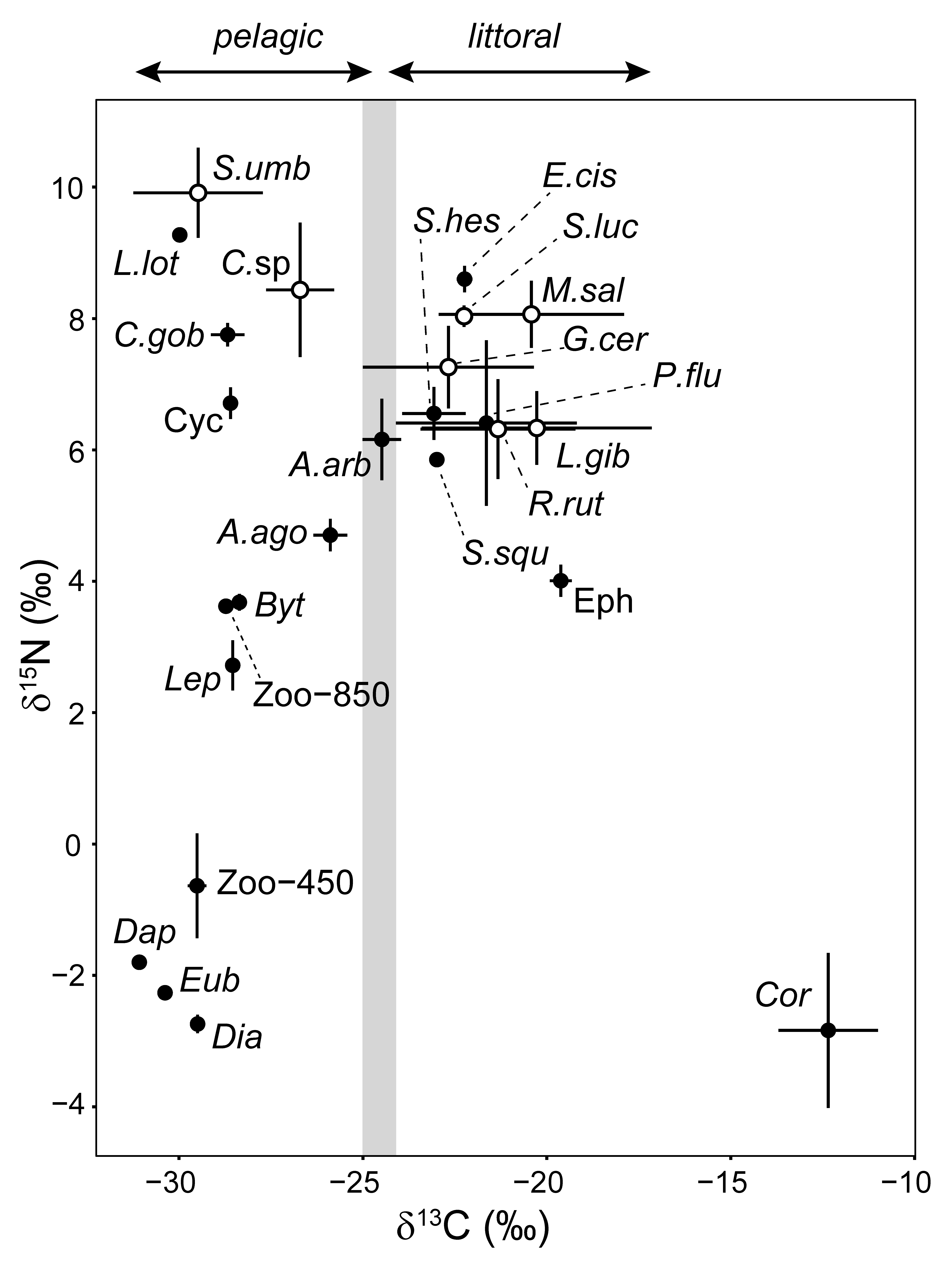
3.2. Stable Isotope Analysis and Trophic Positions

Mean ${\delta }^{13}\mathrm{C}$ values of the potential trophic sources range from −31.1‰ of Daphnia sp. to −12.3‰ of C. fluminea; mean ${\delta }^{15}\mathrm{N}$ values range from −2.8‰ of C. fluminea to 6.7‰ of Cyclopoida (

Table 2. Isotopic signatures of the potential trophic resources of the studied fishes; δ¹⁵N and δ¹³C: mean ± SD‰; when the number of subsamples < 3, values are reported; AS = alongshore sample (zoobenthos), OS = offshore sample (zooplankton); Zoo-450 = zooplankton sample ≥ 450 μm; Zoo-850 = zooplankton sample ≥ 850 μm.

Species	Sample	δ13C	δ15N
Corbicula fluminea	AS	−12.35 ± 1.35	−2.84 ± 1.18
Ephemeroptera	AS	−19.62 ± 0.30	4.01 ± 0.25
Bythotrephes longimanus	OS	−28.43, −28.29	3.77, 3.59
Cyclopoida	OS	−28.73, −28.47	6.88, 6.54
Daphnia sp.	OS	−31.08	−1.80
Diaphanosoma brachyurum	OS	−29.47, −29.52	−2.64, −2.84
Eubosmina longispina	OS	−30.39, −30.37	−2.27, −2.26
Leptodora kindtii	OS	−28.61, −28.47	2.45, 2.99
Zoo-450	OS	−29.33, −29.69	−0.07, −1.20
Zoo-850	OS	−28.82, −28.63	3.57, 3.67

).

Mean ${\delta }^{13}\mathrm{C}$ values of the fish species range from −29.5‰ of S. umbla to −20.3‰ of L. gibbosus; mean ${\delta }^{15}\mathrm{N}$ values range from 4.5‰ of A. agone to 9.9‰ of S. umbla (

Table 3. Isotopic signatures and trophic positions (TP) of the fish species; ss = number of subsamples used for SIA; ${\delta }^{15}\mathrm{N}$ and ${\delta }^{13}\mathrm{C}$ = mean ± SD ‰; when ss < 3, values are reported.

Species	ss	δ15N	δ13C	TP
Fish NNS
Coregonus sp.	4	8.17 ± 1.26	−26.56 ± 0.99	4.94
G. cernua	9	7.26 ± 0.63	−22.68 ± 2.32	5.01
L. gibbosus	5	6.33 ± 0.56	−20.27 ± 3.13	4.78
M. salmoides	5	8.06 ± 0.51	−20.42 ± 2.52	5.22
R. rutilus	8	6.32 ± 0.76	−21.33 ± 2.11	4.59
S. umbla	4	9.90 ± 0.69	−29.48 ± 1.76	5.75
S. lucioperca	2	7.92, 8.15	−22.24, −22.26	4.92
Fish NS
A. agone	4	4.49 ± 0.39	−26.06 ± 0.22	4.12
A. arborella	4	6.15 ± 0.62	−24.48 ± 0.52	2.83
C. gobio	4	7.75 ± 0.18	−28.68 ± 0.46	3.29
E. cisalpinus	2	8.46, 8.75	−22.00, −22.30	5.06
L. lota	1	9.67	−29.98	5.15
P. fluviatilis	7	6.40 ± 1.26	−21.64 ± 2.46	4.95
S. hesperidicus	5	6.55 ± 0.40	−23.07 ± 0.86	4.61
S. squalus	1	5.85	−22.99	4.11

). Along the ${\delta }^{13}\mathrm{C}$ axis, Zoo-450, Zoo-850, cladocerans and copepods are closer to the pelagic baseline (Daphnia sp., plus D. brachyurum, plus E. longispina), while ephemeropterans are closer to the littoral baseline (C. fluminea) (Section 2.3; Figure 3).

Therefore, potential fish trophic resources form two isotopically distinct groups: those collected in the alongshore environment, with enriched carbon signatures (${\delta }^{13}\mathrm{C}$> −20‰; group A: littoral food web); and those collected in the offshore environment, with depleted carbon signatures (${\delta }^{13}\mathrm{C}$< −28‰; group B: pelagic food web) (Table 2; Figure 3). Along the ${\delta }^{13}\mathrm{C}$ axis, the signatures of group A are closer to those of fishes with relatively enriched carbon signatures, that likely fed in the littoral food web (L. gibbosus, M. salmoides, R. rutilus, P. fluviatilis, E. cisalpinus, S. lucioperca, S. squalus, and S. hesperidicus, in order of decreasing ${\delta }^{13}\mathrm{C}$; mean ${\delta }^{13}\mathrm{C}$ −20.3‰ to −23.1‰). The signatures of group B are closer to those of fish species with relatively depleted carbon signatures, that likely fed in the pelagic food web (A. agone, Coregonus sp., C. gobio, S. umbla, and L. lota; mean ${\delta }^{13}\mathrm{C}$ −26.1‰ to −30.0‰) (Table 3; Figure 3). G. cernua and A. arborella apparently fed in both food webs (mean ${\delta }^{13}\mathrm{C}$ −22.7‰, −24.5‰, respectively). Mean ${\delta }^{13}\mathrm{C}$ signatures of fish NNS and NS are broadly overlapped, ranging from −29.5‰ (S. umbla) to −20.3‰ (L. gibbosus) in the former, and from −30.0‰ (L. lota) to −21.6‰ (P. fluviatilis) in the latter (Table 3; Figure 3).

Mean ${\delta }^{15}\mathrm{N}$ signatures of potential fish food sources define two distinct groups: (i) ephemeropterans, the pooled larger zooplankton sample (Zoo-850), and the zooplankters B. longimanus, Cyclopoida, plus L. kindtii, with more enriched ${\delta }^{15}\mathrm{N}$ signatures; and (ii) C. fluminea, the pooled smaller zooplankton sample (Zoo-450), and the zooplankters E. longispina, Daphnia sp., plus D. brachyurum, with more depleted ${\delta }^{15}\mathrm{N}$ signatures (Table 2; Figure 3). Mean ${\delta }^{15}N$ signatures of fish NNS and NS are broadly overlapped, ranging from 6.3‰ (R. rutilus) to 9.9‰ (S. umbla) in the former, and from 4.5‰ (A. agone) to 9.7‰ (L. lota) in the latter (Table 3; Figure 3). The fish trophic positions (TP; Table 3; Appendix A, Figure A1) range from 2.8 of A. arborella to 5.7 of S. umbla. Fish NNS have non-significantly higher mean TP than fish NS (TP = 5.03 ± 0.37 SD and TP = 4.27 ± 0.85 SD, respectively; Mann–Whitney test, U = 15, p = 0.15; Table 3; Appendix A, Figure A1). If TP values are divided into three equal intervals, fish NNS include six species with higher TP (TP ≥ 4.80: S. umbla, M. salmoides, G. cernua, Coregonus sp., and S. lucioperca, in descending order), and two species with intermediate TP (4.80 > TP > 3.80: L. gibbosus, R. rutilus). Fish NS include three species with higher TP (L. lota, E. cisalpinus, P. fluviatilis), three species with intermediate TP (S. hesperidicus, A. agone, S. squalus), and two species with lower TP (TP ≤ 3.80: C. gobio, A. arborella).

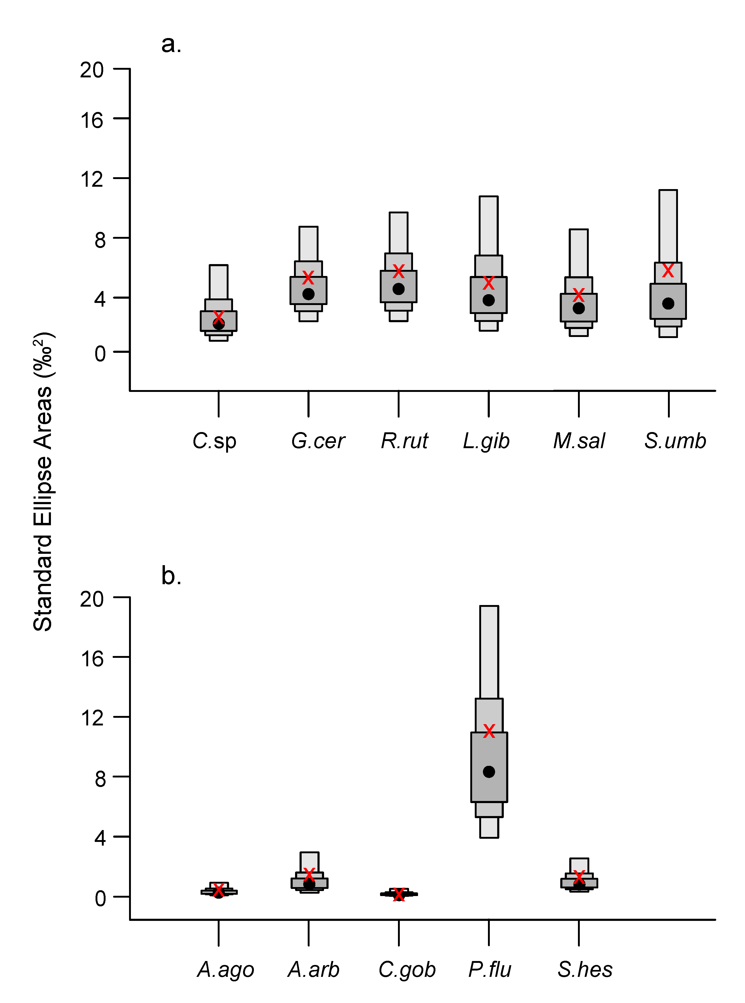
3.3. Isotopic Niche Metrics and Overlaps

Fish NNS have significantly higher values of carbon range (CR), mean nearest neighbor distance (MNND) and SD of the nearest neighbor distance (SDNND) than fish NS; and non-significantly higher values of NR, CD, SEA_c and SEA_B (

Table 4. Isotopic niche metrics for non-native and native fish species (Fish NNS, Fish NS, respectively): ss = number of subsamples used for SIA; CR = carbon range (‰); NR = nitrogen range (‰); CD = mean distance to centroid (‰); SEA_c = standard ellipse corrected area (‰²); SEA_B = standard ellipse Bayesian area (‰²); MNND = mean nearest neighbor distance (‰); SDNND = standard deviation of nearest neighbor distance (‰); Mann–Whitney U tests between fish NNS and NS: * p < 0.05; ** p < 0.01; fish species with < 4 analyzed specimens are not included.

Species	ss	CR *	NR	CD	SEAc	SEAB	MNND *	SDNND **
Fish NNS
Coregonus sp.	4	2.22	2.28	1.02	2.70	2.52	0.94	0.86
G. cernua	9	7.57	2.10	1.98	5.22	5.11	0.90	0.98
L. gibbosus	5	7.88	1.47	2.32	4.86	5.00	1.75	2.00
M. salmoides	5	6.08	1.36	1.85	3.99	4.32	1.48	1.88
R. rutilus	8	6.11	2.37	1.88	5.68	5.56	0.96	0.74
S. umbla	4	4.13	1.47	1.45	5.42	5.79	1.46	0.70
Mean values ± SD		5.67 ± 2.15	1.84 ± 0.46	1.75 ± 0.45	4.64 ± 1.12	4.72 ± 1.19	1.25 ± 0.36	1.19 ± 0.59
Fish NS
A. agone	4	1.12	0.52	0.42	0.46	1.13	0.53	0.10
A. arborella	4	1.28	1.32	0.68	1.47	2.67	0.76	0.28
C. gobio	4	0.94	0.43	0.41	0.16	0.07	0.26	0.12
P. fluviatilis	7	6.23	3.50	2.40	11.69	12.34	1.20	0.63
S. hesperidicus	5	1.90	0.96	0.81	1.39	1.19	0.62	0.18
Mean values		2.29 ± 2.23	1.35 ± 1.26	0.94 ± 0.83	3.03 ± 4.87	3.48 ± 5.04	0.67 ± 0.35	0.26 ± 0.22

, Appendix A, Figure A1). The fish NS P. fluviatilis has values of the isotopic metrics closer to average fish NNS values (except SDNND; Appendix A, Figure A1), exhibiting the widest nitrogen range (NR), the highest average trophic diversity (CD), and the largest niche areas (SEA_c, SEA_B) of all the fish species (Table 4, Appendix A, Figure A1).

Pairwise mean asymmetrical overlaps provide conservative estimates of trophic niche overlaps ([87];

Table 5. Credible intervals (0.975, 0.025 CI) and means (Mean) of percentage asymmetrical overlaps (%) between isotopic niche regions of the analyzed fish sample; in each pairwise comparison within a row, the percentage indicates the proportion of the row’s species niche being asymmetrically overlapped with another species’ niche in a column; NA = not assigned; fish species with < 4 analyzed specimens are not included; in bold: mean overlaps ≥ 70% (arbitrary cut-off), and grand-mean overlaps of the corresponding species in columns. See Figure 3 for species abbreviations.

		A.arb	A.ago	C.gob	C.sp	G.cer	L.gib	M.sal	P.flu	R.rut	S.umb	S.hes
A.arb	0.025 CI	NA	0.00	0.00	0.00	8.12	0.00	0.00	29.22	5.55	0.00	2.34
	0.975 CI	NA	22.56	0.00	82.45	99.88	86.53	12.12	100.00	100.00	0.00	90.78
	Mean	NA	2.95	0.04	16.94	56.69	32.31	1.82	89.59	75.69	0.26	41.16
A.ago	0.025 CI	0.00	NA	0.00	0.00	0.00	0.00	0.00	0.00	0.00	0.00	0.00
	0.975 CI	84.87	NA	0.00	15.89	6.0	0.00	0.00	100.00	100.00	0.00	5.38
	Mean	11.08	NA	0.00	1.11	1.04	0.22	0.01	35.02	22.51	0.00	1.05
C.gob	0.025 CI	0.00	0.00	NA	0.00	0.00	0.00	0.00	0.00	0.00	0.00	0.00
	0.975 CI	0.00	0.00	NA	19.11	100.00	100.00	0.00	100.00	7.77	94.33	0.00
	Mean	0.05	0.00	NA	2.52	24.48	11.23	0.80	11.07	1.26	5.87	0.03
C.sp	0.025 CI	0.00	0.00	0.00	NA	3.64	0.00	0.00	0.00	0.00	0.00	0.00
	0.975 CI	22.98	22.34	1.13	NA	86.28	53.65	64.87	96.34	46.47	73.81	13.55
	Mean	4.03	0.10	0.08	NA	40.02	11.08	9.82	28.84	6.38	21.62	1.72
G.cer	0.025 CI	1.94	1.00	0.00	1.34	NA	11.89	4.54	56.44	21.32	0.00	7.52
	0.975 CI	39.76	39.56	1.16	27.43	NA	84.34	66.99	100.00	96.77	6.66	58.99
	Mean	11.15	0.05	0.25	10.39	NA	41.60	25.45	85.02	58.91	0.74	24.61
L.gib	0.025 CI	0.00	0.00	0.00	0.00	19.46	NA	0.00	48.55	37.44	0.00	5.03
	0.975 CI	25.8	25.56	1.34	17.34	96.02	NA	33.23	100.00	99.99	2.55	50.05
	Mean	6.39	0.01	0.16	4.07	58.87	NA	2.93	83.26	74.25	0.17	22.12
M.sal	0.025 CI	0.00	0.00	0.00	0.00	7.57	0.00	NA	12.39	0.00	0.00	0.00
	0.975 CI	11.28	0.00	0.00	12.33	97.33	25.71	NA	100.00	90.06	12.25	15.47
	Mean	0.83	0.00	0.01	2.00	57.29	2.66	NA	67.35	28.61	1.29	1.42
P.flu	0.025 CI	1.00	0.00	0.00	0.00	21.56	17.45	2.45	NA	31.27	0.00	6.65
	0.975 CI	27.43	4.65	0.00	16.56	85.33	68.44	40.89	NA	94.84	4.56	46.43
	Mean	8.05	0.58	0.06	3.69	52.23	38.95	14.70	NA	64.60	0.49	18.69
R.rut	0.025 CI	1.00	0.00	0.00	0.00	22.43	26.78	0.00	68.33	NA	0.00	6.77
	0.975 CI	31.85	3.76	0.00	14.88	95.44	86.54	36.55	100.00	NA	0.00	54.72
	Mean	8.72	0.66	0.02	2.25	59.54	54.76	9.58	91.85	NA	0.15	24.67
S.umb	0.025 CI	0.00	0.00	0.00	0.00	0.00	0.00	0.00	0.00	0.00	NA	0.00
	0.975 CI	0.00	0.00	1.44	51.22	10.55	3.79	36.72	24.44	0.00	NA	0.00
	Mean	0.02	0.00	0.09	15.19	1.15	0.25	2.24	2.29	0.06	NA	0.01
S.hes	0.025 CI	2.99	0.00	0.00	0.00	47.43	25.11	0.00	88.91	55.38	0.00	NA
	0.975 CI	89.64	1.85	0.00	34.33	100.00	100.00	29.45	100.00	100.00	0.00	NA
	Mean	26.47	0.18	0.01	3.97	88.08	73.53	3.34	98.61	93.84	0.18	NA
Grand-mean overlaps		7.68	0.18	0.08	5.02	42.52	26.03	7.65	55.92	38.94	3.39	10.48

). The niches of A. arborella, G. cernua, L. gibbosus, R. rutilus, and S. hesperidicus are broadly overlapped (arbitrary cut-off ≥ 70%) with the niche of the fish NS P. fluviatilis; the niches of A. arborella, L. gibbosus, and S. hesperidicus are overlapped with that of R. rutilus; and the niche of S. hesperidicus is also overlapped with those of G. cernua and L. gibbosus (Table 5).

Except S. umbla, P. fluviatilis, R. rutilus, G. cernua, and L. gibbosus are also the fish species with the largest isotopic niches (Figure 4 and Figure 5); their signatures have the highest average probability to be contained in the niche of another species (grand means: 56%, 39%, 42%, and 26%, respectively; Table 5). In particular, four broad overlaps occurred between the larger niche of a fish NNS and the smaller niche of a fish NS (i.e., R. rutilus > A. arborella; G. cernua, L. gibbosus, R. rutilus > S. hesperidicus); two overlaps between two fish NS (i.e., P. fluviatilis > A. arborella, S. hesperidicus); one overlap between two fish NNS (R. rutilus > L. gibbosus); and three overlaps between the larger niche of a fish NS and the smaller niche of a fish NNS (P. fluviatilis > G. cernua, L. gibbosus, R. rutilus).

4. Discussion

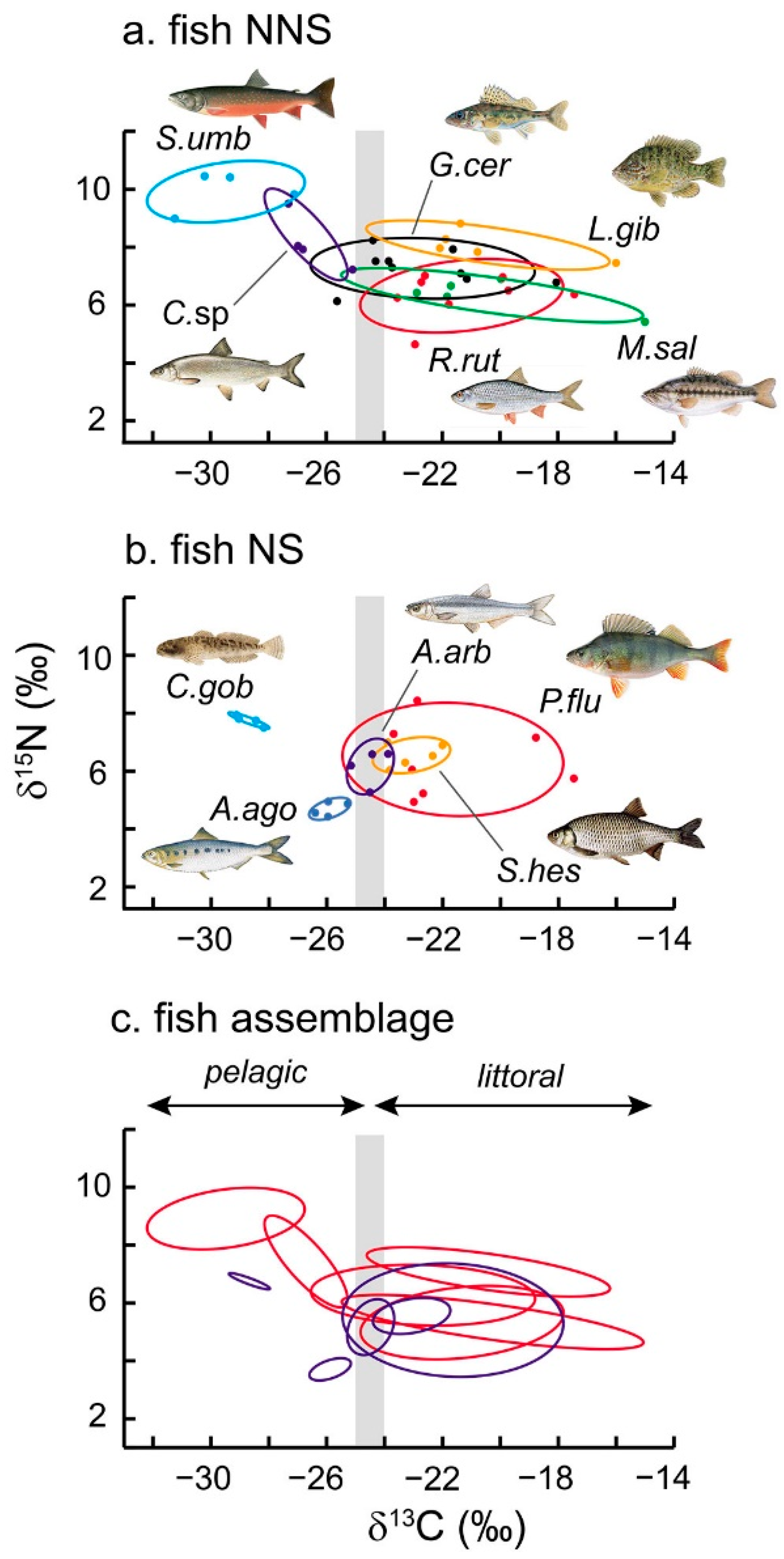
4.1. The Fish Community of Lake Mergozzo

The higher abundance of fish NNS in Lake Mergozzo clearly describes the remarkable change in community structure caused by fish introductions. In a study conducted in 2010 [56] fish NS, fish NNS introduced after 1950, and fish NNS introduced before 1950 made up 40%, 50%, and 10% of the total catch by biomass; and 30%, 61%, 9% by numbers, respectively. In our sample, fish NS, fish NNS introduced after 1950, and fish NNS introduced before 1950 made up 27%, 51%, 22% of the total catch by biomass; and 28%, 47%, 25% by numbers, respectively. This suggests a recent relative increase in the abundance of historically introduced fish NNS (e.g., M. salmoides, L. gibbosus). Among the fish NNS of this study, G. cernua, R. rutilus and S. lucioperca were first recorded in Lake Mergozzo in 2010 [55] following their appearance in the neighboring Lake Maggiore with a delay of 10–30 years (Volta, unpublished data; [54,90]). All other fish NNS were introduced before 1950, mostly in the 19th century [52,53,56].

In the 2010 survey by Volta et al. [56], the total catch was dominated in relative number by R. rutilus, P. fluviatilis, S. hesperidicus, G. cernua, and M. salmoides. In the first ichthyological survey of Lake Mergozzo, made only two decades before [51], G. cernua, R. rutilus, and S. lucioperca were not found, and the total catch was dominated in relative number by S. hesperidicus, Rutilus rubilio (Bonaparte, 1837) [= Sarmarutilus rubilio (Bonaparte, 1837)], P. fluviatilis, and Coregonus species. Within the limitations of sampling biases and different sampling methods, qualitative comparisons between the 1994 survey and both our dataset and the 2010 survey suggest that changes in the relative species abundance in Lake Mergozzo were dramatic. This scenario mirrors other lakes and rivers in northern Italy, once more indicating the rising tide of warm-water tolerant and omnivorous species in the Po River Basin [56,91,92,93,94].

4.2. Foraging Habitats and Food Ecology

The large difference in ${\delta }^{13}\mathrm{C}$ signatures between potential trophic resources sampled alongshore and offshore supports the distinction between a littoral and a pelagic food webs, spatially separated in alongshore and offshore environments, respectively [59,78]. The isotopic signatures of both fish NS and NNS, and of their potential food sources are distributed along this whole ${\delta }^{13}\mathrm{C}$ gradient. In each environment, isotopic signatures evaluated foraging habitats throughout the entire water column; consistently, carbon signatures suggest that several pelagic (A. agone), demersal (Coregonus sp., S. umbla) and benthic fishes (C. gobio, L. lota) mainly foraged offshore in Lake Mergozzo, in the pelagic food web. The carbon signatures of other demersal species (e.g., L. gibbosus, M. salmoides, R. rutilus) suggest that these mainly foraged alongshore, along the narrow littoral zone of the lake’s steep banks and in the reed bed along its southern bank, in the littoral food web. The epipelagic A. arborella and the demersal G. cernua, known to perform feeding migrations between habitats at different depths, apparently foraged in both food webs (Appendix A,

Table A2. Foraging habitats and food ecology of the studied fish species in the literature. Status: NS = fish native species; NNS = fish non-native species in Lake Mergozzo; TL = total length range; underlined: main food items, considering the size range and other characteristics of the population of Lake Mergozzo; in parentheses: less important food items; see also Table 1, Appendix A, Table A1.

Species	TL (cm)	Status	Common Food Source	Foraging Habitat	References
Coregonus sp.	8–44	NNS	zooplankton, zoobenthos	pelagic, demersal	[51,68,99]
G. cernua	5–18	NNS	zooplankton, zoobenthos, (fishes)	littoral, pelagic, demersal	[55,97,111,112]
L. gibbosus	5–25	NNS	(plant material), zooplankton, zoobenthos, (fishes)	littoral, demersal	[99,113,114]
M. salmoides	5–30	NNS	zooplankton, zoobenthos, macroinvertebrates, fishes	littoral, demersal	[99,115,116]
R. rutilus	6–33	NNS	detritus, plant material, zooplankton, zoobenthos	littoral, pelagic	[54,117]
S. umbla	16–28	NNS	zoobenthos, macroinvertebrates, fishes	pelagic, demersal deep waters	[64]
S. lucioperca	37–73	NNS	(zoobenthos), fishes	littoral, demersal	[118,119]
A. agone	11–13	NS	zooplankton	pelagic	[68,120]
A. arborella	7–9	NS	algae, zooplankton	pelagic	[121,122]
C. gobio	4–10	NS	zoobenthos	benthic	[123]
E. cisalpinus	56, 65	NS	fishes	littoral	[115,124]
L. lota	31	NS	macroinvertebrates, fishes	benthic, deep waters	[106,125]
P. fluviatilis	6–41	NS	zooplankton, zoobenthos, fishes	littoral, pelagic	[97,103]
S. hesperidicus	15–33	NS	detritus, algae, aquatic macrophytes, terrestrial plant matter, zooplankton, (zoobenthos)	littoral	[126]
S. squalus	25	NS	plant material, zoobenthos, terrestrial epineuston, fishes	littoral	[127,128]

). These patterns are consistent with the habitat distribution inferred by the depth distribution of the fish samples, both alongshore and offshore, above the bottom and in the water column.

The ${\delta }^{15}\mathrm{N}$ signatures of potential fish food sources mirror the known food ecology of the studied fishes. Within the alongshore sample, detritivore and predatory ephemeropteran nymphs have more enriched ${\delta }^{15}\mathrm{N}$ signatures than the detritus- and filter-feeder C. fluminea. Within the offshore sample, the two distinct trophic groups described along the ${\delta }^{15}\mathrm{N}$ axis clearly include organisms at different trophic levels, i.e., (i) the predatory B. longimanus, Cyclopoida, L. kindtii, and the pooled sample containing larger zooplankton, with a larger proportion of secondary consumers (Zoo-850); and (ii) the primary consumers E. longispina, Daphnia sp., D. brachyurum, and the pooled sample containing smaller zooplankton, with a larger proportion of primary consumers (Zoo-450). The ${\delta }^{15}\mathrm{N}$ and computed TP values of the fish species are broadly consistent with their food ecology, taking also into consideration their size ranges (Table 1, Appendix A, Table A1 and Table A2). Species with higher TP values include large piscivores (S. lucioperca, E. cisalpinus); a flexible predator feeding on fishes and macroinvertebrates (L. lota); ontogenetic generalists shifting from zooplanktivory to zoobenthivory to piscivory (P. fluviatilis, M. salmoides, S. umbla); flexible predators ontogenetically shifting from zooplanktivory to zoobenthivory (Coregonus sp., L. gibbosus); and a zoobenthivore (G. cernua). Species with intermediate TP values include a flexible omnivore ontogenetically and seasonally shifting from zooplanktivory to detritivory, zoobenthivory, and algivory (R. rutilus); an omnivore ontogenetically shifting from zooplanktivory to herbivory in plant-rich littoral habitats (S. hesperidicus); a generalist omnivore feeding on aquatic and terrestrial plants, zoobenthos, and terrestrial epineuston (S. squalus); and a zooplanktivore (A. agone). Species with lower TP values include a generalist zoobenthivore (C. gobio), and a zooplanktivore feeding also on algae (A. arborella) (Appendix A, Table A2).

4.3. Trophic Generalism and Niche Overlaps

Two groups of individuals (populations, species) can be defined as more or less ‘generalist’ by comparing either the among-individual variability of their trophic niches, or their within-individual variability, or both. We evaluated the among-individual component of the realized trophic niches of different species, by measuring their isotopic niches and metrics. Several generalist species have a low within-individual and high among-individual diet variation, i.e., they consist of specialists using different resources. Such generalist species typically have a wider spectrum of trophic resources, feed at multiple trophic levels, have lower trophic redundancy, higher trophic evenness, higher trophic diversity, and larger trophic niches. Such traits can boost the invasive potential of introduced species [13,79,95] and reduce their risk of extinction or extirpation in the face of ecological change, by facilitating adaptation in conditions unlikely to have existed in their evolutionary past [96].

The fish NNS of Lake Mergozzo have a significantly higher among-individuals variability of their isotopic niches, using a significantly wider spectrum of trophic resources (CR) and having a significantly lower trophic redundancy (MNND) than fish NS; however, they also have a significantly lower trophic evenness (SDNND). When the fish NS P. fluviatilis is not included in this comparison, fish NNS also have a significantly wider range of utilized trophic levels (NR), higher trophic diversity (CD), and larger trophic niches (SEA_c, SEA_B) than fish NS (Mann–Whitney tests, U = 0.0–0.1, p < 0.05). An exception among fish NS in Lake Mergozzo, P. fluviatilis has higher values of CR, MNND, NR, CR, CD, SEA_c and SEA_B than both fish NS and fish NNS, and also has a lower SDNND than fish NNS (Appendix A, Figure A1). This trait would apparently allow this species to more evenly distribute the among-individual diet variation within its population, thus decreasing intraspecific trophic competition and adaptively increasing individual foraging efficiency. The trophic generalism of P. fluviatilis has been frequently reported in the literature [97,98,99,100], and this trait may have facilitated its wide distribution and high abundance in many European lakes [101], as well as its bioinvasions of several freshwater ecosystems in New Zealand, Australia, and South Africa [102].

The observed higher degree of trophic generalism of only one fish NS (P. fluviatilis) and of all fish NNS in Lake Mergozzo, i.e., the higher among-individual variability of their realized trophic niches measured by the isotopic metrics, appears to be caused by non-random mechanisms. Investigations on P. fluviatilis and some lacustrine communities showed both an inverse relationship between phenotypic divergence and trophic position, and a higher among-individual diet variation at intermediate trophic levels [103]. Both these observed patterns don’t match some predictions of the trophic cascade hypothesis, i.e., that top predators should be regulated by competition, facilitating their diet and ecomorphological variation, while intermediate predators should be regulated by predation, that would inhibit their diet variation, i.e., by restricting foraging habitat choice. The former observed pattern may be caused by trade-offs between ecomorphological specialization and foraging efficiency, that would constrain among-individual diet variation at higher trophic levels, e.g., in P. fluviatilis populations with higher proportions of piscivores [103]. The latter pattern was also observed in lacustrine communities, and can be described by an optimal-foraging model as the occurrence of shifts in foraging-predation risk trade-offs [103]. We hypothesize that the predatory pressure exerted by top predators on intermediate consumers might have been the ultimate mechanism that selected their high among-individual variation of their realized trophic niches. Any variant that could plastically respond to the presence of a predator in a given habitat type by consuming different prey in different habitat types, would effectively reduce foraging-related mortality risks, thus increasing its fitness [104]. The historical increase in abundance of fish NNS in Lake Mergozzo, their dominance by number and biomass within the assemblage, and the broad asymmetrical niche overlaps suggest that the higher degree of trophic generalism of fish NNS might have been one of the key adaptive traits that have promoted their invasion of the recipient community [46]. In other words, the adaptive capacity of fish NNS to plastically respond to predation by shifting their foraging trade-offs, selected by predatory pressure in their native systems, would have been coopted for another function, i.e., their capacity to plastically respond to trophic competition (invasive potential), after their introduction into the recipient community in a novel selective context [105]. The apparent success of trophic generalists plus piscivores (10 out of 15 species) in Lake Mergozzo might have also been facilitated by the physiography of its littoral zone, its oligotrophic state [55], and the infrequent connection with the neighboring Lake Maggiore, that likely determined relatively low productivity levels. Resultantly, the diets of this fish assemblage would have been characterized by high interspecific competition, that would have penalized both species with scarce trophic opportunism and smaller species, favoring top predators and trophic generalists [51,98,99].

The pattern of asymmetrical overlaps between larger and smaller niches of fish NS and NNS suggests a more complex scenario than depicted in other lentic systems [16,49]. On one hand, the niches of the fish NS A. arborella and S. hesperidicus are broadly overlapped with larger niches of several fish NNS, but also with the much larger niche of the fish NS P. fluviatilis, which is also larger than and overlapped with the niches of several fish NNS; the niches of two fish NNS were also broadly overlapped. Despite having the second-largest isotopic niche area, the niche of S. umbla is not broadly overlapped with other species, possibly due to the peculiar habitat of this stenothermal species, that likely feeds on and above the bottom of the lake’s deep and cold waters [64]. L. lota likely shares this peculiar environment in Lake Mergozzo [106], but was not included in the analyses, since only one individual was captured.

SIA studies have demonstrated variable levels of isotopic niche overlaps between freshwater fish NNS and NS [49,107]. Overlaps between isotopic niches [49,108,109] and diets [14] between animal NNS and NS were associated with reductions in population size or distributional declines of the latter, suggesting trophic competition, e.g., in the presence of limiting or fluctuating resources. Several studies documented decreases in fish NS isotopic niche areas or niche divergence and partitioning, due to competition with sympatric fish NNS [16,34,41,110]. However, the lack of information on resource availability and trophic niches of the fish assemblage of Lake Mergozzo before the fish NNS introductions prevents from speculating about possible trophic reorganizations of the food web and other effects on ecosystem functioning induced by these introductions.

References

1. Simberloff, D. Non‒natives: 141 Scientists object. Nature 2011, 475, 36. [Google Scholar] [CrossRef] [PubMed]
2. Simberloff, D.; Martin, J.L.; Genovesi, P.; Maris, V.; Wardle, D.A.; Aronson, J.; Courchamp, F.; Galil, B.; Garcìa-Berthou, E.; Pascal, M.; et al. Impacts of biological invasions: What’s what and the way forward. Trends Ecol. Evol. 2013, 28, 58–66. [Google Scholar] [CrossRef] [PubMed] [Green Version]
3. Gallardo, B.; Clavero, M.; Sànchez, M.I.; Vilà, M. Global ecological impacts of invasive species in aquatic ecosystems. Glob. Chang. Biol. 2016, 22, 151–163. [Google Scholar] [CrossRef] [PubMed]
4. ISSG (Invasive Species Specialist Group) Species Survival Commission. IUCN Guidelines for the Prevention of Biodiversity Loss Caused by Alien Invasive Species; International Union for the Conservation of Nature (IUCN): Gland, Switzerland, 2000; pp. 1–25. [Google Scholar]
5. Leprieur, F.; Brosse, S.; García-Berthou, E.; Oberdorff, T.; Olden, J.D.; Townsend, C.R. Scientific uncertainty and the assessment of risks posed by non-native freshwater fishes. Fish Fish. 2009, 10, 88–97. [Google Scholar] [CrossRef]
6. Mooney, H.A.; Hobbs, R.J. Invasive Species in a Changing World; Island Press: Washington, DC, USA, 2000; pp. 1–465. [Google Scholar]
7. Jackson, D.A. Ecological effects of Micropterus introductions: The dark side of black bass. In Black Bass: Ecology, Conservation, and Management, Proceedings of Black Bass 2000: Ecology, Conservation, and Management of Black Bass in North America, St. Louis, MO, USA, 21–24 August 2000; Symposium 31; Philipp, D.P., Ridgway, M.S., Eds.; American Fisheries Society: Bethesda, MD, USA, 2003; pp. 221–232. [Google Scholar]
8. Townsend, C.R. Individual, population, community, and ecosystem consequences of a fish invader in New Zealand streams. Conserv. Biol. 2003, 17, 38–47. [Google Scholar] [CrossRef]
9. Hooper, D.U.; Chapin III, F.S.; Ewel, J.J.; Hector, A.; Inchausti, P.; Lavorel, P.; Lawton, J.H.; Lodge, D.M.; Loreau, M.; Naeem, S.; et al. Effects of biodiversity on ecosystem functioning: A consensus of current knowledge. Ecol. Monogr. 2005, 75, 3–35. [Google Scholar] [CrossRef]
10. Dudgeon, D.; Arthington, A.H.; Gessner, M.O.; Kawabata, Z.I.; Knowler, D.J.; Lévêque, C.; Naiman, R.J.; Prieur-Richard, A.H.; Soto, D.; Stiassny, M.L.J.; et al. Freshwater biodiversity: Importance, threats, status and conservation challenges. Biol. Rev. 2006, 81, 163–182. [Google Scholar] [CrossRef]
11. Gherardi, F.; Bertolino, S.; Bodon, M.; Casellato, S.; Cianfanelli, S.; Ferragutti, M.; Lori, E.; Mura, G.; Nocita, A.; Riccardi, N.; et al. Animal xenodiversity in Italian inland waters: Distribution, models of arrivals, and pathways. Biol. Invasions 2008, 10, 435–454. [Google Scholar] [CrossRef]
12. Mooney, H.A.; Cleland, E.E. The evolutionary impact of invasive species. Proc. Natl. Acad. Sci. USA 2001, 98, 5446–5451. [Google Scholar] [CrossRef] [Green Version]
13. Shea, K.; Chesson, P. Community ecology theory as a framework for biological invasions. Trends Ecol. Evol. 2002, 17, 170–176. [Google Scholar] [CrossRef]
14. Olden, J.D.; LeRoy Poff, N.; Bestgen, K.R. Life-history strategies predict fish invasions and extirpations in the Colorado river basin. Ecol. Monogr. 2006, 76, 25–40. [Google Scholar] [CrossRef] [Green Version]
15. David, P.; Thébeault, E.; Anneville, O.; Duyck, P.F.; Chapuis, E.; Loeuille, N. Impacts of invasive species on food webs: A review of empirical data. Adv. Ecol. Res. 2017, 56, 1–60. [Google Scholar]
16. Britton, J.R.; Ruiz-Navarro, A.; Verreycken, H.; Amat-Trigo, F. Trophic consequences of introduced species: Comparative impacts of increased interspecific versus intraspecific competitive interactions. Funct. Ecol. 2018, 32, 486–495. [Google Scholar] [CrossRef] [PubMed] [Green Version]
17. Simberloff, D. Community effects of introduced species. In Biotic Crises in Ecological and Evolutionary Time, Proceedings of the Third Annual Spring Systematics Symposium, Field Museum of Natural History, Chicago, IL, USA, 10 May 1980; Nitecki, M.H., Ed.; Academic Press Inc.: New York, NY, USA, 1981; pp. 53–81. [Google Scholar]
18. Herbold, B.; Moyle, P.B. Introduced species and vacant niches. Am. Nat. 1986, 128, 751–760. [Google Scholar] [CrossRef]
19. Elton, C.S. The Ecology of Invasions by Animals and Plants, 1st ed.; (Reprint 1972); Chapman and Hall Ltd.: London, UK, 1958; pp. 1–181. [Google Scholar]
20. Golani, D. Trophic adaptation of Red Sea fishes to the eastern Mediterranean environment—review and new data. Isr. J. Zool. 1993, 39, 391–402. [Google Scholar]
21. Karlson, A.M.L.; Gorokhova, E.; Elmgren, R. Do deposit-feeders compete? Isotopic niche analysis of an invasion in a species-poor system. Sci. Rep. UK 2015, 5, 1–8. [Google Scholar] [CrossRef] [Green Version]
22. Correia, A.M. Niche breadth and trophic diversity: Feeding behaviour of the red swamp crayfish (Procambarus clarkii) towards environmental availability of aquatic macroinvertebrates in a rice field (Portugal). Acta Oecol. 2002, 23, 421–429. [Google Scholar] [CrossRef]
23. Petren, K.; Case, T.J. An experimental demonstration of exploitation competition in an ongoing invasion. Ecology 1996, 77, 118–132. [Google Scholar] [CrossRef]
24. Holway, D.A. Competitive mechanisms underlying the displacement of native ants by the invasive Argentine ant. Ecology 1999, 80, 238–251. [Google Scholar] [CrossRef]
25. Byers, J.E. Competition between two estuarine snails: Implications for invasions of exotic species. Ecology 2000, 81, 1225–1239. [Google Scholar] [CrossRef]
26. Newsome, S.D.; Martinez del Rio, C.; Bearhop, S.; Phillips, D.L. A niche for isotopic ecology. Front. Ecol. Environ. 2007, 5, 429–436. [Google Scholar] [CrossRef]
27. Rau, G. Carbon‒13 depletion in a subalpine lake: Carbon flow implications. Science 1978, 201, 901–902. [Google Scholar] [CrossRef] [PubMed]
28. Gu, B.; Schelske, C.L.; Hoyer, M.V. Stable isotopes of carbon and nitrogen as indicators of diet and trophic structure of the fish community in a shallow hypereutrophic lake. J. Fish Biol. 1996, 49, 1233–1243. [Google Scholar] [CrossRef]
29. Vander Zanden, M.J.; Casselman, J.M.; Rasmussen, J.B. Stable isotope evidence for the food web consequences of species invasions in lakes. Nature 1999, 401, 464–467. [Google Scholar] [CrossRef]
30. Croll, D.A.; Maron, J.L.; Estes, J.A.; Danner, E.M.; Byrd, G.V. Introduced predators transform subarctic islands from grassland to tundra. Science 2005, 307, 1959–1961. [Google Scholar] [CrossRef] [PubMed] [Green Version]
31. Sagouis, A.; Cucherousset, J.; Villéger, S.; Santoul, F.; Boulêtreau, S. Non-native species modify the isotopic structure of freshwater fish communities across the globe. Ecography 2015, 38, 979–985. [Google Scholar] [CrossRef]
32. Layman, C.A.; Arrington, D.A.; Montaña, C.G.; Post, D.M. Can stable isotope ratios provide for community-wide measures of trophic structure? Ecology 2007, 88, 42–48. [Google Scholar] [CrossRef]
33. Jackson, A.L.; Inger, R.; Parnell, A.P.; Bearhop, S. Comparing isotopic niche widths among and within communities: SIBER—Stable Isotope Bayesian Ellipses in R. J. Anim. Ecol. 2011, 80, 595–602. [Google Scholar] [CrossRef]
34. Jackson, M.C.; Donohue, I.; Jackson, A.L.; Britton, J.R.; Harper, D.M.; Grey, J. Population-level metrics of trophic structure based on stable isotopes and their application to invasion ecology. PLoS ONE 2012, 7, e31757. [Google Scholar] [CrossRef]
35. Lowe, S.; Browne, M.; Boudjelas, S.; de Poorter, M. 100 of the World’s Worst Invasive Alien Species: A Selection from the Global Invasive Species Database; Invasive Species Specialist Group (ISSG, Species Survival Commission of the International Union for the Conservation of Nature): Auckland, New Zealand, 2004; pp. 1–12. [Google Scholar]
36. García-Berthou, E. The characteristics of invasive fishes: What has been learned so far? J. Fish Biol. 2007, 71, 33–55. [Google Scholar] [CrossRef]
37. Gozlan, R.E.; Britton, J.R.; Cowx, I.; Copp, G.H. Current knowledge on non-native freshwater fish introductions. J. Fish Biol. 2010, 76, 751–786. [Google Scholar] [CrossRef]
38. Cucherousset, J.; Olden, J.D. Ecological impacts of non-native freshwater fishes. Fisheries 2011, 36, 215–230. [Google Scholar] [CrossRef]
39. Maceda-Veiga, A.; Escribano-Alacid, J.; de Sostoa, A.; García-Berthou, E. The aquarium trade as a potential source of fish introductions in southwestern Europe. Biol. Invasions 2013, 15, 2707–2716. [Google Scholar] [CrossRef]
40. Marr, S.M.; Olden, J.D.; Leprieur, F.; Arismendi, I.; Ćaleta, M.; Morgan, D.L.; Nocita, A.; Šanda, R.; Tarkan, A.S.; García-Berthou, E. A global assessment of freshwater fish introductions in mediterranean-climate regions. Hydrobiologia 2013, 719, 317–329. [Google Scholar] [CrossRef] [Green Version]
41. Copp, G.H.; Britton, J.R.; Guo, Z.; Edmonds‒Brown, V.R.; Pegg, J.; Vilizzi, L.; Davison, P.I. Trophic consequences of non‒native pumpkinseed Lepomis gibbosus for native pond fishes. Biol. Invasions 2017, 19, 25–41. [Google Scholar] [CrossRef] [Green Version]
42. Ogutu‒Ohwayo, R.; Hecky, R.E. Fish introductions in Africa and some of their implications. Can. J. Fish. Aquat. Sci. 1991, 48, 8–12. [Google Scholar] [CrossRef]
43. Eby, L.A.; Roach, W.J.; Crowder, L.B.; Stanford, J.A. Effects of stocking-up freshwater food webs. Trends Ecol. Evol. 2006, 21, 576–584. [Google Scholar] [CrossRef] [PubMed]
44. Crutchfield, J.U.; Schiller, D.H.; Herlong, D.D.; Mallin, M.A. Establishment and impact of redbelly tilapia in a vegetated cooling reservoir. J. Aquat. Plant Manag. 1992, 30, 28–35. [Google Scholar]
45. Zambrano, L.; Scheffer, M.; Martínez-Ramos, M. Catastrophic response of lakes to benthivorous fish introduction. Oikos 2003, 94, 344–350. [Google Scholar] [CrossRef] [Green Version]
46. Volta, P.; Jeppesen, E.; Leoni, B.; Campi, B.; Sala, P.; Garibaldi, L.; Lauridsen, L.T.; Winfield, I.J. Recent invasion by a non-native cyprinid (common bream Abramis brama) is followed by major changes in the ecological quality of a shallow lake in southern Europe. Biol. Invasions 2013, 15, 2065–2079. [Google Scholar] [CrossRef] [Green Version]
47. Vander Zanden, M.J.; Chandra, S.; Allen, B.C.; Reuter, J.E.; Goldman, C. Historical food web structure and restoration of native aquatic communities in the lake Tahoe (California-Nevada) basin. Ecosystems 2003, 6, 274–288. [Google Scholar] [CrossRef] [Green Version]
48. Guzzo, M.M.; Haffner, G.D.; Legler, N.D.; Rush, S.A.; Fisk, A.T. Fifty years later: Trophic ecology and niche overlap of a native and non-indigenous fish species in the western basin of Lake Erie. Biol. Invasions 2013, 15, 1695–1711. [Google Scholar] [CrossRef]
49. Córdova-Tapia, F.; Contreras, M.; Zambrano, L. Trophic niche overlap between native and non‒native fishes. Hydrobiologia 2015, 746, 291–301. [Google Scholar] [CrossRef]
50. Wang, J.; Chapman, D.; Xu, J.; Wang, Y.; Gu, B. Isotope niche dimension and trophic overlap between bigheaded carps and native filter-feeding fish in the lower Missouri River, USA. PLoS ONE 2018, 13, e0199805. [Google Scholar] [CrossRef] [Green Version]
51. Giussani, G. Prime indagini sulla fauna ittica del Lago di Mergozzo. Report CNR 1994, 3, 1–12. [Google Scholar]
52. Bianco, P.G. Freshwater fish transfers in Italy: History, local modification of fish composition, and a prediction on the future of native populations. In Stocking and Introductions of Fishes; Cowx, I.G., Ed.; Fishing New Books: Oxford, UK; Blackwell Science: Oxford, UK,, 1998; Chapter 14; pp. 167–185. [Google Scholar]
53. Bianco, P.G. An update on the status of native and exotic freshwater fishes of Italy. J. Appl. Ichthyol. 2014, 30, 62–77. [Google Scholar] [CrossRef]
54. Volta, P.; Jepsen, N. The recent invasion of Rutilus rutilus (L.) (Pisces: Cyprinidae) in a large South-Alpine lake: Lago Maggiore. J. Limnol. 2008, 67, 163–170. [Google Scholar] [CrossRef]
55. Volta, P.; Jeppesen, E.; Campi, B.; Sala, P.; Emmrich, M.; Winfield, I.J. The population biology and life history traits of Eurasian ruffe [Gymnocephalus cernuus (L.), Pisces: Percidae] introduced into eutrophic and oligotrophic lakes in Northern Italy. J. Limnol. 2013, 72, 280–290. [Google Scholar] [CrossRef] [Green Version]
56. Volta, P.; Jeppesen, E.; Sala, P.; Galafassi, S.; Foglini, C.; Puzzi, C.; Winfield, I.J. Fish assemblages in deep Italian subalpine lakes: History and present status with an emphasis on non-native species. Hydrobiologia 2018, 824, 255–270. [Google Scholar] [CrossRef]
57. Barbanti, L. Osservazioni sul Lago Maggiore. Lineamenti del territorio del Verbano; Circolo del Pallanzotto: Comune di Verbania, Italy, 1994; pp. 1–113. [Google Scholar]
58. Council Directive 92/43/EEC. On the conservation of natural habitats and of wild fauna and flora. O. J. L 1992, 206, 7–50. [Google Scholar]
59. Post, D.M. Using stable isotopes to estimate trophic position: Models, methods, and assumptions. Ecology 2002, 83, 703–718. [Google Scholar] [CrossRef]
60. Mazzoni, M.; Ferrario, C.; Bettinetti, R.; Piscia, R.; Cicala, D.; Volta, P.; Borgå, K.; Valsecchi, S.; Polesello, S. Trophic magnification of legacy (PCB, DDT and Hg) and emerging pollutants (PFAS) in the fish community of a small protected southern alpine lake (Lake Mergozzo, Northern Italy). Water 2020, 12, 1591. [Google Scholar] [CrossRef]
61. Bettinetti, R.; Quadroni, S.; Manca, M.; Piscia, R.; Volta, P.; Guzzella, L.; Roscioli, C.; Galassi, S. Seasonal fluctuations of DDTs and PCBs in zooplankton and fish of Lake Maggiore (Northern Italy). Chemosphere 2012, 88, 344–351. [Google Scholar] [CrossRef]
62. Piscia, R.; Mazzoni, M.; Bettinetti, R.; Caroni, R.; Cicala, D.; Manca, M. Stable Isotope Analysis and persistent organic pollutants in crustacean zooplankton: The role of size and seasonality. Water 2019, 11, 1490. [Google Scholar] [CrossRef] [Green Version]
63. Copp, G.H.; Garner, P. Evaluating microhabitat use of fish larvae and juveniles with point abundance sampling. Folia Zool. 1995, 44, 145–158. [Google Scholar]
64. Kottelat, M.; Freyhof, J. Handbook of European Freshwater Fishes; Kottelat: Cornol, Switzerland; Freyhof: Berlin, Germany, 2007; pp. 1–646. [Google Scholar]
65. Bianco, P.G.; Delmastro, G.B. Recenti novità tassonomiche riguardanti i pesci d’acqua dolce autoctoni in Italia e descrizione di una nuova specie di luccio. In Researches on Wildlife Conservation; De Filippo, G., Ed.; Istituto di Gestione della Fauna (IGF Publishing): USA, 2011; Volume 2, pp. 1–14. [Google Scholar]
66. Lucentini, L.; Puletti, M.E.; Ricciolini, C.; Gigliarelli, L.; Fontaneto, D.; Lanfaloni, L.; Bilò, F.; Natali, M.; Panara, F. Molecular and phenotypic evidence of a new species of genus Esox (Esocidae, Esociformes, Actinopterygii): The southern pike, Esox flaviae. PLoS ONE 2011, 6, e25218. [Google Scholar] [CrossRef]
67. Berg, A.; Grimaldi, E. Biologia delle due forme di Coregone (Coregonus sp.) del Lago Maggiore. Mem. Ist. Ital. Idrobiol. 1965, 18, 25–196. [Google Scholar]
68. Berg, A.; Grimaldi, E. Ecological relationships between planktophagic fish species in the Lago Maggiore. Verh. Internat. Verein. Limnol. 1966, 16, 1065–1073. [Google Scholar] [CrossRef]
69. Borroni, I.; Grimaldi, E. Fattori e tendenze di modificazione dell’ittiofauna italiana d’acqua dolce. Ital. J. Zool. (Boll. Zool.) 1978, 45 Suppl. S2, 63–73. [Google Scholar] [CrossRef] [Green Version]
70. Hudson, A.G.; Vonlanthen, P.; Seehausen, O. Rapid parallel adaptive radiations from a single hybridogenic ancestral population. Proc. R. Soc. Ser. B Bio. 2011, 278, 58–66. [Google Scholar] [CrossRef] [Green Version]
71. Tiberti, R.; Splendiani, A. Management of a highly unlikely native fish: The case of Arctic charr Salvelinus alpinus from the Southern Alps. Aquat. Conserv. Mar. Freshw. Ecosyst. 2019, 29, 312–320. [Google Scholar] [CrossRef]
72. Lorenzoni, M.; Dörr, A.J.M.; Erra, R.; Giovinazzo, G.; Mearelli, M.; Selvi, S. Growth and reproduction of largemouth bass (Micropterus salmoides Lacépède, 1802) in Lake Trasimeno (Umbria, Italy). Fish. Res. 2002, 56, 89–95. [Google Scholar] [CrossRef]
73. Treer, T.; Šprem, N.; Torcu-Koc, H.; Sun, Y.; Piria, M. Length-weight relationships of freshwater fishes of Croatia. J. Appl. Ichthyol. 2008, 24, 626–628. [Google Scholar] [CrossRef]
74. Giannetto, D.; Pompei, L.; Carosi, A.; Dolciami, R.; Ghetti, L.; Lorenzoni, M. Length–weight relationships of three fish species from Trasimeno Lake, Italy. J. Appl. Ichthyol. 2016, 32, 1273–1275. [Google Scholar] [CrossRef]
75. Darnaude, A.M.; Salen-Picard, C.; Polunin, N.V.C.; Harmelin-Vivien, M.L. Trophodynamic linkage between river runoff and coastal fishery yield elucidated by stable isotope data in the Gulf of Lions (NW Mediterranean). Oecologia 2004, 138, 325–332. [Google Scholar] [CrossRef]
76. Visconti, A.; Fadda, A.; Di Guardo, A.; Manca, M. Seasonality, littoral versus pelagic carbon sources, and stepwise 15N‒enrichment of pelagic food web in a deep subalpine lake: The role of planktivorous fish. Can. J. Fish. Aquat. Sci. 2014, 71, 436–446. [Google Scholar] [CrossRef] [Green Version]
77. Cicala, D.; Calizza, E.; Careddu, G.; Fiorentino, F.; Sporta Caputi, S.; Rossi, L.; Costantini, M.L. Spatial variation in the feeding strategies of Mediterranean fish: Flatfish and mullet in the Gulf of Gaeta (Italy). Aquat. Ecol. 2019, 53, 529–541. [Google Scholar] [CrossRef]
78. France, R.L. Differentiation between littoral and pelagic lakes using stable carbon isotopes. Limnol. Oceanogr. 1995, 40, 1310–1313. [Google Scholar] [CrossRef]
79. Hayden, B.; Massa‒Gallucci, A.; Harrod, C.; O’Grady, M.; Caffrey, J.; Kelly‒Quinn, M. Trophic flexibility by roach Rutilus rutilus in novel habitats facilitates rapid growth and invasion success. J. Fish Biol. 2014, 84, 1099–1116. [Google Scholar] [CrossRef]
80. Verstijnen, Y.J.M.; Lucassen, E.C.H.E.T.; van der Gaag, M.; Wagenvoort, A.J.; Castelijns, H.; Ketelaars, H.A.M.; van der Velde, G.; Smolders, A.J.P. Trophic relationships in Dutch reservoirs recently invaded by Ponto-Caspian species: Insights from fish trends and stable isotope analysis. Aquat. Invasions 2019, 14, 280–298. [Google Scholar] [CrossRef]
81. Majdi, N.; Bardon, L.; Gilbert, F. Quantification of sediment reworking by the Asiatic clam Corbicula fluminea Müller, 1774. Hydrobiologia 2014, 732, 85–92. [Google Scholar] [CrossRef]
82. Post, D.M.; Layman, C.A.; Albrey, D.A.; Takimoto, G.; Quattrochi, J.; Montaña, C.G. Getting to the fat of the matter: Models, methods and assumptions for dealing with lipids in stable isotope analyses. Oecologia 2007, 152, 179–189. [Google Scholar] [CrossRef] [PubMed]
83. Layman, C.A.; Araujo, M.S.; Boucek, R.; Hammerschlag-Peyer, C.M.; Harrison, E.; Jud, Z.R.; Matich, P.; Rosenblatt, A.D.; Vaudo, J.J.; Yeager, L.A.; et al. Applying stable isotopes to examine food-web structure: An overview of analytical tools. Biol. Rev. 2012, 87, 545–562. [Google Scholar] [CrossRef]
84. R Core Team. R: A Language and Environment for Statistical Computing; R Foundation for Statistical Computing: Vienna, Austria, 2016; Available online: www.R‒project.org (accessed on 20 January 2019).
85. Perkins, M.J.; Inger, R.; Bearhop, S.; Sanders, D. Multichannel feeding by spider functional groups is driven by feeding strategies and resource availability. Oikos 2017, 127, 23–33. [Google Scholar] [CrossRef]
86. Bašić, T.; Copp, G.H.; Edmonds‒Brown, V.R.; Keskin, E.; Davison, P.I.; Britton, J.R. Trophic consequences of an invasive, small‒bodied non‒native fish, sunbleak Leucaspius delineatus, for native pond fishes. Biol. Invasions 2019, 21, 261–275. [Google Scholar] [CrossRef] [Green Version]
87. Lysy, M.; Stasko, A.D.; Swanson, H.K. nicheROVER: (Niche) (R)egion and Niche (Over)lap Metrics for Multidimensional Ecological Niches (Version 1.0). Available online: https://cran.r‒project.org/web/packages/nicheROVER/nicheROVER.pdf (accessed on 20 February 2019).
88. Swanson, H.K.; Lysy, M.; Power, M.; Stasko, A.D.; Johnson, J.D.; Reist, J.D. A new probabilistic method for quantifying n‒dimensional ecological niches and niche overlap. Ecology 2015, 96, 318–324. [Google Scholar] [CrossRef]
89. Hammer, Ø.; Harper, D.A.T.; Ryan, P.D. PAST: Paleontological statistics software package for education and data analysis. Palaeontol. Electron. 2001, 4, 1–9. Available online: http://palaeo-electronica.org/2001_1/past/issue1_01.htm (accessed on 31 October 2020).
90. Calderoni, A.; Monti, C.; Polli, B. Andamento Della Pesca Professionale sul Lago Maggiore nel Periodo 1979–2011; Commissione Italo-Svizzera per la Pesca, 2013; Volume 1, pp. 1–84. [Google Scholar]
91. Jeppesen, E.; Mehner, T.; Winfield, I.J.; Kangur, K.; Sarvala, J.; Gerdeaux, D.; Rask, M.; Malmquist, H.J.; Holmgren, K.; Volta, P.; et al. Impacts of climate warming on the long-term dynamics of key fish species in 24 European lakes. Hydrobiologia 2012, 694, 1–39. [Google Scholar] [CrossRef] [Green Version]
92. Volta, P.; Yan, N.D.; Gunn, J.M. Past, present and future of the fish community of Lake Orta (Italy), one of the world’s largest acidified lakes. J. Limnol. 2016, 75, 131–141. [Google Scholar] [CrossRef] [Green Version]
93. Milardi, M.; Lanzoni, M.; Gavioli, A.; Fano, E.A.; Castaldelli, G. Long-term fish monitoring underlines a rising tide of temperature tolerant, rheophilic, benthivore and generalist exotics, irrespective of hydrological conditions. J. Limnol. 2018, 77, 1–20. [Google Scholar] [CrossRef]
94. Stefani, F.; Schiavon, A.; Tirozzi, P.; Gomarasca, S.; Marziali, L. Functional response of fish communities in a multistressed freshwater world. Sci. Total. Environ. 2020, 740, 139902. [Google Scholar] [CrossRef] [PubMed]
95. Ribeiro, F.; Orjuela, R.L.; Magalhaes, M.F.; Collares-Pereira, M.J. Variability in feeding ecology of a South American cichlid: A reason for successful invasion in Mediterranean-type rivers? Ecol. Freshw. Fish 2007, 16, 559–569. [Google Scholar] [CrossRef]
96. Gallagher, J.; Hammerschlag, N.; Cooke, S.J.; Costa, D.P.; Irschick, D.J. Evolutionary theory as a tool for predicting extinction risk. Trends Ecol. Evol. 2015, 30, 61–65. [Google Scholar] [CrossRef] [PubMed]
97. Lorenzoni, M.; Carosi, A.; Pedicillo, G.; Trusso, A. Comparative study on the feeding competition of the European perch Perca fluviatilis L. and the ruffe Gymnocephalus cernuus (L.) in Lake Piediluco (Umbria, Italy). B. Fr. Pêche Piscic. 2007, 387, 35–57. [Google Scholar] [CrossRef] [Green Version]
98. Vejřıková, I.; Eloranta, A.P.; Vejřík, L.; Smejkal, M.; Čech, M.; Sajdlova, Z.; Frouzova, J.; Kiljunen, M.; Peterka, J. Macrophytes shape trophic niche variation among generalist fishes. PLoS ONE 2017, 12, e0177114. [Google Scholar] [CrossRef]
99. Costantini, M.L.; Carlino, P.; Calizza, E.; Careddu, G.; Cicala, D.; Sporta Caputi, S.; Fiorentino, F.; Rossi, L. The role of alien fish (the centrarchid Micropterus salmoides) in lake food webs highlighted by stable isotope analysis. Freshw. Biol. 2018, 63, 1130–1142. [Google Scholar] [CrossRef]
100. Linzmaier, S.M.; Twardochleb, L.A.; Olden, J.O.; Mehner, T.; Arlinghaus, R. Size-dependent foraging niches of European Perch Perca fluviatilis (Linnaeus, 1758) and North American Yellow Perch Perca flavescens (Mitchill, 1814). Environ. Biol. Fish. 2018, 101, 23–37. [Google Scholar] [CrossRef] [Green Version]
101. Emmrich, M.; Pédron, S.; Brucet, S.; Winfield, I.J.; Jeppesen, E.; Volta, P.; Argillier, C.; Lauridsen, T.L.; Holmgren, K.; Hesthagen, T.; et al. Geographical patterns in the size structure of European lake fish communities along abiotic and biotic gradients. J. Biogeogr. 2014, 41, 2221–2233. [Google Scholar] [CrossRef] [Green Version]
102. FAO FishFinder. Available online: www.fao.org/fishery/fishfinder/en (accessed on 15 October 2020).
103. Svanbäck, R.; Quevedo, M.; Olsson, J.; Eklöv, P. Individuals in food webs: The relationships between trophic position, omnivory and among-individual diet variation. Oecologia 2015, 178, 103–114. [Google Scholar] [CrossRef] [Green Version]
104. Agrawal, A.A. Phenotypic plasticity in the interactions and evolution of species. Science 2001, 294, 321–326. [Google Scholar] [CrossRef] [Green Version]
105. Gould, S.J.; Vrba, E.S. Exaptation‒a missing term in the science of form. Paleobiology 1982, 8, 4. [Google Scholar] [CrossRef]
106. McPhail, J.D.; Paragamian, V.L. Burbot biology and life history. In Burbot: Biology, Ecology and Management; Paragamian, V.L., Willis, D.W., Eds.; Fisheries Management Section of the American Fisheries Society: New York, NY, USA, 2000; Volume 128, pp. 11–23. [Google Scholar]
107. Haubrock, P.J.; Balzani, P.; Azzini, M.; Inghilesi, A.F.; Veselý, L.; Guo, W.; Tricarico, E. Shared histories of co-evolution may affect trophic interactions in a freshwater community dominated by alien species. Front. Ecol. Evol. 2019, 7, 1–16. [Google Scholar] [CrossRef] [Green Version]
108. Zambrano, L.; Valiente, E.; Vander Zanden, M.J. Food web overlap among native axolotl (Ambystoma mexicanum) and two exotic fishes: Carp (Cyprinus carpio) and tilapia (Oreochromis niloticus) in Xochimilco, Mexico City. Biol. Invasions 2010, 12, 3061–3069. [Google Scholar] [CrossRef]
109. Calizza, E.; Costantini, M.L.; Careddu, G.; Rossi, L. Effect of habitat degradation on competition, carrying capacity, and species assemblage stability. Ecol. Evol. 2017, 7, 5784–5796. [Google Scholar] [CrossRef]
110. Coulter, A.; Swanson, H.K.; Goforth, R.R. Seasonal variation in resource overlap of invasive and native fishes revealed by stable isotopes. Biol. Invasions 2019, 21, 315–321. [Google Scholar] [CrossRef]
111. Gutsch, M.; Hoffman, J. A review of ruffe (Gymnocephalus cernua) life history in its native versus non-native range. Rev. Fish Biol. Fisher. 2016, 26, 213–233. [Google Scholar] [CrossRef]
112. Eloranta, A.P.; Vejřıková, I.; Čech, M.; Vejřík, L.; Holubová, M.; Šmejkal, M.; Frouzová, J.; Kiljunen, M.; Jones, R.I.; Peterka, J. Some like it deep: Intraspecific niche segregation in ruffe (Gymnocephalus cernua). Freshw. Biol. 2017, 62, 1401–1409. [Google Scholar] [CrossRef]
113. Osenberg, C.W.; Werner, E.E.; Mittelbach, G.G.; Hall, D.J. Growth patterns in bluegill (Lepomis macrochirus) and pumpkinseed (L. gibbosus) sunfish: Environmental variation and the importance of ontogenetic niche shifts. Can. J. Fish. Aquat. Sci. 1988, 45, 17–26. [Google Scholar] [CrossRef]
114. Godinho, F.N.; Ferreira, M.T.; Cortes, R.V. The environmental basis of diet variation in pumpkinseed sunfish, Lepomis gibbosus, and largemouth bass, Micropterus salmoides, along an Iberian river basin. Environ. Biol. Fishes 1997, 50, 105–115. [Google Scholar] [CrossRef]
115. Lorenzoni, M.; Corboli, M.; Dörr, A.J.M.; Giovinazzo, G.; Selvi, S.; Mearelli, M. Diets of Micropterus salmoides Lac. and Esox lucius L. in Lake Trasimeno (Umbria, Italy) and their diet overlap. Bull. Fr. Pêche Piscic. 2002, 365/366, 537–547. [Google Scholar] [CrossRef]
116. Marinelli, A.; Scalici, M.; Gibertini, G. Diet and reproduction of largemouth bass in a recently introduced population, lake Bracciano (central Italy). Bull. Fr. Pêche Piscic. 2007, 385, 53–68. [Google Scholar] [CrossRef] [Green Version]
117. García-Berthou, E. Spatial heterogeneity in roach (Rutilus rutilus) diet among contrasting basins within a lake. Archiv Fur Hydrobiol. 1999, 146, 239–256. [Google Scholar] [CrossRef]
118. Nolan, E.T.; Britton, J.R. Diet of invasive pikeperch Sander lucioperca: Developing non‒destructive tissue sampling for stable isotope analysis with comparisons to stomach contents analysis. Knowl. Manag. Aquat. Ecosyst. 2018, 419, 1–13. [Google Scholar] [CrossRef] [Green Version]
119. Adámek, Z.; Mikl, L.; Šlapanský, L.; Jurajda, P.; Halačka, K. The diet of predatory fish in drinking water reservoirs—how can they contribute to biomanipulation efforts? Folia Zool. 2019, 68, 215–224. [Google Scholar] [CrossRef]
120. Volta, P. Regime alimentare dell’agone (Alosa fallax lacustris Fatio, 1890) nel Lago Maggiore. Studi Trent. Sci. Nat. 2010, 87, 261–263. [Google Scholar]
121. Giussani, G.; Ruffoni, T. Biology and growth of the bleak Alburnus alburnus alborella in two lakes (lago Maggiore and lago di Varese) characterized by a different trophic level. Mem. Ist. Ital. Idrobiol. 1985, 43, 147–159. [Google Scholar]
122. Šorić, V.M. Redescription and some ecological characteristics of Alburnus arborella (Bonapartae, 1844). Kragujev. J. Sci. 2006, 28, 83–92. [Google Scholar]
123. Števove, B.; Babeľová, M.; Haruštiaková, D.; Kováč, V. When a river is affected by a reservoir: Trophic interactions and flexibility in feeding strategies of alpine bullhead (Cottus poecilopus) and European bullhead (Cottus gobio). Sci. Total. Environ. 2019, 651, 1903–1912. [Google Scholar] [CrossRef]
124. Jacobson, P.; Bergström, U.; Eklöf, J. Size-dependent diet composition and feeding of Eurasian perch (Perca fluviatilis) and northern pike (Esox lucius) in the Baltic Sea. Boreal Environ. Res. 2019, 24, 137–153. [Google Scholar]
125. McBaine, K.E.; Klein, Z.B.; Quist, M.C.; Rhea, D.T. Diet of burbot and implications for sampling. Interm. J. Sci. 2018, 24, 1–13. [Google Scholar]
126. Ravera, O.; Jamet, J.L. The diet of the rudd (Scardinius erythrophthalmus, L.) in relation to the possible consequences for the removal of this species from an eutrophic lake. Archiv. Fur Hydrobiol. 1991, 123, 99–109. [Google Scholar]
127. Pignalberi, C. Importanza dei diversi gruppi di organismi nell’alimentazione estiva delle specie ittiche litorali del Lago Maggiore. Mem. Ist. Ital. Idrobiol. 1967, 21, 89–103. [Google Scholar]
128. Balestrieri, A.; Prigioni, C.; Remonti, L.; Sgrosso, S.; Priore, G. Feeding ecology of Leuciscus cephalus and Rutilus rubilio in southern Italy. Ital. J. Zool. 2006, 73, 129–135. [Google Scholar] [CrossRef]
Figure 1. Lake Mergozzo, northern Italy. Inset (a): star = position of Lake Maggiore; inset (b): hydrography and topography of Lake Maggiore; inset (c): hydrography of Lake Mergozzo, dark grey = urban areas.
Water 12 03475 g001
Figure 2. Fish depth distribution; fish relative biomass by depth stratum is indicated for the fishes collected (1) offshore above the bottom (RB = benthic nets, strata A‒G), (2) offshore within the water column (RP = mesopelagic nets, strata A‒D), and (3) alongshore (EF = electrofishing). Fish images (total length) are proportional to their relative biomass in each depth stratum; only fish species with relative biomass >3%b are illustrated. See Figure 3 for species abbreviations.
Water 12 03475 g002
Figure 3. Isotopic biplot illustrating δ 13 C and δ 15 N signatures of the analyzed organisms (points = means; error bars = standard deviations); grey band: arbitrary 1‰ interval along the δ 13 C axis, approximately separating the pelagic and littoral food webs; white dots: fish non-native species (NNS); black dots: fish native species (NS) and potential food sources. A.ago: Alosa agone; A.arb: Alburnus arborella; Byt: Bythotrephes longimanus; C.gob: Cottus gobio; Cor: Corbicula fluminea; C.sp: Coregonus sp.; Cyc: Cyclopoida; Dap: Daphnia sp.; Dia: Diaphanosoma brachyurum; E.cis: Esox cisalpinus; Eph: Ephemeroptera; Eub: Eubosmina longispina; G.cer: Gymnocephalus cernua; Lep: Leptodora kindtii; L.gib: Lepomis gibbosus; L.lot: Lota; M.sal: Micropterus salmoides; P.flu: Perca fluviatilis; R.rut: Rutilus; S.umb: Salvelinus umbla; S.hes: Scardinius hesperidicus; S.luc: Sander lucioperca; S.squ: Squalius squalus; Zoo-450: zooplankton sample, 450 μm; Zoo-850: zooplankton sample, 850 μm. See also Table 2 and Table 3.
Water 12 03475 g003
Figure 4. Density plots of Bayesian credible intervals (CI) for the standard ellipse areas of the analyzed fish sample of Lake Mergozzo, including fish non-native ((a) fish NNS) and native ((b) fish NS) species. Black circles: means of SEAc, red x: means of SEAB, grey boxes: SEAB 0.50, 0.75 and 0.95 CI. See Figure 3 for species abbreviations; fish species with < 3 analyzed specimens are not included.
Water 12 03475 g004
Figure 5. Tropho-chemical graphs of δ 13 C and δ 15 N signatures with standard ellipse areas (SEAc) of the analyzed fish sample of Lake Mergozzo; (a) fish non-native species (NNS); (b) fish native species (NS); (c) whole fish assemblage (red ellipses: fish NNS, blue ellipses: fish NS); grey bands: arbitrary 1‰ interval along the δ 13 C axis separating pelagic and littoral food webs (see Figure 3). See Figure 3 for species abbreviations; fish species with <4 analyzed specimens are not included.
Water 12 03475 g005