A Study on Water and Salt Transport, and Balance Analysis in Sand Dune–Wasteland–Lake Systems of Hetao Oases, Upper Reaches of the Yellow River Basin

Abstract

Desert oases are important parts of maintaining ecohydrology. However, irrigation water diverted from the Yellow River carries a large amount of salt into the desert oases in the Hetao plain. It is of the utmost importance to determine the characteristics of water and salt transport. Research was carried out in the Hetao plain of Inner Mongolia. Three methods, i.e., water-table fluctuation (WTF), soil hydrodynamics, and solute dynamics, were combined to build a water and salt balance model to reveal the relationship of water and salt transport in sand dune–wasteland–lake systems. Results showed that groundwater level had a typical seasonal-fluctuation pattern, and the groundwater transport direction in the sand dune–wasteland–lake system changed during different periods. During the crop-growth period (5 May–27 October), the average evapotranspiration values of the sand dune, wasteland–sand dune junction, and wasteland were 31–42% of the reference evapotranspiration. The water consumption of sand dune was 1.95 times that of the wasteland–sand dune junction, and 1.88 times that of wasteland. Water loss of the lake was 761.25–869.05 mm (5 May–27 October). The lake is facing the risk of drying up. The vertical salt transport of groundwater at the sand-dune site was 1.13 times that at the wasteland–sand dune junction site, and 1.82 times that at the wasteland site. Of the groundwater salt of the sand dune, 54% was accumulated in the groundwater of the wasteland–sand dune junction. Of the groundwater salt of the wasteland–sand dune junction, 53% was accumulated in wasteland groundwater, and the remaining 47% was accumulated in the lake. Salt storage of the 1 m soil layer of the sand dune was 85% that of the wasteland–sand dune junction, and 82% that of the wasteland. Research results provide a theoretical basis for the ecohydrology of the Hetao plain.

1. Introduction

Northwestern China is an arid region with little annual rainfall and a large amount of yearly evaporation. In recent years, due to climate change and human activities, desertification in northwestern China has become serious [1]. Thousands of lakes are distributed in the desert area, which is a unique landscape that directly affects the hydrological and ecological environment in the arid northwestern region [2,3]. Annual precipitation in the desert area is only about 100–200 mm, but a large number of lakes still exist in such an extremely dry area [4]. Many researchers conducted investigations on sand dunes and lakes with regard to meteorological factors, lake-water quality, the soil moisture of sand dunes, groundwater temperature and level to study the water source of lakes, the transport path between sand dunes and lakes [3], the groundwater discharge between sand-dune groundwater and lakes [5], lake dynamics [6], and soil water-content changes [7]. In order to reveal whether rainfall recharged sand-dune groundwater, many researchers also quantitatively estimated the infiltration recharge using physical models and water-balance methods [8]. Ren et al. [9] showed that groundwater is a key factor in ecohydrological processes relating to evaporation, transpiration, soil water–salt dynamics, and groundwater flow. Cui et al. [10] indicated that groundwater is used as the main water source to develop agriculture in oases. Gong et al. [6] showed that groundwater-fed lakes are essential for the ecology in arid and semiarid regions. Hou et al. [7] reported that quantification of groundwater recharge from precipitation in huge sand dunes is an issue in regional water balance in the Badain Jaran desert (BJD). Chen et al. [11,12] found that the shallow groundwater of sand dunes was the recharge source of lakes. Wen et al. [13] indicated that precipitation infiltration was the main water source for sand dunes. Due to large pores, the capillary action of sand dunes is broken, and sand dunes can store water. Wang et al. [14] found that lake level was decreased by 70 cm during the growing period in the Hetao Irrigation District (HID); there was a close hydraulic relationship in the groundwater of desert oases in the Hetao plain.

There are many methods of estimating evapotranspiration, but groundwater evapotranspiration (ET_g) cannot be directly obtained [12]. The water-table-fluctuation (WTF) method is used to estimate groundwater recharge [15]. When the system meets the conditions, WTF can be used to estimate groundwater evapotranspiration [16]. Wang et al. [16] found that the consumption of shallow groundwater mainly depends on ET_g in arid and semiarid riparian wetlands, and the WTF method was used to estimate seasonal ET_g and lateral flow. Yue et al. [17] estimated the ET_g by the White method and revealed that there was an exponential relationship between groundwater level and the ratio of groundwater evapotranspiration and potential evapotranspiration (ET_g/ET_p). Cheng et al. [18] conducted a study in the Mu Us sandy land, and estimated the ET_g of sand dunes under different levels of vegetation coverage through WTF. Tai et al. [15] took the alluvial–proluvial fan area of the Nalenggele River in Qaidam basin as an example to calculate groundwater recharge using the WTF method.

Many desert oases of the Hetao plain of Inner Mongolia, China were formed by irrigation. The land-use types of the Hetao plain mainly include cultivated land, wasteland, sand dunes, and lakes. Wasteland is distributed in cultivated-land gaps, and is surrounded by sand dunes and lakes [19]. Irrigation water carries a large amount of salt into the low-lying wetlands of the Hetao plain. In addition to clarifying characteristics of the water cycle, it is necessary to determine salt transport in the desert oases of the Hetao plain, which is vital for preserving the ecological environment. Many researchers studied water and salt transport in northwestern China. Ren et al. [9] clarified the role of shallow groundwater systems in arid irrigation regions. The effects of shallow groundwater on water and salt exchanges among different land-use patterns were analyzed. Ren et al. [19] studied the distribution proportion of salt in an irrigation and drainage unit by establishing a water–salt balance equation. Yue et al. [20] conducted analysis of water and salt transport by establishing a water–salt balance model for nonagricultural–agricultural–water areas. Mao et al. [21], using the SALTMOD (Agro-hydro-soil-salinity model for drainage, leaching of salts, and land rehabilitation) model, proposed that salt in the aquifer was transported from the canal irrigation area to the well irrigation area. Zhu et al. [22] reconstructed a three-dimensional saturated–unsaturated solute transport model (WSMS_ Q3D) to unveil the interaction of soil water and groundwater in the Yonglian irrigation district (YID) of the HID. Wang et al. [14] reported on water and salt transport in the aquifer of a cultivated land–wasteland–lake system by establishing water and salt balance models. Ceng et al. [23] simulated the water and salt dynamics of cultivated land, wasteland, and sand dunes with the SWAP (Soil-Water-Plant-Atmosphere) model, and unveiled the vertical dynamics of soil water and salt. Ren et al. [24] analyzed the spatiotemporal characteristics of soil salinity on three scales (field, canal, and regional) on the basis of remote sensing, geostatistical analysis, and model simulation. Xu et al. [25] studied water–salt dynamics between groundwater and soil in the YID using the SWAP–MODFLOW (Three-dimensional groundwater flow and solute transport model) coupling model. The above studies focused on water and salt transport on field and regional scales, irrigation and drainage units, and a cultivated land–wasteland–lake system.

At present, groundwater transport and consumption of a sand dune–wasteland–lake system are important aspects for desert oases in the Hetao Plain. On the basis of the above problems, the primary objectives of this study were to (1) determine the transport path of groundwater in a sand dune–wasteland–lake system during the different periods; (2) determine ET_g and groundwater flow (−∇q_lat) on the basis of the WTF method; (3) construct a water-balance model on the basis of the WTF method to estimate the consumption of different types of water in the sand dune–wasteland–lake system in the growth period; and (4) estimate the amount of groundwater salt transport and soil salt storage of the sand dune–wasteland–lake system in the growth period on the basis of the salt-balance model. Results of this study provide a theoretical basis for water-resource utilization and water salt transport in the HID.

2. Materials and Methods

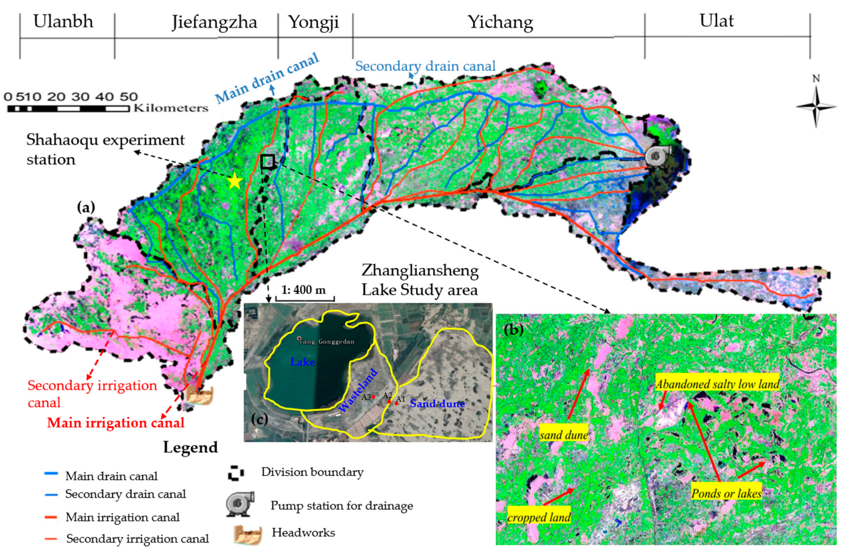
2.1. Study Area

The HID is approximately 50 km long from north to south, and 250 km wide from east to west. Ground slope is 1/5000 to 1/8000 from the west to the east, and 1/4000 to 1/8000 from the south to the north (Figure 1). Hetao is a closed rift basin underlain by Quaternary sediments, mainly lake sediments and alluvial deposits of the Yellow River. The Quaternary aquifer system has two aquifer groups in the basin. The first is composed of two water-bearing strata (Q4 and Q3). Q4 is 6–25 m thick, and the thickness of Q3 ranges from 35 to 240 m. Q4 is mainly constituted of sandy loam materials, while the deposit properties for Q3 consist of fine–medium, fine, and silt sand with some interclays. The second aquifer group consists of the third water-bearing stratum (Q2). Its upper layer consists of stable muddy clay, which prevents groundwater from vertical flow. The lower layer, composed of sand, has high permeability and is confined [26,27]. The depth of groundwater table varies from 0.5 to 3.0 m during the year [28]. Annual precipitation is about 50–144.2 mm. Rainfall mainly occurs from June to August, which is about 70% of annual precipitation. Mean annual temperature is 7.5 °C. The study area is located in the Zhangliansheng site (40°54′36″ N, 107°15′59″ E), which is east of the Jiefangzha irrigation district (JID) in Hetao. The lake area is about 5.12 × 10⁵ m². The sand dune, wasteland, and lake are adjacent. The elevations of the sand dune, wasteland, and lake are 1036, 1029, and 1028 m, respectively.

2.2. Experiment Design

Groundwater observation wells (Figure 2) were installed at Points A1 (sand dune), A2 (sand dune–wasteland junction), and A3 (wasteland), and their elevations were 1031, 1030, and 1029 m, respectively (Figure 2a). The depth of each observation well was 5 m. Groundwater microsensors (CTD-10, Meter Company, San Francisco, CA, USA) were installed in the three observation wells, which were located at a depth of approximately 3.5 m. Groundwater-level, temperature, and electrical-conductivity (EC) data were recorded at 1 h intervals (Figure 2b). The aquifer boundaries of the three different land types were considered and assumed when the experiment was designed, and the study area was set up. According to the geomorphic characteristics of the three land types in the study area, the areas of sand dune, wasteland, and lake are large, while distance between the three constructed observation wells is relatively short. As shown in Figure 1c, the distance between sand dune (A1) and wasteland–sand dune junction (A2), wasteland–sand dune junction (A2) and wasteland (A3), and wasteland (A3) and lake is 10, 50, and 100 m, respectively. The horizontal widths of sand dune, wasteland, wasteland–sand dune junction, and wasteland–lake junction are longer. The horizontal widths of sand dune, wasteland–sand dune junction, wasteland, and wasteland–lake junction are about 1600, 700, 1200, and 1500 m, respectively (determined by Google Earth). Therefore, the boundaries of the sand dune, wasteland, and lake are approximately straight and parallel to each other. We could assume that groundwater only flows through the aquifer boundaries of the three land types. Soil sensors (5TE, Meter Company) were installed at Sites A1–A3, which were embedded in 20, 40, 60, 80, and 100 cm soil layers, respectively (Figure 2c). Soil water content, temperature, and EC data were recorded at 1 h intervals by an EM50 data logger (Meter Company). During the crop-growth period, lake-water samples were collected at 20 day intervals. EC lake values were measured using a conductivity meter (DDS-307A type, Shanghai Youke Instrument Company, Shanghai, China). Meteorological data were collected by an automatic weather station (Davis Instruments, Hayward, CA, USA), which was located at the Shahaoqu experiment station. Distance between Shahaoqu experiment station and study area is about 28 km.

2.3. Test Items

2.3.1. Soil Physical Properties of Study Area

Soil samples at Sites A1–A3 were collected from each soil layer (0–20, 20–40, 40–60, 60–80, 80–100, 100–120, 120–160, and 160–200 cm). A sample from each soil layer was collected in triplicate. Bulk density and saturated soil water content were measured on undisturbed soil samples (100 cm³), collected from the different layers at Sites A1–A3. Saturated hydraulic conductivity was also measured in situ using a Guelph permeameter (2800K1, Santa Barbara, CA, USA). A dry particle sizer (Helos and Rodos, Germany New Partec, Dresden, Germany) was used to determine soil particle size. van Genuchten parameters were estimated on the basis of bulk density; percentages of sand, silt, and clay values; and soil water-retention data using Rosetta pedotransfer functions. Soil components in the 0–200 cm soil layer at Sites A1–A3 consisted of 0.518% clay, 7.494% silt, and 91.691% sand; 3.16% clay, 45.28% silt, and 51.56% sand; and 5.612% clay, 80.064% silt, and 14.324% sand, respectively. Soil bulk densities at Sites A1–A3 were 1.762, 1.66, and 1.678 g cm⁻³, respectively. Saturated hydraulic conductivities of the soil at Sites A1–A3 were 257.59, 22.56, and 18.34 cm d⁻¹. Soil water contents at saturation and residual varied from 0.308 to 0.369 cm³ cm⁻³ and from 0.027 to 0.043 cm³ cm⁻³. Empirical shape parameters α and n in soil water-retention function varied from 0.0127 to 0.0385, and from 1.132 to 2.825 (

Table 1. Fundamental physical properties and parameters of van Genuchten hydraulic model.

Sample	Soil Layer (cm)	Soil Physical Properties					van Genuchten Parameters
		<0.02 mm (%)	0.02–0.5 mm (%)	>0.5 mm (%)	Bulk Density (g cm−3)	Saturated Hydraulic Conductivity (cm d−1)	θr (cm3·cm−3)	θs (cm3·cm−3)	α (cm−1)	n
A1	200	0.518	7.494	91.691	1.762	257.59	0.043	0.308	0.0385	2.825
A2	200	3.16	45.28	51.56	1.66	22.56	0.027	0.309	0.0341	1.132
A3	200	5.612	80.064	14.324	1.678	18.34	0.031	0.369	0.0127	1.853

).

2.3.2. Soil Data

Due to the collapse of the sand dune in 2018, the 5TE sensors and EM50 data logger at Site A1 were damaged. In order to ensure data continuity, soil samples of the 1 m soil layer were collected at 20 day intervals from 8 April to 1 October, and there were 5 sampling layers (0–20, 20–40, 40–60, 60–80, and 80–100 cm). Soil water content at Site A1 was measured by the drying method, and the EC value of the soil extract solution with a soil/water ratio of 1:5 was determined by a conductivity meter (DDS-307A). Automatic sensors were used to monitor soil water content and EC at Sites A2 and A3.

2.3.3. Water-Sample Data

EC values of the lake varied from 2.1 to 3.5 dS m⁻¹ (

Table 2. Variance of lake electrical-conductivity (EC) values (dS m⁻¹).

Year	10 April	30 April	20 May	10 June	30 June	20 July	10 August	30 August	20 September	1 October
2017	2.30	2.50	3.19	2.70	2.80	3.50	2.20	2.20	2.30	2.50
2018	2.10	2.54	3.40	2.57	2.72	3.33	3.04	3.21	3.13	3.22

); which were affected by groundwater [14].

2.3.4. Meteorological Data

As shown in Figure 3, the temperature curve showed seasonal fluctuation in 2017 and 2018. Minimal temperatures in 2017 and 2018 were −12 and −19 °C, respectively; maximal temperature in both years was 28 °C. Rainfall mainly occurred from June to September. Maximal daily precipitation was 10.5 mm on 20 September 2017 and 17.5 mm on 23 August 2018.

2.4. Study Method

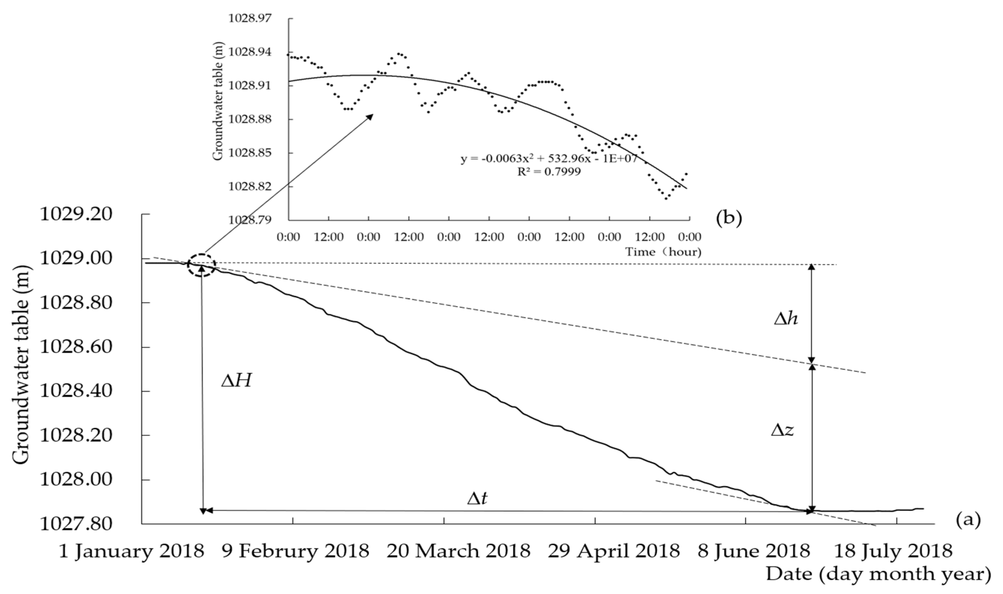
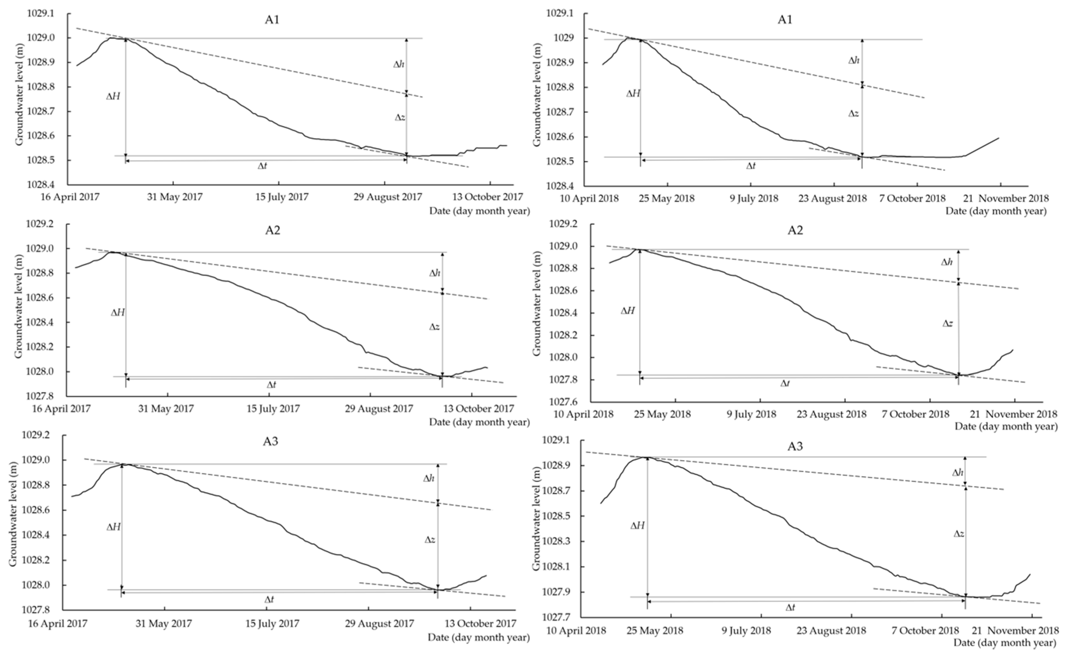
2.4.1. Water-Table-Fluctuation Method

Wang et al. [30] indicated that groundwater-level fluctuations were affected by seasonal trends, daily fluctuations, and residuals in arid regions. The WTF method is mainly based on analysis of seasonal trends in groundwater-table hydrographs H (t), which is usually employed to quantify groundwater recharge/discharge rate [31,32,33,34]. Weeks et al. [35], and Healy et al. [36] suggested that the decision to use the WTF method to estimate ET_g in arid and semiarid areas was mainly based on the following assumptions: (1) seasonal declines in groundwater level, which were mainly affected by ET_g, were relatively stable during the growing season; (2) during the whole growth period, there was no change in lateral flow induced by groundwater recharge/discharge rate; (3) the value of the specific yield was representative of the study area. On the basis of the above assumptions, using the Dupuit assumption for groundwater flow, the transient planar-flow model can be written as follows:

$$-\nabla q_{lat}+E{T}_g=S_y\frac{\partial H}{\partial t}$$

(1)

$$q_{lat}=-T{\nabla }_{x,y}H$$

(2)

where Sy is the specific yield, T is the conductivity coefficient of groundwater flow (mm² d⁻¹), $q_{lat}$ is the groundwater lateral flow rate per unit width (mm d⁻¹), and H is the groundwater level (m).

During the growth period, it was assumed that total change in groundwater level ΔH can be divided into two parts (Figure 4), where Δh (x, y, t) was the change in groundwater level caused by groundwater lateral flow (Figure 4). Values of Δz (z, t) were changes in groundwater level induced by seasonal ET_g. Then, by substituting h and z into Equation (1), the following equation can be obtained:

$$-\nabla q_{lat}+E{T}_g=S_y\frac{\partial (h+z)}{\partial t}$$

(3)

According to our assumption, changes in h are not affected by local recharge/discharge condition, and we can treat these changes as being caused by unknown lateral boundary conditions. Therefore, the water-flow equation for h can be written as follows:

$$-\nabla q_{lat}=S_y\frac{\partial (h)}{\partial t}$$

(4)

Thus,

$$E{T}_g=S_y\frac{\partial (z)}{\partial t}$$

(5)

According to Equations (3)–(5), the following formula can be used to calculate the ET_g for seasonal interval Δt:

$$E{T}_g=S_y\frac{\mathsf{\Delta }H-\mathsf{\Delta }h}{\mathsf{\Delta }t}$$

(6)

The application of Equation (6) to the estimation of ET_g is restricted by the correct determination of lateral-flow-induced water-table change rate Δh/Δt, which is assumed to not be related to the evapotranspiration process. Accuracy of the estimated value of Δh/Δt could be confirmed by the identity of Δh/Δt before and after the growing season (Figure 4a). Twenty-four data points and the least-squares method were used to determine the line slope (Figure 4b). We took the period of the lowest water table as the end stage of crop growing (after growing season), and the period of the highest water table as the early stage of crop growing (before growing season). A key factor in the WTF method was to estimate the specific yield, which depended on soil texture, initial water-table depth, and groundwater-level changes [31,37]. In order to evaluate the specific yield, Crosbie et al. [38] established the specific-yield equation on the basis of parameters of the van Genuchten model:

$$S_y=S_{yu}-\frac{S_{yu}}{{\left[1+{\left(\mathsf{\alpha }\left(\frac{Z_i+Z_f}{2}\right)\right)}^n\right]}^{1-\frac{1}{n}}}, S_{yu}={\theta }_s-{\theta }_r$$

(7)

where θ_s is the saturated water content (cm³ cm⁻³), θ_r is the residual water content (cm³ cm⁻³), Z_i is the initial groundwater depth (cm), Z_f is the final groundwater depth (cm), and α and n are the parameters of the van Genuchten model (Table 1).

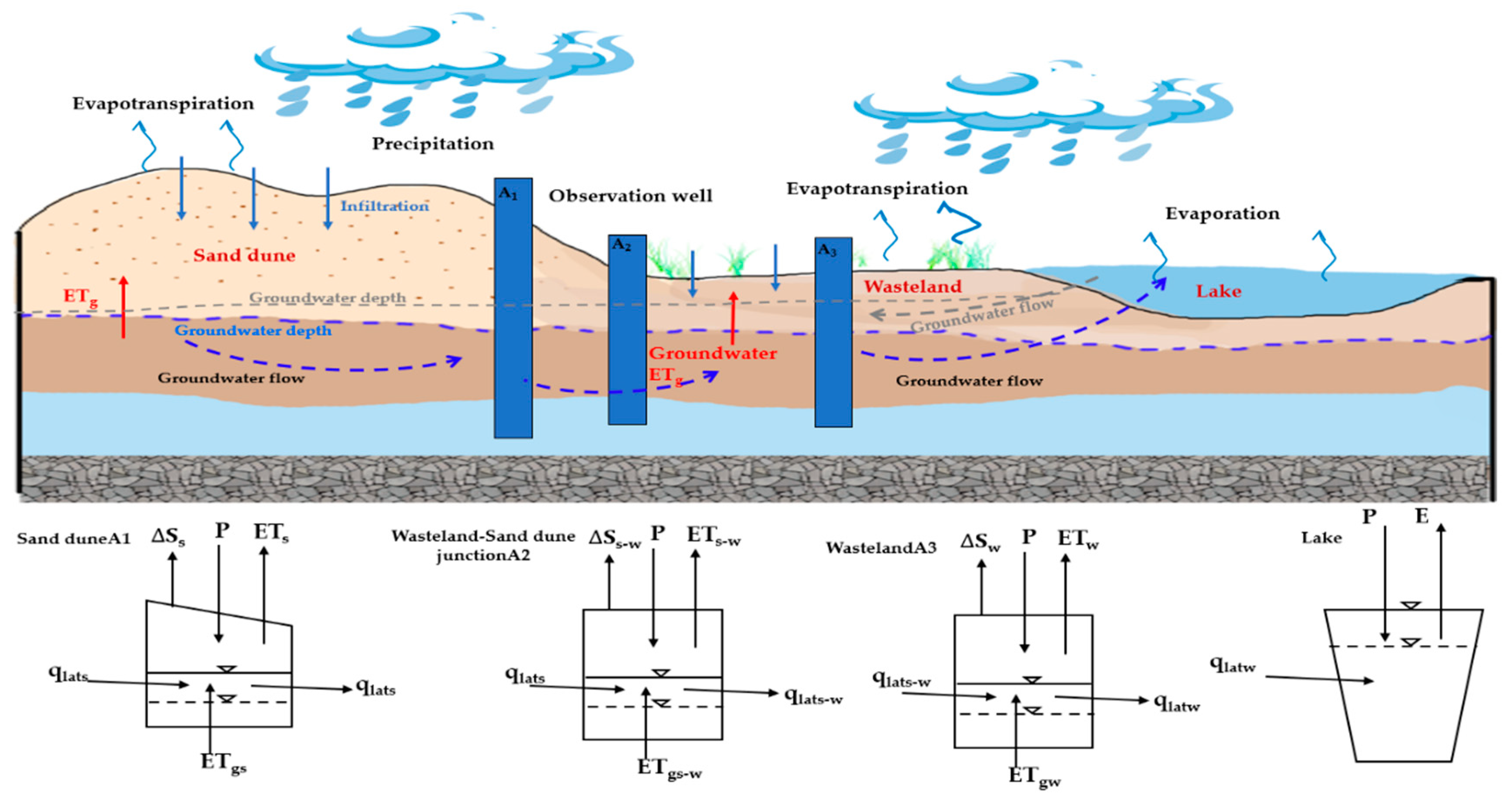
2.4.2. Water-Balance Model

As shown in Figure 5, we assumed that groundwater loss is caused by groundwater evaporation and transpiration. Groundwater evaporation is caused by soil evaporation, and groundwater transpiration is caused by the root water uptake of vegetation. Groundwater loss caused by groundwater evapotranspiration can be defined as the amount of recharge of groundwater to the soil. Therefore, on the basis of the water-balance model, for sand dunes, water inflow has three main resources: precipitation, groundwater recharge, and groundwater lateral inflow; water outflow is mainly through evapotranspiration and groundwater lateral outflow. For the wasteland–sand dune junction, water inflow has three main resources: precipitation, groundwater recharge, and groundwater lateral outflow of sand dune; water outflow is mainly through the evapotranspiration and groundwater lateral outflow of the wasteland–sand dune junction. For the wasteland, water inflow has three main resources: precipitation, groundwater recharge, and groundwater lateral outflow of wasteland–sand dune junction; water outflow is mainly through the evapotranspiration and groundwater lateral outflow of the wasteland. For the lake, water inflow has two main resources: precipitation and groundwater lateral outflow of wasteland; water outflow is mainly through evaporation.

A water-balance model was established for the sand dune–wasteland–lake system (Figure 5). Since the groundwater depth of sand dunes was deep, and there was no vegetation coverage in sand dune (Figure 5), we assumed that groundwater transpiration was not considered, and groundwater loss only was caused by groundwater evaporation (E_gs). Groundwater evaporation (E_gs) was defined as groundwater recharge to sand-dune soil. The water-balance model at Site A1 (sand dune) was established as follows:

$$E{T}_s=P+(E_{gs}+q_{lats}-q_{lats})\times N+\mathsf{\Delta }{S}_s$$

(8)

where ET_S is evapotranspiration of the sand dune (mm); P is precipitation (mm); N is the number of days (d); E_gs is groundwater recharge to sand-dune soil (mm d⁻¹), and positive values indicate the amount of groundwater recharge to soil; ΔS_s is the amount of storage consumption of the unsaturated zone and sand-dune groundwater (mm); and $q_{lats}$ is the lateral flow rate of sand-dune groundwater (mm d⁻¹).

Since the groundwater depths of the wasteland and wasteland–sand dune junction were lower than that of the sand dune, and there was vegetation in the wasteland and wasteland–sand dune junction (Figure 5), we assumed that groundwater loss was caused by groundwater evaporation and transpiration. We defined the groundwater evapotranspiration of the wasteland (ET_gw) and wasteland–sand dune junction (ET_gs–w) as groundwater recharge to the soil of the wasteland and wasteland–sand dune junction, respectively.

The water-balance model at Site A2 (wasteland–sand dune junction) was as follows:

$$E{T}_{s-w}=P+(E{T}_{gs-w}+q_{lats}-q_{lats-w})N+\mathsf{\Delta }{S}_{s-w}$$

(9)

where ET_s–w is the evapotranspiration of the wasteland–sand dune junction (mm); ET_gs–w is the groundwater recharge to the soil of the wasteland–sand dune junction (mm d⁻¹), and positive values indicate the amount of groundwater recharge to soil; ΔS_s–w is the amount of storage consumption of the unsaturated zone and the groundwater of the wasteland–sand dune junction (mm); $q_{lats}$ is the lateral flow rate of sand-dune groundwater to the wasteland–sand dunes junction (mm d⁻¹); and $q_{lats-w}$ is the lateral flow rate of wasteland–sand dune junction groundwater to the wasteland (mm d⁻¹).

The water-balance model at Site A3 (wasteland) was as follows:

$$E{T}_w=P+(E{T}_{gw}+q_{lats-w}-q_{latw})N+\mathsf{\Delta }{S}_w$$

(10)

where ET_w is the evapotranspiration of the wasteland (mm); ET_gw is groundwater recharge to the soil of the wasteland (mm d⁻¹), and positive values indicate the amount of recharge of groundwater to soil; ΔS_w is the amount of storage consumption of the unsaturated zone and wasteland groundwater (mm); and $q_{latw}$ is the lateral flow rate of wasteland groundwater to the lake (mm d⁻¹).

The water-balance model of the lake was established as follows:

$$\mathsf{\Delta }W=P+q_{latw}\times N-0.59E_0$$

(11)

where ΔW is lake water loss (mm), where positive values indicate a decrease in lake-water amount; $E_0$ is the evaporation of the $\varphi 20$ evaporating dish. The conversion factor of the $\varphi 20$ evaporation dish is 0.59 in the study area [14]. The water-balance model of the lake did not consider the indirect recharge of irrigation.

$$\mathsf{\Delta }S=S_y\cdot \mathsf{\Delta }H$$

(12)

where $\mathsf{\Delta }S$ is the amount of storage consumption (mm) of the unsaturated zone and groundwater, and a positive value indicates the amount of storage consumption; ΔH = H_i − H_f; H_i is the initial water table (m); and H_f is the final water table (m).

2.4.3. Groundwater Salt-Transport Model in Sand Dune–Wasteland–Lake System

The conversion formula of groundwater EC and groundwater total dissolved solids (TDS) is [14]

$$TDS=0.69E{C}_w$$

(13)

where TDS is groundwater total dissolved solids (g L⁻¹) and EC_w is groundwater electrical conductivity (dS m⁻¹).

Horizontal Groundwater Salt-Transport Model

Horizontal salt transport from Site A1 (sand dune) to Site A2 (wasteland–sand dune junction):

$$L_{s\to s-w}=q_{la{t}_s}\times N\times TD{S}_s\times 10$$

(14)

where L_s→s–w is the horizontal salt transport from A1(sand dune) to A2 (wasteland–sand dune junction) (kg hm⁻²). TDS_S is the sand-dune groundwater total dissolved solids (g L⁻¹).

Horizontal salt transport from Site A2 (wasteland–sand dune junction) to Site A3 (wasteland):

$$L_{s-w\to w}=q_{la{t}_{s-w}}\times N\times TD{S}_{s-w}\times 10$$

(15)

where L_s–w→w is horizontal salt transport from Site A2 (wasteland–sand dune junction) to Site A3 (wasteland) (kg hm⁻²). TDS_S–w is the wasteland–sand dune junction groundwater total dissolved solids (g L⁻¹).

Horizontal salt transport from A3 (wasteland) to the lake:

$$L_{w\to l}=q_{la{t}_w}\times N\times TD{S}_w\times 10$$

(16)

where L_w→l is horizontal salt transport from Site A3 (wasteland) to the lake (kg hm⁻²). TDS_w is the wasteland groundwater total dissolved solids (g L⁻¹).

Estimation of groundwater salt accumulation at Site A2 (wasteland–sand dune junction):

$$\mathsf{\Delta }{L}_{s-w}=L_{s\to s-w}-L_{s-w\to w}$$

(17)

where ΔL_s→w is groundwater salt accumulation at Site A2 (kg hm⁻²).

Estimation of groundwater salt accumulation at Site A3 (wasteland):

$$\mathsf{\Delta }{L}_w=L_{s-w\to w}-L_{w\to l}$$

(18)

where ΔL_w is groundwater salt accumulation at Site A3 (kg hm⁻²).

Vertical Groundwater Salt-Transport Model

Site A1 (sand dune):

$$S_s=E{T}_{gs}\times N\times TD{S}_s\times 10$$

(19)

where S_s is the vertical salt transport of groundwater at Site A1 (kg hm⁻²).

Site A2 (wasteland–sand dune junction):

$$S_{s-w}=E{T}_{gs-w}\times N\times TD{S}_{s-w}\times 10$$

(20)

where S_s–w is the vertical salt transport of groundwater at Site A2 (kg hm⁻²).

Site A3 (wasteland):

$$S_w=E{T}_{gw}\times N\times TD{S}_w\times 10$$

(21)

where S_w is the vertical salt transport of groundwater at Site A3 (kg hm⁻²).

2.4.4. Soil Salt-Storage Equation

The conversion formula of soil EC and total soil salt content is [39]

$$C=E{C}_{1:5}\times 3.7657-0.2405$$

(22)

where C is total soil salt content (g kg⁻¹) and EC_1:5 is the electrical-conductivity value of the soil extract solution with a soil/water ratio of 1:5.

For soil salt storage, the calculation equation is [40]

$$S=100C{\rho }_{s}l$$

(23)

where S is the soil salt storage (kg hm⁻²), ${\rho }_s$ is bulk density (g cm⁻³), and l is soil-layer depth (cm).

3. Results

3.1. Groundwater Dynamics in Sand Dune–Wasteland–Lake System

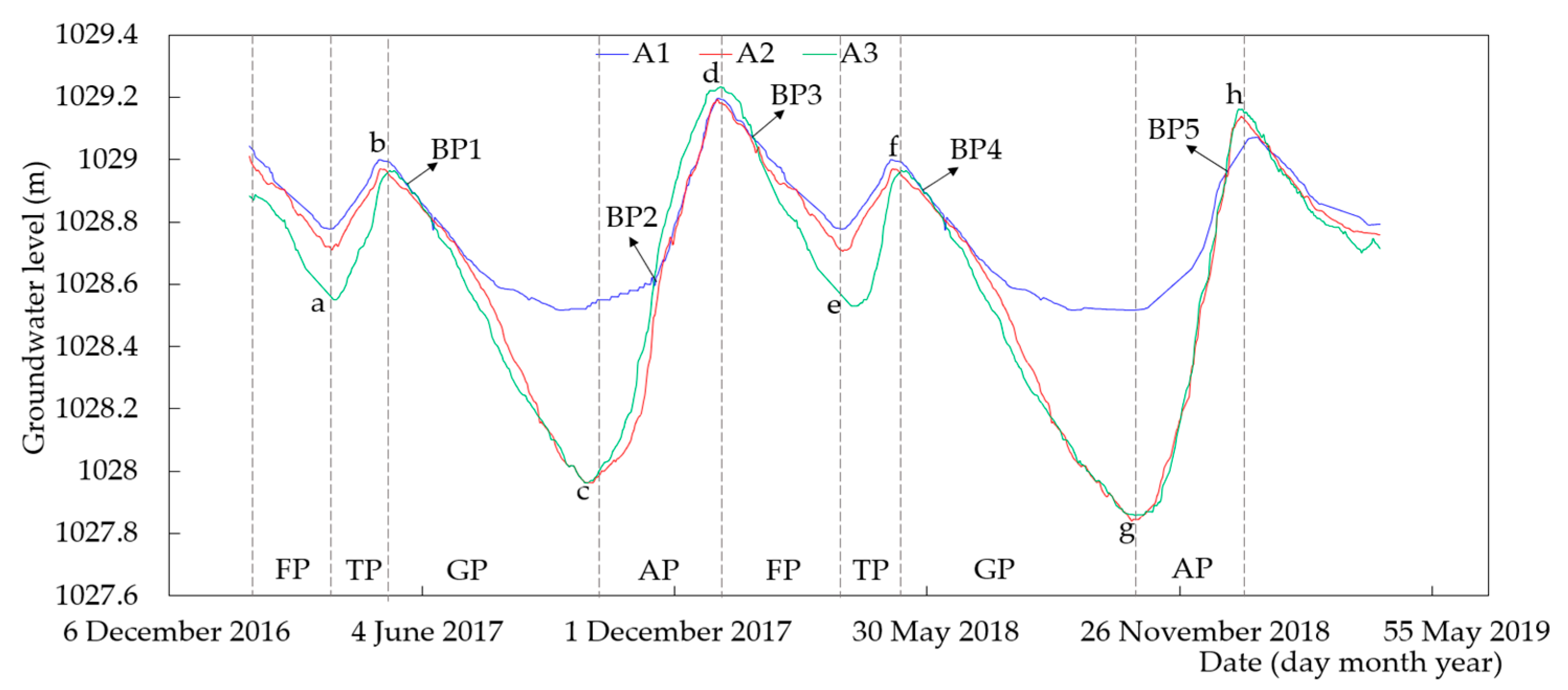
3.1.1. Groundwater-Level Fluctuation in Different Periods

The HID has four periods in the whole year, the freezing (December to March), thawing (April to May), growing (May to October), and autumn-irrigation (October to December) periods, as shown in Figure 6 and

Table 3. Characteristic points of groundwater level in different periods.

Time	Turning Point	Observation Points
		A1 (m)	A2 (m)	A3 (m)
31 March 2017	a	1028.778	1028.714	1028.56
6 May 2017	b	1029	1028.968	1028.93
29 September 2017	c	1028.521	1027.963	1027.963
1 January 2018	d	1029.198	1029.191	1029.228
3 March 2018	e	1028.778	1028.705	1028.56
5 May 2018	f	1029	1028.968	1028.93
27 October 2018	g	1028.517	1027.845	1027.86
8 January 2019	h	1029.73	1029.137	1029.16

. Letters a–h refer to the turning point of groundwater in the different periods.

During the freezing period, the temperature of the frozen soil layer was lower, and the temperature of the shallow groundwater was higher. The frozen soil layer absorbed heat from the shallow groundwater, and the groundwater recharged the frozen soil layer with water vapors, resulting in groundwater-level decline [41]. During the freezing period in 2018, groundwater levels at Sites A1–A3 decreased by 0.42, 0.48, and 0.67 m, respectively (Table 3). During the thawing period, the frozen soil layer gradually melted, and soil water recharged the groundwater. During the thawing period in 2017 and 2018, groundwater levels at Sites A1–A3 increased by 0.22, 0.255, and 0.37 m, respectively (Table 3). During the crop-growth period, air temperature gradually increased, at which time, much water was consumed. The study area did not have irrigation water supplied to it, so soil water could only be recharged by groundwater. During the crop-growth period in 2017 and 2018, groundwater levels at Sites A1–A3 decreased by 0.48, 1.06, and 1.02 m, respectively (Table 3). In the autumn-irrigation period, an amount of autumn-irrigation water was diverted from the Yellow River to the HID to leach salt from the cultivated land and drain salt out of the irrigation area. Excess autumn-irrigation water was drained into the lake; therefore, the lake level increased. The groundwater of the wasteland and sand dunes is recharged through the lake. Groundwater levels at Sites A1–A3 increased by 0.63, 1.26, and 1.28 m, respectively, during the autumn-irrigation period in 2017 and 2018 (Table 3). The sand dune–wasteland–lake system was in a state of water deficiency during the growth period, whereas it was in a state of water surplus in the autumn-irrigation period. The sand dune–wasteland–lake system can maintain water in balance during the whole year.

3.1.2. Groundwater Transport Direction

As shown in Figure 6, and Table 3 and

Table 4. Balance points of groundwater level between sand dune and wasteland in different periods.

Balance Point	Date	Groundwater Level (m)
BP1	23 May 2017	1028.927
BP2	16 November 2017	1028.6
BP3	26 January 2018	1029.07
BP4	28 May 2018	1028.894
BP5	23 December 2018	1028.94

, from BP1 (H:1028.927 m; 23 May 2017) to turning point c (29 September), groundwater levels at Sites A1 and A3 both decreased, and groundwater level at Site A1 was higher than that of Site A3. Lake evaporation was high. A hydraulic gradient was observed in the sand dune–wasteland–lake system, and the transport direction of the groundwater was from the sand dune to the lake. At turning point c–BP2 (H: 1028.6 m; 16 November 2017), groundwater levels at Sites A1–A3 increased, and groundwater levels at Sites A1 and A2 increased faster than that of A3; at BP2–BP3 (H: 1029.07 m; 26 January 2018), groundwater level at Site A3 was higher than that of A1. During the autumn-irrigation and early freezing periods, the transport direction of groundwater was from the lake to the sand dune. At BP3–BP4 (H: 1028.894 m; 28 May 2018), groundwater level at Site A1 was higher than that of Site A3. During the freezing period, the wasteland groundwater recharged the frozen soil layer with a profusion of water, and the groundwater levels of the wasteland significantly declined. In the middle and late freezing, and thawing periods, the transport direction of the groundwater was from the sand dune to the lake. At BP4–BP5 (H: 1028.94 m; 23 December 2018), the transport direction of groundwater was consistent with that of BP1–BP2.

In summary, during the growth period, the transport direction of groundwater was from the sand dune to the lake. During the autumn-irrigation and early freezing periods, the transport direction of groundwater was from the lake to the sand dune. During the middle and late freezing, and thawing periods, the transport direction of groundwater was from the sand dune to the lake.

3.2. Water-Balance Estimation

3.2.1. Estimation of Specific Yield and Storage Changes of Unsaturated Zone and Groundwater

The growth periods (b–c, f–g) in 2017 and 2018 were selected as the study period. Specific yield S_y was determined using Equation (7), and ΔS was determined using Equation (12). As shown in

Table 5. Statistical table of water-balance parameters in the growth period.

Date	Observation Point	ΔH (m)	Δh (m)	Δz (m)	Δt (d)	Sy	−∇qlat (mm d−1)	ETg (mm d−1)	ΔS (mm)	P (mm)	ET (mm)
b–c	A1	0.48	0.22	0.26	126.00	0.26	0.45	0.54	124.80	53.4	246.24
	A2	1.01	0.31	0.70	146.00	0.06	0.13	0.29	60.60	53.4	203.68
	A3	0.97	0.27	0.70	146.00	0.07	0.12	0.31	63.05	53.4	163
f–g	A1	0.48	0.19	0.29	124.00	0.26	0.40	0.61	124.80	113.4	313.6
	A2	1.12	0.28	0.84	175.00	0.06	0.10	0.29	67.20	113.4	283.92
	A3	1.07	0.19	0.88	176.00	0.07	0.07	0.33	69.55	113.4	244.7

, S_y values at Sites A1–A3 were 0.26, 0.06, 0.07, respectively. Zhang et al. [42] found that S_y values in silty loam soil varied from 0.04 to 0.06. Cai et al. [43] reported that S_y values in sand soil were 0.15, 0.26, 0.263, and 0.274. Comparing our results with those of the aforementioned studies, the values of S_y that we obtained are representative of study area.

During the entire growth period in 2017 and 2018, the average ΔS value at Sites A1–A3 decreased by 124.8, 63.9, and 66.3 mm, respectively. Sand-dune water consumption was 1.95 times that of the wasteland–sand dune junction, and 1.88 times that of the wasteland. Sand-dune water consumption was about 60 mm more than that at the wasteland–sand dune junction and wasteland because the transport direction of groundwater was from sand dunes to the lake during the growth period. The values of S_y in the sand dune were large, and groundwater lateral flow was faster. ΔS at Sites A2 and A3 was similar, which was due to the similar soil texture and specific yield. During the growing period, sand dunes, wasteland, and the lake were in a state of water consumption.

3.2.2. Estimation of ET_g and −∇q_lat

Growth periods (b–c, f–g) in 2017 and 2018 were selected as the study period to analyze the seasonal changes of groundwater. According to the WTF method, Δh and Δz at Sites A1–A3 were determined. As shown in Table 5 and Figure 7, differences in Δh and Δz at Sites A1–A3 were small. On the basis of Equations (3) and (4), groundwater lateral flow was estimated. As shown in Table 5, values of –Δq_lat at Sites A1–A3 were 0.45, 0.13, and 0.12 mm d⁻¹ for study period b–c, and 0.40, 0.10, and 0.07 mm d⁻¹ for study period f–g, respectively. Differences in –Δq_lat value at Sites A1–A3 were 0.05, 0.03, and 0.05 mm d⁻¹, respectively. Differences in –Δq_lat value were small, which were acceptable and stable for the study area.

On the basis of Equations (5) and (6), ET_g was estimated. As shown in Table 5, ET_g values at Sites A1–A3 in the two growth periods (b–c, f–g) were 0.54, 0.29, and 0.31 mm d⁻¹ for growth period b–c, and 0.61, 0.29, and 0.33 mm d⁻¹ for growth period f–g, respectively. Differences in ET_g values at Sites A1–A3 were 0.07, 0, and 0.02 mm d⁻¹, respectively. Differences in ET_g values were small, which were acceptable and stable for the study area.

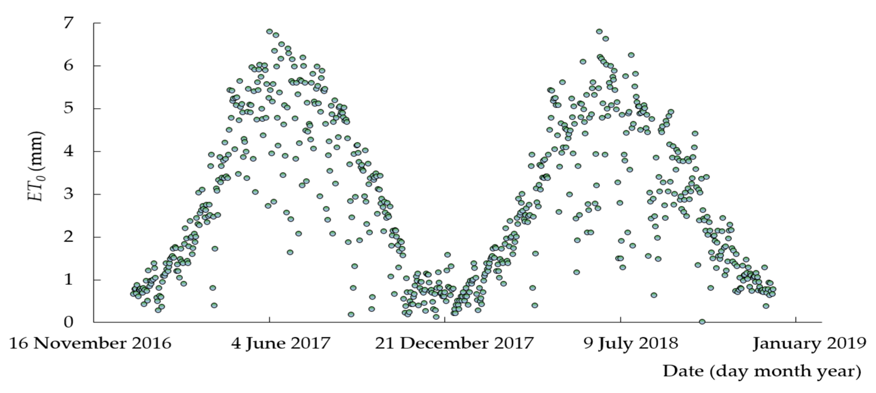
3.2.3. Evapotranspiration Estimations

Growth periods (b–c, f–g) in 2017 and 2018 were selected as the study period to calculate evapotranspiration in the sand dune–wasteland–lake system on the basis of Equations (8)–(10). ET values at Sites A1–A3 were 246.24, 203.68, and 163 mm for growth period b–c, and 313.6, 283.92, and 244.7 mm for growth period f–g, respectively. ET values at Sites A1–A3 in 2018 were, respectively, 67.36, 80.24, and 81.7 mm higher than those in 2017. As shown in Table 3 and Figure 5, autumn irrigation in 2018 was 28 d later than that of 2017, and air temperature was higher in 2018; therefore, evapotranspiration in 2018 was higher than that in 2017. As shown in Figure 8, ET₀ values during the growth period in 2017 and 2018 were 656 and 665 mm, respectively. Average ET values at Sites A1–A3 during the two growth periods (b–c, f–g) were 42%, 37%, and 31% of ET₀. There was no irrigation supply in the study area, and water shortage was serious. The ET of the study area was 31%–42% of ET₀.

On the basis of Equation (11), water loss of the lake was 869.05 and 761.25 mm during the growth period in 2017 and 2018, respectively (

Table 6. Lake water loss.

Year	Precipitation (mm)	Transport Recharge (mm)	Water Evaporation (mm)	ΔW (mm)
2017	53.4	17.55	940	−869.05
2018	113.4	12.35	887	−761.25

). Water shortage in 2017 was 107.8 mm more than that in 2018 since precipitation was less and lake evaporation was high in 2017. If there was no water supply, the lake would face the risk of drying up.

3.3. Salt-Balance Calculation

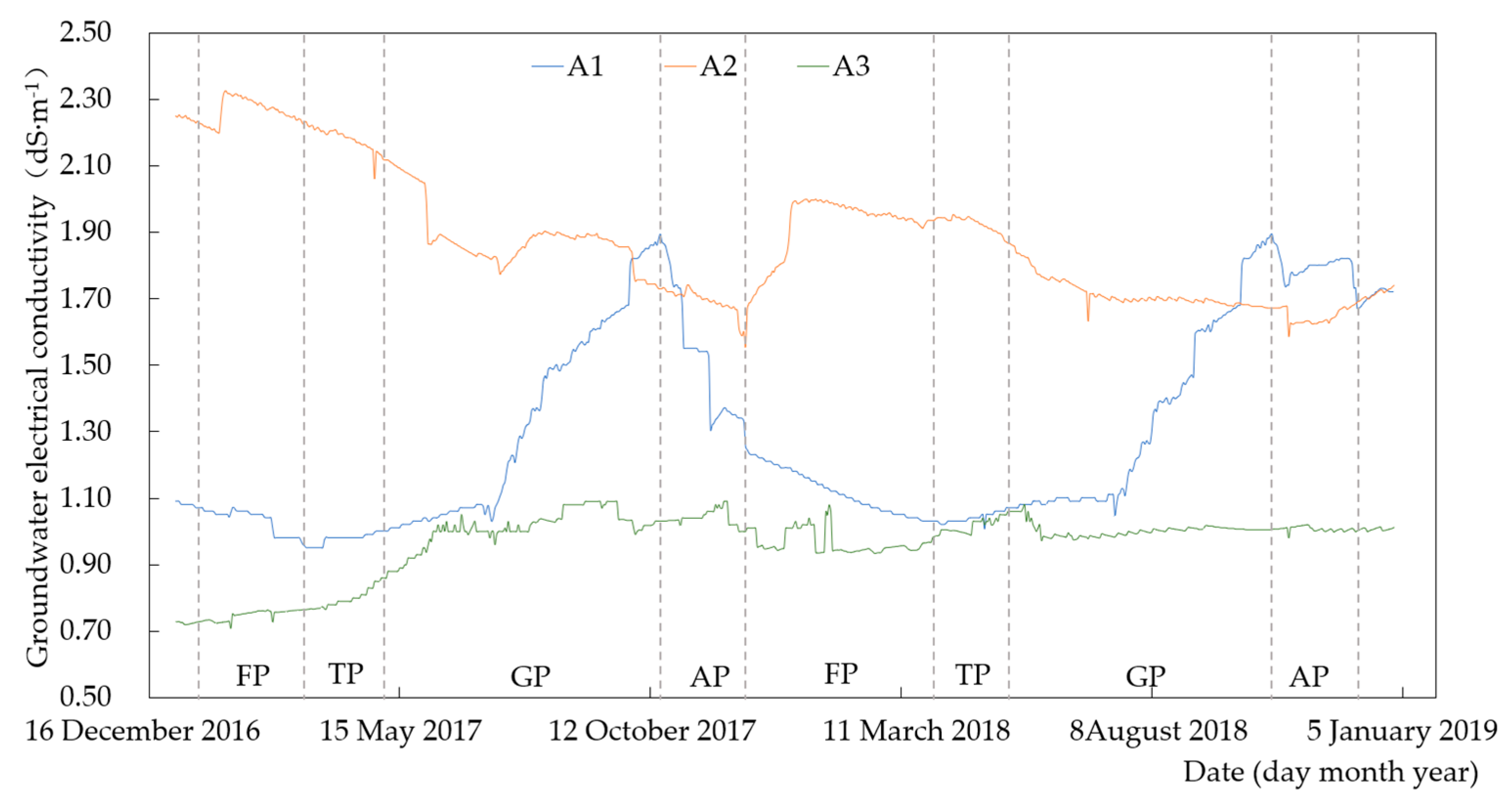
3.3.1. Groundwater EC Dynamics in 2017 and 2018

During the growth period, the transport direction of the groundwater was from the sand dune to the lake. Groundwater lateral flow was large, and the top of the sand-dune groundwater supplied Site A1, so groundwater EC varied from 1.05 to 1.92 dS m⁻¹. As shown in Figure 9, groundwater EC values at Site A1 were lower than those of Site A2. During the transport process of groundwater, groundwater EC at Site A2 was diluted, and groundwater EC values varied from 2.1 to 1.7 dS m⁻¹. Groundwater EC of the wasteland increased slightly, varying from 0.85 to 1.05 dS m⁻¹. During the autumn-irrigation period, the transport direction of the groundwater was from the lake to the sand dune. Groundwater EC at Site A3 was lower, so groundwater EC at Sites A1 and A2 varied from 1.85 to 1.23 dS m⁻¹ and from 1.7 to 1.52 dS m⁻¹, respectively. In the middle and late freezing, and thawing periods, the transport direction of the groundwater was from the sand dune to the lake. Since groundwater EC at Site A1 was lower, during the transport process of groundwater, groundwater EC at Site A2 was diluted. Groundwater EC at Site A2 varied from 2.0 to 1.85 dS m⁻¹. Since groundwater EC at Site A2 was larger than that of Site A3, groundwater EC of the wasteland increased slightly, varying from 0.91 to 1.08 dS m⁻¹.

3.3.2. Estimation of Vertical Salt Transport of Groundwater

Growth periods (b–c, f–g) in 2017 and 2018 were selected as the study period to calculate the vertical salt transport of groundwater at Sites A1–A3 on the basis of Equations (19)–(21). As shown in

Table 7. Vertical salt transport of groundwater.

Date	Observation Point	N (d)	ETg (mm d−1)	TDS (g L−1)	Salinity (kg hm−2)
b–c	A1	126	0.54	0.88	598.75
	A2	146	0.29	1.31	554.65
	A3	146	0.31	0.70	316.82
f–g	A1	124	0.61	0.93	703.45
	A2	175	0.29	1.19	603.93
	A3	176	0.33	0.69	400.75

, the average values of the vertical salt transport of groundwater at Sites A1–A3 during the two study periods (b–c, f–g) were 651.10, 579.29, and 358.79 kg hm⁻², respectively. The vertical salt transport of groundwater at the sand dunes site was 1.13 times that at the wasteland–sand dune junction site and 1.82 times that at the wasteland site. The vertical salt transport of groundwater at Site A1 was 71.81 and 292.32 kg hm⁻² more than those of Sites A2 and A3, respectively, and the vertical salt transport of groundwater at Site A2 was 220.50 kg hm⁻² more than that of Site A3. Due to the values of S_y being large, the value of ET_g at Site A1 was 1.8 times that at Sites A2 and A3. Groundwater TDS at Site A2 was 1.38 and 1.80 times that at Sites A1 and A3, respectively.

3.3.3. Estimation of Horizontal Salt Transport of Groundwater

Growth periods (b–c, f–g) in 2017 and 2018 were selected as the study period to calculate the horizontal salt transport of groundwater at Sites A1–A3, and estimate groundwater salt accumulation at Sites A2 and A3 on the basis of Equations (14)–(18). As shown in

Table 8. Horizontal salt transport of groundwater.

Date	Transport Direction	N (d)	−∇qlat (mm d−1)		TDS (g L−1)	L (kg hm−2)		ΔL (kg hm−2)
b–c	A1→A2	126	qlats	0.45	0.88	Ls→s–w	498.96	ΔLs–w	250.32
	A2→A3	146	qlats–w	0.13	1.31	Ls–w→w	248.64			ΔLw	126.00
	A3→Lake	146	qlatw	0.12	0.70	Lw→l	122.64
f–g	A1→A2	124	qlats	0.40	0.93	Ls→s–w	461.28	ΔLs–w	253.03
	A2→A3	175	qlats–w	0.10	1.19	Ls–w→w	208.25			ΔLw	123.24
	A3→Lake	176	qlatw	0.07	0.69	Lw→l	85.01

, the average value of the horizontal salt transport of groundwater from Site A1 to Site A2 was 480.12 kg hm⁻²; from Site A2 to Site A3, it was 228.44 kg hm⁻²; and from Site A3 to the lake, it was 103.82 kg hm⁻². Of sand-dune groundwater salt, 54% was accumulated in the groundwater of the wasteland–sand dune junction. Of the groundwater salt of the wasteland–sand dune junction, 53% was accumulated in wasteland groundwater, and the remaining 47% was accumulated in the lake. The average values of estimated groundwater salt accumulation at Sites A2 and A3 were 251.68 and 124.62 kg hm⁻², respectively. Groundwater in the sand dune–wasteland–lake system was in a state of salt accumulation during the growing period.

3.3.4. Estimation of Soil Salt Storage

On the basis of Equations (22) and (23), the salt storage of the 1 m soil layer at Sites A1–A3 was estimated for different periods. As shown in

Table 9. Salt-storage changes at Site A1 in different periods (kg hm⁻²).

Soil Layers (cm)	10 April	30 April	20 May	10 June	30 June	20 July	10 August	30 August	20 September	1 October
0–20	678	678	678	744	877	877	1075	1009	1142	1333
20–40	2003	2136	2401	2467	2600	2666	3064	3594	4389	4522
40–60	3594	3925	3859	4190	4190	4323	4456	4721	5251	5450
60–80	3992	4124	4787	5649	6643	7438	8432	9426	9559	8764
80–100	5383	5781	5781	7107	8432	9360	9625	11,746	13,734	15,723
Sum	15,650	16,644	17,506	20,157	22,742	24,664	26,652	30,496	34,075	35,790

Note: values in Table 9, Table 10 and Table 11 are average values of salt storage in 2017 and 2018.

, the total amount of salt accumulated at the 1 m soil layer of the sand dune was 20,140 kg hm⁻² from 10 April to 1 October, and the salt accumulation rate was 56%.

As shown in

Table 10. Salt-storage changes at Site A2 in different periods (kg hm⁻²).

Soil Layers (cm)	10 April	30 April	20 May	10 June	30 June	20 July	10 August	30 August	20 September	1 October
0–20	1975	1796	1647	1475	1143	1197	1280	1327	1202	2629
20–40	26,537	27,706	28,553	31,895	33,046	33,832	32,866	35,807	35,684	35,663
40–60	1014	1264	1264	1236	1389	1606	1264	1702	1639	2077
60–80	3077	3577	4713	4367	3825	4640	4890	5828	6015	6109
80–100	12,501	12,514	13,063	14,689	17,353	19,348	19,114	21,672	21,955	22,325
Sum	45,105	46,857	49,241	53,662	56,756	60,623	59,414	66,335	66,496	68,804

, the total amount of salt accumulated at the 1 m soil layer of the wasteland–sand dune junction was 23,699 kg hm⁻² from 10 April to 1 October, and the salt accumulation rate was 34%.

As shown in

Table 11. Salt-storage changes at Site A3 in different periods (kg hm⁻²).

Soil Layers (cm)	10 April	30 April	20 May	10 June	30 June	20 July	10 August	30 August	20 September	1 October
0–20	9573	11,774	12,403	13,032	14,290	16,805	17,434	17,811	18,063	18,503
20–40	8064	10,076	9636	11,714	13,035	15,579	14,570	16,554	17,413	17,308
40–60	17,874	18,928	20,010	19,761	19,950	21,836	23,849	24,037	24,729	24,729
60–80	19,258	20,410	20,874	20,975	21,333	21,459	21,689	22,562	22,591	22,842
80–100	24,079	21,231	18,705	20,712	20,594	19,698	18,548	19,918	19,200	19,950
Sum	78,848	82,419	81,628	86,194	89,201	95,377	96,090	100,882	101,996	103,332

, the total amount of salt accumulated at the 1 m soil layer of the wasteland was 24,484 kg hm⁻² from 10 April to 1 October, and the salt accumulation rate was 24%.

In summary, the study area was in a state of salt accumulation during the growing period. The salt storage of the 1 m soil layer of the sand dune was 85% that of the wasteland–sand dune junction and 82% that of the wasteland. The total amount of salt accumulated at the 1 m soil layer of the wasteland was 4344 kg hm⁻², which was 785 kg hm⁻² more than that of the sand dune and the wasteland–sand dune junction.

4. Discussion

We studied groundwater dynamics in a sand dune–wasteland–lake system, and revealed the transport direction of groundwater in different periods. On the basis of the water–salt balance model, water and salt in a sand dune–wasteland–lake system were estimated. Results showed that groundwater fluctuation had periodicity, which was a typical seasonal-dynamics pattern. Krogulec [44] evaluated the risk of groundwater drought in groundwater-dependent ecosystems in the central part of the Vistula river valley, Poland, and showed that groundwater-level changes over the study period can be classified as exhibiting hydroperiods of the periodic type, with a typical seasonal-level fluctuation pattern. The results of this paper are similar to those of Krogulec et al. (2018). Ceng [23] proposed that the groundwater of cultivated land recharged sand dunes and lakes during the irrigation period, while sand-dune groundwater recharges wasteland and lakes in nonirrigation periods. Results showed that the groundwater transport direction in the sand dune–wasteland–lake system changed in different periods (freezing, thawing, growth, and autumn-irrigation periods), and the dynamics of groundwater EC was affected by the groundwater transport path (Figure 9). The average value of the horizontal salt transport of groundwater from sand dune to wasteland–sand dune junction was 480.12 kg hm⁻², 228.44 kg hm⁻² from wasteland–sand dune junction to wasteland, and 103.82 kg hm⁻² from wasteland to lake (Table 8). Wang [14] showed that the average value of the salt transport of groundwater from cultivated land to wasteland was 3232 kg hm⁻², and 3134 kg hm⁻² from wasteland to lake. Since the sand dune–wasteland–lake system is not affected by irrigation, the groundwater hydraulic gradient is small, and −Δq_lat values at Sites A1–A3 were 0.45, 0.13, and 0.12 mm d⁻¹ for study period b–c, and 0.40, 0.10, and 0.07 mm d⁻¹ for study period f–g, respectively (Table 5). The amount of groundwater transport was less. Wang [14] showed that lake water loss was 631–706 mm. Results showed that lake water loss was 761.25–869.05 mm during the growth period (Table 6), which was 140–163 mm more than that reported by Wang et al. (2019) because the indirect recharges of irrigation were not considered. Wang [16] showed that the estimated ET_g rate ranged from 0.63 to 0.73 mm d⁻¹, with an average of 0.67 mm d⁻¹. Results showed that average values of ET_g at Site A1 in the growth periods were 0.58 (Table 5). Si [45] showed that the total evapotranspiration of Tamarix ramosissima was approximately 248 mm with an evapotranspiration rate of 1.6 mm d⁻¹. Results showed the ET values at Sites A2 and A3 ranged from 203.68 to 283.92 mm, and from 163 to 244.7 mm during the growth period, which is similar to the results of Si et al. (2005), which are representative of the study area. Krogulec [46] pointed out that hydrogeological studies need a more interdisciplinary approach and the integration of various fields of natural sciences. Ren et al. [19], Yue et al. [20], and Wang et al. [14] studied the water- and salt-transport process for an irrigation and drainage unit, nonagricultural–agricultural–water areas, and a cultivated land–wasteland–lake system, respectively, by constructing water and salt balance models. In this study, three methods, i.e., water-table fluctuation (WTF), soil hydrodynamics, and solute dynamics, were combined to build a water and salt balance model to reveal the relationship of water and salt transport in a sand dune–wasteland–lake system, and quantitatively estimated water consumption and the amount of salt transportation. There are also some aspects that were not considered. In this paper, hydrology models, i.e., HYDRUS, SWAP, MODFLOW, and WSMS_Q3D, were not considered to simulate the water and salt transport process. Most traditional regional modeling may oversimplify the effects of fragmented land covers on hydrological processes [47]. Therefore, just like a sand dune–wasteland–lake system, the simulation accuracy of a regional hydrological model is limited. Therefore, it is necessary to expand the study area in the future, and build a large-scale hydrological groundwater monitoring network to study the water and salt transport process.

5. Conclusions

(1)

The groundwater transport direction in the sand dune–wasteland–lake system changed during different periods. The dynamics of groundwater EC were affected by the groundwater transport path.

(2)

During the growth period in 2017 and 2018, sand-dune water consumption was 1.95 times that of the wasteland–sand dune junction and 1.88 times that of the wasteland. Average ET values of the sand dunes, wasteland–sand dune junction, and wasteland were 42%, 37%, and 31%, respectively, of the ET₀. Lake water loss was 761.25–869.05 mm. If there was no water supply, the lake would dry up.

(3)

During the growth period, the vertical salt transport of groundwater at the sand-dune site was 1.13 times that at the wasteland–sand dune junction site and 1.82 times that at the wasteland site. Of sand-dune groundwater salt, 54% was accumulated in the groundwater of the wasteland–sand dune junction. Of the groundwater salt of the wasteland–sand dune junction, 53% was accumulated in wasteland groundwater, and the remaining 47% was accumulated in lake. Salt storage of the 1 m soil layer of sand dunes was 85% that of the wasteland–sand dune junction and 82% that of the wasteland.

References

1. Li, M.Y.; Liu, T.X.; Duan, L.M. The Scale Effect of Double-Ring Infiltration and Soil Infiltration Zoning in a Semi-Arid Steppe. Water 2019, 11, 1457. [Google Scholar] [CrossRef] [Green Version]
2. Han, P.F.; Wang, X.S.; Wang, J. Using large-aperture scintilla meter to estimate lake-water evaporation and heat fluxes in the Badain Jaran Desert, China. Water 2019, 11, 2575. [Google Scholar] [CrossRef] [Green Version]
3. Wang, X.S.; Zhou, Y. Investigating the mysteries of groundwater in the Badain Jaran Desert, China. Hydrogeol. J. 2018, 26, 1639–1655. [Google Scholar] [CrossRef]
4. Yue, D.P.; Zhao, J.B.; Ma, Y.D. Relationship between landform development and lake water recharge in the Badain Jaran Desert, China. Water 2019, 11, 1999. [Google Scholar] [CrossRef] [Green Version]
5. Liu, C.K.; Liu, J.; Wang, X.S. Analysis of groundwater-lake interaction by distributed temperature sensing in Badain Jaran Desert, Northwest China. Hydrol. Process. 2015, 30, 1330–1341. [Google Scholar] [CrossRef]
6. Gong, Y.P.; Wang, X.S.; Zhou, Y.X. Groundwater contributions in water-salt balances of the lakes in the Badain Jaran Desert, China. J. Arid Land 2016, 8, 694–706. [Google Scholar] [CrossRef] [Green Version]
7. Hou, L.Z.; Wang, X.S.; Hu, B.X. Experimental and numerical investigations of soil water balance at the hinterland of the Badain Jaran Desert for groundwater recharge estimation. J. Hydrol. 2016, 540, 386–396. [Google Scholar] [CrossRef]
8. Zhou, Y.; Wang, X.S.; Han, P.F. Depth-dependent seasonal variation of soil water in a thick vadose zone in the Badain Jaran Desert, China. Water 2018, 10, 1719. [Google Scholar] [CrossRef] [Green Version]
9. Ren, D.; Xu, X.; Huang, G. Analyzing the role of shallow groundwater systems in the water use of different land-use types in arid irrigated regions. Water 2018, 10, 634. [Google Scholar] [CrossRef] [Green Version]
10. Cui, G.; Lu, Y.; Zheng, C.; Liu, Z. Relationship between soil salinization and groundwater hydration in yaoba oasis, northwest China. Water 2019, 11, 175. [Google Scholar] [CrossRef] [Green Version]
11. Chen, Y.; Lu, S.; Gao, Y. Numerical simulation of circulation and boundary layer characteristics in oasis on different scales. Plateau Meteorol. 2004, 23, 177–183. [Google Scholar]
12. Chen, X.; Song, J.; Wang, W. Spatial variability of specific yield and vertical hydraulic conductivity in a highly permeable alluvial aquifer. Hydrology 2010, 388, 379–388. [Google Scholar] [CrossRef]
13. Wen, J.; Su, Z.; Zhang, T. New evidence for the links between the local water cycle and the underground wet sand layer of a mega-dune in the Badain Jaran Desert, China. J. Arid Land 2014, 6, 371–377. [Google Scholar] [CrossRef]
14. Wang, G.S.; Shi, H.B.; Li, X.Y. Analysis of water and salt transportation and balance during cultivated land, waste land and lake system in Hetao Irrigation Area. J. Hydraul. Eng. 2019, 50, 1518–1528. (In Chinese) [Google Scholar]
15. Tai, Y.Y.; Huang, Y.; Du, X.Q. Application of water-table fluctuation method for evaluation of groundwater recharge in arid region-an example of Nalingguole River Alluvial-proluvial Fan in Qaidum Basin. Sci. Technol. Eng. 2014, 14, 123–130. [Google Scholar]
16. Wang, P.; Grinevsky, S.O.; Pozdniakov, S.P. Application of the water table fluctuation method for estimating evapotranspiration at two phreatophyte-dominated sites under hyper-arid environments. J. Hydrol. 2014, 519, 2289–2300. [Google Scholar] [CrossRef]
17. Yue, W.; Wang, T.; Franz, T.E. Spatiotemporal patterns of water table fluctuations and evapotranspiration induced by riparian vegetation in a semiarid area. Water Resour. Res. 2016, 52, 1948–1960. [Google Scholar] [CrossRef] [Green Version]
18. Cheng, D.; Li, Y.; Chen, X. Estimation of groundwater evapotranspiration using diurnal water table fluctuations in the Mu Us Desert, northern China. Hydrology 2013, 490, 106–113. [Google Scholar] [CrossRef]
19. Ren, D.Y.; Xu, X.; Huang, G.H. Irrigation water use in typical irrigation and drainage system of Hetao Irrigation District. Trans. Csae 2019, 35, 98–105. (In Chinese) [Google Scholar]
20. Yue, W.F.; Yang, J.Z.; Tong, J.X. Transfer and balance of water and salt in irrigation district of arid region. J. Hydraul. Eng. 2008, 39, 623–626. (In Chinese) [Google Scholar]
21. Mao, W.; Yang, J.Z.; Zhu, Y. Loosely coupled SaltMod for simulating groundwater and salt dynamics under well-canal conjunctive irrigation in semi-arid areas. Agric. Water Manag. 2017, 192, 209–220. [Google Scholar] [CrossRef]
22. Zhu, Y.; Shi, L.S.; Yang, J.Z. Coupling methology and application of a fully integrated model for contaminant transport in the subsurface system. J. Hydrol. 2013, 501, 56–72. [Google Scholar] [CrossRef]
23. Ceng, J.F.; Liu, X.; Li, J.H. Dynamic analysis of water and salt in cropland-saline alkali land-sand dunes-lake area based on SWAP model. J. Agric. Resour. Environ. 2018, 35, 540–549. (In Chinese) [Google Scholar]
24. Ren, D.; Wei, B.; Xu, X. Analyzing spatiotemporal characteristics of soil salinity in arid irrigated agro-ecosystems using integrated approaches. Geoderma 2019, 356, 113935. [Google Scholar] [CrossRef]
25. Xu, X.; Huang, G.; Zhan, H. Integration of SWAP and MODFLOW-2000 for modeling groundwater dynamics in shallow water table areas. J. Hydrol. 2012, 412–413, 170–181. [Google Scholar] [CrossRef]
26. Xu, X.; Huang, G.; Qu, Z.; Pereira, L.S. Assessing the groundwater dynamics and impacts of water saving in the Hetao irrigation district, yellow river basin. Agric. Water Manag. 2010, 98, 301–313. [Google Scholar] [CrossRef]
27. Bameng Survey. Researches on the Water Resources and Salinization Control System Management Model in Hetao Irrigation District of Inner Mongolia; Bameng Hydrology and Water Resources Survey Teams of Inner Mongolia: Hohhot, China, 1994. (In Chinese) [Google Scholar]
28. Ren, D.; Xu, X.; Hao, Y. Modeling and assessing field irrigation water use in a canal system of Hetao, upper Yellow River basin: Application to maize, sunflower and watermelon. J. Hydrol. 2016, 532, 122–139. [Google Scholar] [CrossRef]
29. Wu, J.W.; Vincent, B.; Yang, J.Z.; Bouarfa, S.; Vidal, A. Remote sensing monitoring of changes in soil salinity: A case study in Inner Mongolia, China. Sensors 2008, 8, 7035–7049. [Google Scholar] [CrossRef] [Green Version]
30. Wang, P.; Pozdniakov, S. A statistical approach to estimating evapotranspiration from diurnal groundwater level fluctuations. Water Resour. Res. 2014, 50, 2276–2292. [Google Scholar] [CrossRef]
31. Healy, R.; Cook, P. Using groundwater levels to estimate recharge. J. Hydrogeol. 2002, 10, 91–109. [Google Scholar] [CrossRef]
32. Nimmo, J.; Horowitz, C.; Mitchell, L. Discrete-storm water-table fluctuation method to estimate episodic recharge. Groundwater 2015, 53, 282–292. [Google Scholar] [CrossRef]
33. Sophocleous, M. Combining the soil water balance and water-level fluctuation methods to estimate natural groundwater recharge-practical aspects. J. Hydrol. 1991, 124, 229–241. [Google Scholar] [CrossRef]
34. Varni, M.; Comas, R.; Weinzettel, P. Application of the water table fluctuation method to characterize groundwater recharge in the Pampa plain, Argentina. Hydrol. Sci. J. 2013, 58, 1445–1455. [Google Scholar] [CrossRef] [Green Version]
35. Weeks, E.; Sorey, M. Use of Finite-Difference Arrays of Observation Wells to Estimate Evapotranspiration from Ground Water in the Arkansas River Valley; US Geological Survey Water Supply Paper 2029-C; U.S. Government Printing Office: Lakewood, CO, USA, 1973. [CrossRef]
36. Healy, R. Estimating Groundwater Recharge; Cambridge University Press: Cambridge, UK, 2002. [Google Scholar]
37. Lautz, L. Estimating groundwater evapotranspiration rates using diurnal water-table fluctuations in a semi-arid riparian zone. J. Hydrogeol. 2008, 16, 483–497. [Google Scholar] [CrossRef]
38. Crosbie, R.S.; Binning, P.; Kalma, J.D. A time series approach to inferring groundwater recharge using the water table fluctuation method. Water Resour. Res. 2005, 41, W01008. [Google Scholar] [CrossRef]
39. Tong, W.J. Study on Salt Tolerance of Crops and Cropping System Optimization in Hetao Irrigation District; China Agricultural University: Beijing, China, 2014. (In Chinese) [Google Scholar]
40. Zhao, Y.G.; Li, Y.Y.; Wang, J. Buried straw layer plus plastic mulching reduces soil salinity and increases sunflower yield in saline soils. Soil Tillage Res. 2016, 155, 363–370. [Google Scholar] [CrossRef]
41. Peng, Z.Y.; Huang, J.S.; Wu, J.W. Salt movement of seasonal freezing-thawing soil under autumn irrigation condition. Trans. Csae 2012, 28, 77–81. [Google Scholar]
42. Zhang, W.Z.; Zhang, Y.F. Soil specific yield and free void rate. Irrig. Drain. 1983, 2, 1–16. [Google Scholar]
43. Cai, M.J. Study on sand specific yield. Groundwater 1986, 3, 10–14. [Google Scholar]
44. Krogulec, E. Evaluating the risk of groundwater drought in groundwater-dependent ecosystems in the central part of the Vistula River Valley, Poland. Eco-Hydrol. Hydrobiol. 2018, 18, 82–91. [Google Scholar] [CrossRef]
45. Si, J.H.; Feng, Q.; Zhang, X.Y. Growing season evapotranspiration from Tamarix ramosissima stands under extreme arid conditions in northwest China. Environ. Geol. 2005, 48, 861–870. [Google Scholar] [CrossRef]
46. Krogulec, E. Hydrogeological study of groundwater-dependent ecosystems-an overview of selected methods. Eco-Hydrol. Hydrobiol. 2016, 16, 185–193. [Google Scholar] [CrossRef]
47. Xu, X.; Huang, G.H.; Qu, Z.Y. Using MODFLOW and GIS to assess changes in groundwater dynamics in response to water saving measures in irrigation districts of the upper Yellow River basin. Water Resour. Manag. 2011, 25, 2035–2059. [Google Scholar] [CrossRef]
Figure 1. Map of Hetao irrigation district. (a) Main irrigation drainage canals. (b) Cropped areas, in green; sand dune, in purple; lakes, in blue; abandoned salty low land, in white. (c) Study-area location; boundary lines, in yellow; observation well (Wu et al. [29]).
Water 12 03454 g001
Figure 2. Map of study area. (a) Planar layouts of experiment design; (b) structure of monitoring well; (c) monitoring profile of soil water content, temperature, and electrical conductivity.
Water 12 03454 g002
Figure 3. Air temperature and precipitation observed in Shahaoqu experiment station in 2017–2018.
Water 12 03454 g003
Figure 4. (a) Schema of calculating seasonal evapotranspiration from a well hydrograph; (b) determined line slope.
Water 12 03454 g004
Figure 5. Theoretical-model construction of water and salt transport in sand dune–wasteland–lake system.
Water 12 03454 g005
Figure 6. Groundwater-level dynamics in different periods from 2017 to 2018. Freezing period (FP), thawing period (TP), growing period (GP), autumn-irrigation period (AP); Balance Point 1 (BP1), Balance Point 2 (BP2), Balance Point 3 (BP3), Balance Point 4 (BP4), Balance Point 5 (BP5).
Water 12 03454 g006
Figure 7. Determination of groundwater Δh and Δz in the growth period.
Water 12 03454 g007
Figure 8. ET0 calculated with Penman–Monteith equation in 2017–2018.
Water 12 03454 g008
Figure 9. Dynamics of groundwater electrical conductivity in 2017–2018.
Water 12 03454 g009