Prediction of Water Level and Water Quality Using a CNN-LSTM Combined Deep Learning Approach


1
School of Urban and Environmental Engineering, Ulsan National Institute of Science and Technology, Ulsan 44919, Korea
2
Climate Analytics Department, APEC Climate Center, Busan 48058, Korea
*
Author to whom correspondence should be addressed.
Water 2020, 12(12), 3399; https://doi.org/10.3390/w12123399
Submission received: 9 October 2020
/
Revised: 3 November 2020
/
Accepted: 30 November 2020
/
Published: 3 December 2020
(This article belongs to the Special Issue Water-Quality Modeling)
Abstract
:A Convolutional Neural Network (CNN)-Long Short-Term Memory (LSTM) combined with a deep learning approach was created by combining CNN and LSTM networks simulated water quality including total nitrogen, total phosphorous, and total organic carbon. Water level and water quality data in the Nakdong river basin were collected from the Water Resources Management Information System (WAMIS) and the Real-Time Water Quality Information, respectively. The rainfall radar image and operation information of estuary barrage were also collected from the Korea Meteorological Administration. In this study, CNN was used to simulate the water level and LSTM used for water quality. The entire simulation period was 1 January 2016–16 November 2017 and divided into two parts: (1) calibration (1 January 2016–1 March 2017); and (2) validation (2 March 2017–16 November 2017). This study revealed that the performances of both of the CNN and LSTM models were in the “very good” range with above the Nash–Sutcliffe efficiency value of 0.75 and that those models well represented the temporal variations of the pollutants in Nakdong river basin (NRB). It is concluded that the proposed approach in this study can be useful to accurately simulate the water level and water quality.
1. Introduction
One of the main sources of the freshwater supply for the uses of domestic and industrial water and agricultural water are rivers. However, these water sources are often limited in many regions. The optimization of water resources management should take into account both quantity and quality. Not only optimizing water distribution to various sectors such as domestic, agricultural, and industrial sectors but also maintaining pollution levels within permissible limits is critical for optimization.
To predict surface water quality, process-based models such as the Soil and Water Assessment Tool (SWAT [1]) and Storm Water Management Model (SWMM [2]) have been widely used. For example, Baek et al. [3] improved the low-impact development module in the SWMM model to accurately simulate total suspended solids (TSS), chemical oxygen demand (COD), total nitrogen (TN) and total phosphorus (TP) in an urban watershed in the Republic of Korea (hereafter South Korea). Even though these conventional process-based models are capable of accurately simulating water quality, large input data and parameters that require high computational costs are often required. However, these datasets are not always available [4]. Furthermore, these limitations may become substantially larger for a river basin with complex hydraulic structures and various water uses, because input data and parameters for these all processes in a complex basin are practically not possible to obtain.
Recently, a deep learning approach has received more attention in water quality modeling. A deep learning technique is one of machine learning techniques and has neural network architectures generally consisting of an input layer, more than one hidden layer, and one output layer [5]. Liu et al. [6] developed a drinking-water quality model using the long short-term memory (LSTM) network for the Yangtze River basin. They concluded that the proposed LSTM network has promise as a tool in predicting the drinking-water quality including pH, dissolved oxygen (DO), chemical oxygen demand (COD), and NH3-N. The LSTM network was also used to predict other water quality parameters such as water temperature [7]. Barzegar et al. [8] proposed a hybrid convolutional neural network (CNN)-LSTM model and predicted DO and chlorophyll-a (Chl-a) in the Small Prespa Lake in Greece. They found that the hybrid CNN-LSTM model outperformed the standalone machine learning models including CNN, LSTM, support-vector regression (SVR) and decision tree.
Due to the Nakdong river basin (NRB) having various land uses and hydraulic infrastructures, process-based hydrologic and water quality models may have limitations that accurately reflect all hydrologic and hydraulic dynamics including the dam operations. The Nakdong river basin is one of the largest river basins in South Korea and a complex basin with five multi-objective dams (Andong, Imha, Hapcheon, Namgang, and Milyang) and eight weirs (Sangju, Nakdan, Gumi, Chilgok, Gangnjeong-Goryreong, Dalseong, Hapcheon-Changryeong, Changryeong-Haman), indicating a very complicated and complex hydrological and hydraulic processes. The basin supplies various water uses including domestic, agricultural, and industrial water use. The supply water of the five multi-objective dams accounts for domestic and industrial water (58.7%), followed by environmental flow (20.0%) and agricultural water (21.3%) [9]. These operations of those multi-objective dams contribute to higher complexity in the basin. For such a complex basin, the collection of all input data and parameters for process-based models is often limited.
To the best of our knowledge, few studies on water level and water quality in NRB have used the CNN-LSTM combined deep learning approach. We proposed a CNN-LSTM combined deep learning approach by combining CNN and LSTM networks to predict water quality including TN, TP, and TOC.
2. Materials and Methods
2.1. Study Area and Data Acquisition
The NRB is one of the major rivers in South Korea and has been developed and urbanized (Figure 1). This basin is the largest river in South Korea and the drainage area of this basin is about 23,817 km2. The NRB has about 200 km and 120 km as the length and width of the basin, respectively [10]. This basin has multiple weirs since the implementation of the Four Major Rivers Restoration Project [11]. The NDB has a monsoon climate with an average annual temperature and rainfall of 14.7 °C and the 1519 mm, respectively. About seven million people have lived near the NDB and more than 10 million people used this river as a drinking water [12]. Over the several decades, the rapid growth of population by industrial and urban development has caused the water quality deterioration in the NRB. Major pollution sources are the industrial wastewater, the livestock, and the urban and agricultural runoff [13].
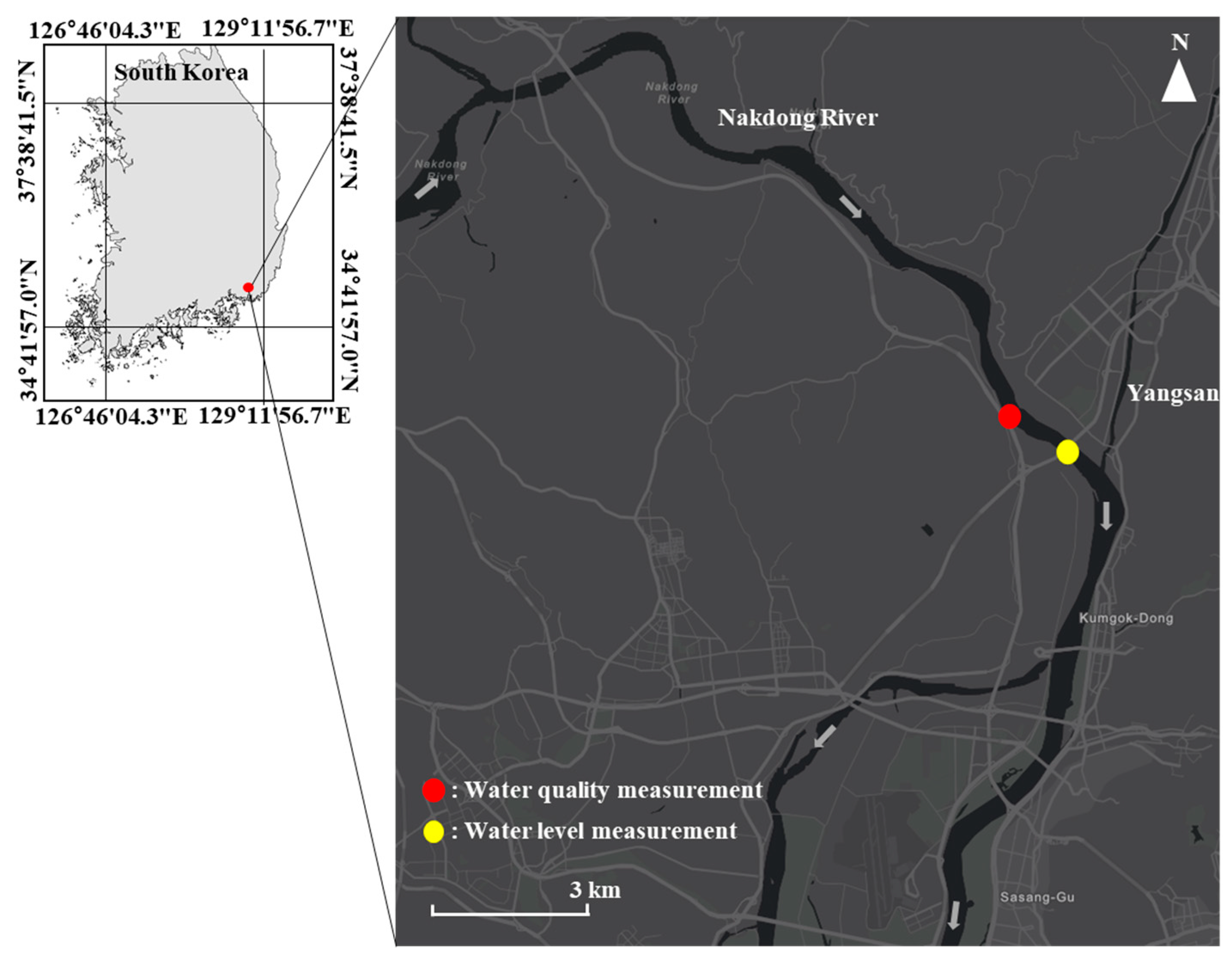
Water level data were collected from the Water Resources Management Information System (WAMIS) in South Korea, while water quality data were obtained from the Real-Time Water Quality Information (RTWQI) [14]. The water sampling and water level monitoring sites are displayed in Figure 1. The obtained water quality data included TP, TN and TOC. Additionally, the rainfall radar image and operation information of estuary barrage were acquired from the Korea Meteorological Administration (KMA) and the WAMIS, respectively. The entire simulation period was 1 January 2016–16 November 2017 and divided into two parts: (1) calibration period (1 January 2016–1 March 2017); and (2) validation period (2 March 2017–16 November 2017).
2.2. Water Level and Quality Simulation
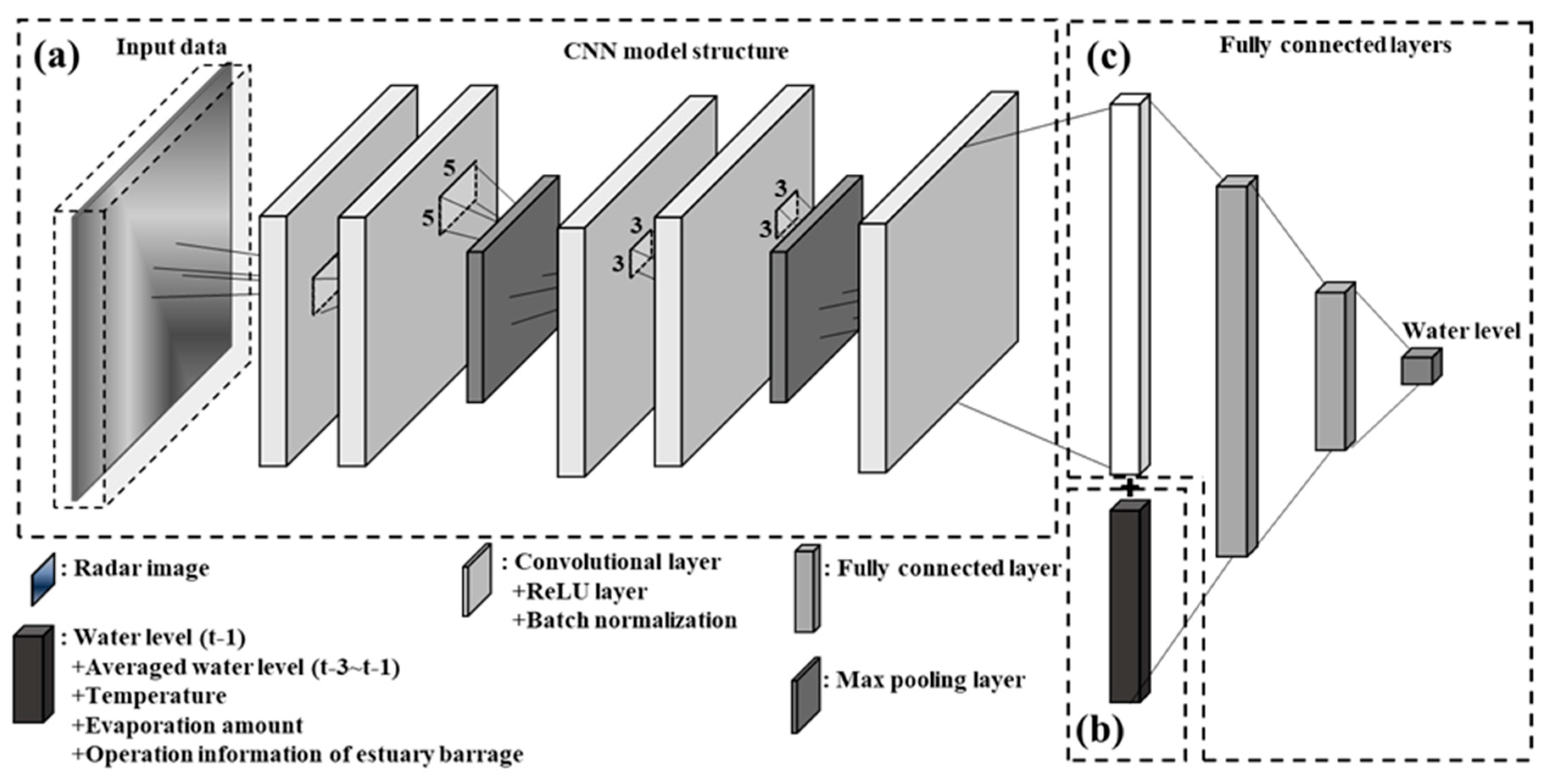
In this study, CNN and LSTM network were combined for predicting the water levels and water quality concentrations, respectively. CNN and LSTM are the most common algorithms among deep learning (DL) models and have applied to the various fields (e.g., image recognition, transition, and speech analysis) [15,16]. Specifically, CNN has been developed to recognize patterns of image features [17], while LSTM has been widely used for identifying patterns in sequential data such as time series [18]. Figure 2 shows our CNN model architecture with two inputs having different shapes: multi-dimensional and single vector data. The multi-dimensional data consisted of the rainfall radar image with the dimension 251 × 141 (Figure 2a), while the single vectors were applied as the additional information such as the water level in the previous day, the averaged water level for the past three days, the temperature, the operation information of estuary barrage and the evaporation (Figure 2b). Based on assumption that the water level of the Nakdong River Estuary Barrage can influence the water level at the water level monitoring site (Figure 1), because the Nakdong River Estuary Barrage is closed to the site, water levels of one control structure (the Nakdong River Estuary Barrage) were used for this study. The CNN model consisted of three convolutional layers, two max pooling and two fully connected layers. The output image from the convolutional layer and single vector data were fed into a fully connected layer that converts a one-dimensional feature vector (Figure 2c) [19]. The output from the fully connected layer was the water level. The more detailed descriptions for each layer in CNN are found in Section 2.3. A schematic diagram for LSTM is shown in Figure 3. The input data of this model adopted the water level and water quality concentrations in previous time step. This structure comprised LSTM and fully connected layers. The output from the LSTM layers transferred a fully connected layer, resulting in generating the concentrations of the water quality. More details on the LSTM layers are given in Section 2.4. Both CNN and LSTM models used the mean square error (MSE) as the loss function during the model training. The CNN and LSTM model were implemented using TensorFlow (1.4, Google brain, Mountain View, CA, USA) environment based on Python.
2.3. Convolutional Neural Network (CNN)
CNN recognizes the patterns to represent image features by utilizing the convolutional layers [17]. CNNs can receive images or a multi-dimensional matrix, and the neurons in CNN are connected to a smaller feature from the previous layer. This algorithm can reduce computations and prevent overfitting problems [20]. Therefore, CNN has been adopted in numerous studies focusing on the image objects from digital images [21]. A convolutional layer consists of the filter size, padding, and stride as the layer parameters [21]. The filter having a specific size (e.g., FH: filter height, FW: filter width) moves around the input image [22]. The padding inserts the zero values around the input image, which prevents the loss for the feature extraction [23]. The stride can define the step size of the filter in convolutions [24]. In each convolutional layer, the output size is calculated as:
where, OH is the height of output, IH is the height of input, FH is the height of the filter, SH is the height of the stride, OW is the width of output, IW is the width of input, PH is the height of the padding, PW is the width of the padding, FW is the width of the filter, and SW is the width direction of the stride [22].
In general, the convolutional layer needs the activation function to transform the signal from linear to non-linear. The rectified linear unit (ReLU) is employed as the activation function in this study. This function improves the computational speed and accuracy compared with the other activation functions (e.g., tangent sigmoid function) [25]. Especially, the ReLU function prevents the vanishing gradient problem by an exponentially decreasing the training gradient. The ReLU function is defined as:
where, is the output of ReLU and x is the input signal.
The max-pooling layer was used to extract the invariant features with an efficient convergence rate. This layer can eliminate the non-maximal values by the non-linear downsampling that can reduce the computational sampling during the CNN process [26]. The fully connected vector connects a loss function to calculate errors between the observed and simulated values by the vectorizing the input signal [27]. The MSE is used as a loss function in our study [28,29]. This calculates errors between simulated and observed values. The mathematical equation of the MSE is as follows:
where, is the simulated result, is the observed data, and N is the number of the dataset.
The stochastic gradient descent (SGD) optimization was applied to train a CNN network. SGD optimizes the parameters of a CNN network by reducing the loss function, as:
where, is the network parameter, is the training dataset, is the number of the dataset, and is the loss function.
The deep learning models such as CNN and LSTM require e an epoch number, a batch size, and a learning rate as the hyperparameters for the model training. The epoch number is the number of the learning in the entire training dataset, while the batch size is the number of samples that worked in the training at a time [30]. The learning rate is the step size at each iteration to minimize the loss function. In this study, the assigned epoch number and mini batch of CNN were 1000 and 16, respectively, and the applied learning rate was 0.001.
2.4. Long Short-Term Memory (LSTM)
The LSTM network is an extension of the recurrent neural network (RNN). RNN adopts a directed cycle structure that transfers the output of a hidden layer to the same hidden layer [31]. This structure can identify features of time-series by receiving the signal of the previous time. However, RNN has encountered the vanishing gradient problem, resulting in the unacceptable accuracy [18]. This vanishing gradient problem was overcome in LSTM suggested by Hochreiter and Schmidhuber [32]. The cell states can be updated by a gating regulation consisting of three different gates (forget gate, input gate, and output gate) and cells which are connected to each element. The following equations were used in LSTM:
where, is the cell state vector, is the activation function at time step t, is the input at current step t, is an element-wise non-linear activation function, is the input gate, is the forget gate, is the output gate, and is a cell state at current step t. The bias and weight matrices are represented as b and W, respectively.
2.5. Performance Evaluation
The accuracies of the predicted water level, TN, TP, and TOC were evaluated using coefficient of determination (R2), Nash–Sutcliffe efficiency (NSE) and mean square error (MSE). The equation of R2 and NSE is defined as follows:
where n is the number of datasets that have the water level (m), TN (mg/L), TP (mg/L) and TOC (mg/L), Pi indicates the predicted results, is mean of observed ones and Oi represents the observed data, is mean of observed ones.
3. Results and Discussion
3.1. Monitoring of Water Level and Water Quality
The results of the descriptive statistical analyses for the water level, TN, TP, and TOC are summarized in Table 1. In this study, the maximum values of water level, TN, TP and TOC were 1.19 m, 1.104, 0.003, and 2.100 mg/L, respectively, while the minimum values of those were 3.11 m, 4.383, 0.061, and 5.900 mg/L. The ratio of TN to TP (hereafter TN:TP ratio) was calculated using the minimum and Q2 values of TN and TP, respectively. The TN:TP ratio using those minimum values was 368 and that using the Q2 values was 150.62. The TN:TP ratio is an indicator of phytoplankton nutrient limitation [33]. These values were much higher than 22 of TN:TP ratio, indicating that NRB was in phosphorus-limited conditions [34,35]. The mean water level, TN, TP, and TOC were 1.65 m, 2.465, 0.021, and 3.202 mg/L, respectively. The median values of water level and TOC were close to the mean values of water level and TOC, while the median values of TN and TP were appreciably different from the mean values of those. The standard deviation of TN was the highest among the pollutants and TP had the highest coefficient of variation. Both statistics are commonly used to quantify the variation of data. However, the coefficient of variation is more proper to the comparison between the variations of each pollutant in that the coefficient of variation is useful to determine the variation of the independent data without considering the unit [36,37]. The water level of Q1 and Q3 were 1.60 and 1.69 (m), while the maximum water level was 3.11 (m), indicating that our data existed at the extreme value. This might be caused by the heavy rainfall that can provoke floods [38]. The validation set of water level and TOC smaller ranged than the training set of those, while these of TN and TP had a similar range to the training set. The standard deviation of the training set was larger than the validation set without TSS.
3.2. Water Level Simulation
Figure 4 presents a comparison between the observed and simulated water levels. The simulated water levels by the CNN model showed good agreement with the observed water levels. The R2 values between simulation and observation were 0.934 and 0.923 for the training and validation steps, respectively, while MSE between them were 0.001 and 0.001 (m2) (Table 2). The NSE values in the training and validation steps were 0.926 and 0.933, which is within the “very good” performance range (0.75 to 1) proposed by Moriasi et al. [39]. These values are in substantial agreement with those of Bustami et al. [40] and Panda et al. [41]. Bustami et al. [42] simulated water levels of the Bedup river in Malaysia using an artificial neural network (ANN) technique which resulted in an R2 value of 0.92. Panda et al. [41] produced the water levels of the Mahanadi delta using MIKE and ANN, by showing to R2 value of 0.921.
The water level fluctuated in the rainy season that is from June to October, while the variation of the water level was low in the dry season. This can be explained by considering that the rainfall was one of the most influential factors to the water level in that the increment of rainfall increased the water level [42]. Specifically, in the rainy season in 2016, the water level showed 3.11 m that was the highest value for the entire study period. The highest rainfall (407.7 mm) occurred in September of the year 2017. This heavy rainfall could result in a higher peak flow [38]. The CNN model in this study well captured this phenomenon, indicating that this model can simulate extreme water levels. The simulated results also showed relatively higher water levels in the rainy season in 2017 which were very similar to the observations. The water levels between the end of September and early October in 2016 were much higher than those for the same period in 2017. One possible explanation is that the period in the year 2016, typhoon Chava—one of the strongest tropical cyclones that made landfall in South Korea—had a great impact on the Korean peninsula with a large amount of precipitation.
3.3. Water Quality Simulation
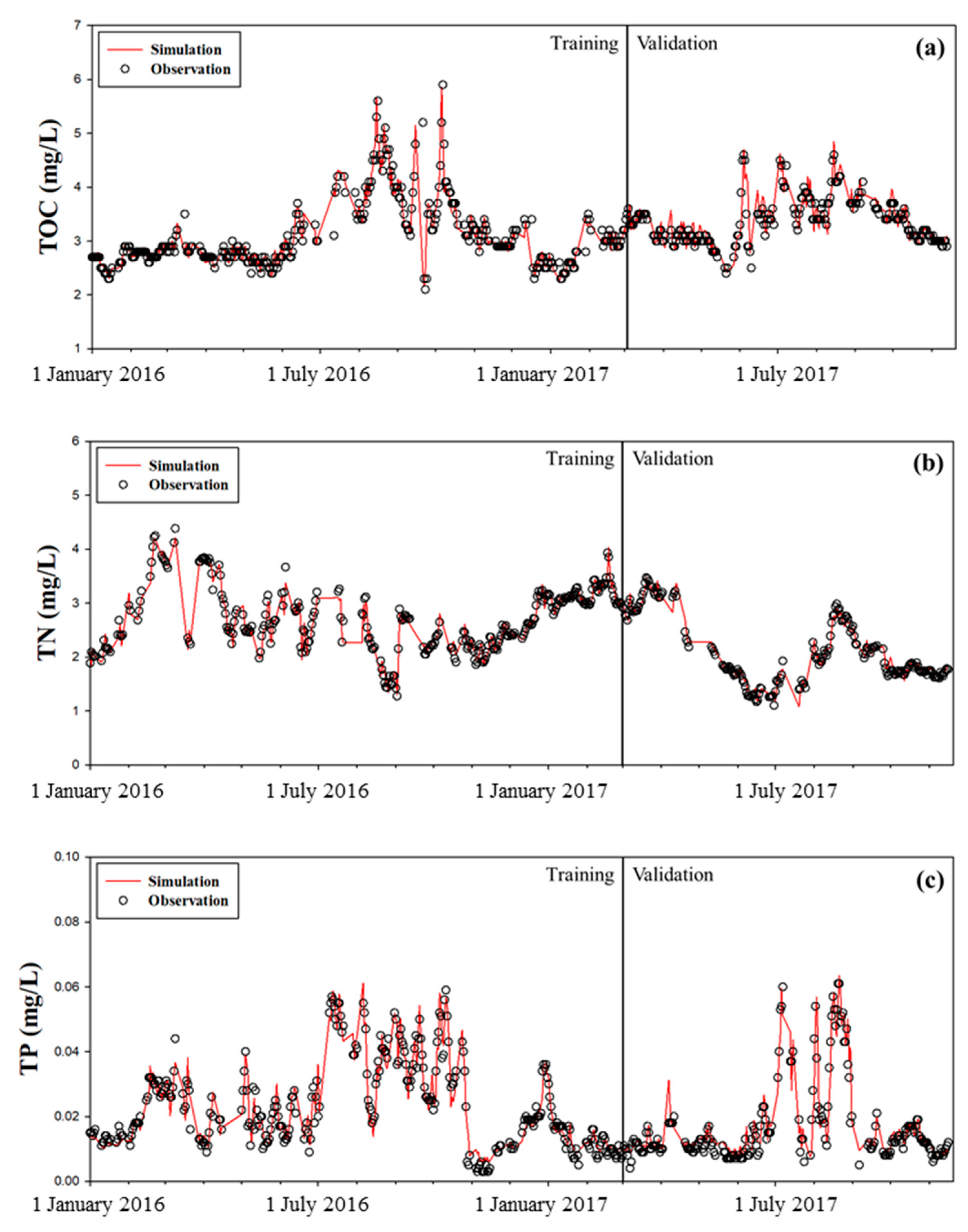
Figure 5 shows the comparison between the observed pollutant values and the simulated results of the LSTM model. The R2 of TP and TN for the training period were 0.92 and 0.95, respectively, while those in the validation period were 0.87 and 0.97, respectively (Table 2). TOC had the lowest R2 value among the pollutants for both of the training and validation periods, with 0.86 and 0.79, respectively. The MSE values for TOC, TN and TP for the training period were 1.37 × 10⁻⁵ 0.017 and 0.055 respectively, while those in the validation period were 2.08 × 10⁻⁵, 0.010 and 0.041, respectively. The NSE values of the LSTM model for both of the training and validation periods were above 0.75 which is within the “very good” performance range (0.75 to 1) in all the pollutants (e.g., TOC, TN and TP) [39]. As shown in Figure 5, the LSTM model in this study well simulated the temporal variations of those pollutants. Since these temporal variations may result from pollutant transport characteristics, this result implies that the LSTM model can properly reflect the transport characteristics of each pollutant. These temporal variations have been well simulated in previous studies. For example, Zhang et al. [43] predicted the temporal variations of DO in the Burnett river using the PCA-RNN model with the R2 value of 0.908. Choubin et al. [44] used the CART model to simulate the suspended solids in the Haraz River with an R2 value of 0.67. These studies focused on simulating a single pollutant, while our study simulated the concentrations of multiple pollutants (i.e., TOC, TN and TP).
The fluctuations of temporal variations in TOC and TP were higher in the rainy season (June to October) than those in the dry season. This can be explained by considering the rainfall patterns in South Korea. Most of the precipitation in South Korea falls in the summer monsoon season (June to September). TOC and TP were easily washed off by the rainfall resulting in higher concentrations of these pollutants in the rainy season [45,46]. Schrumrf et al. [47] demonstrated that TOC increased with rainfall. Park et al. [48] also showed that TP was higher in the rainy season compared with the dry season. However, the patterns of temporal variations for TN were different from the two pollutants. The TN concentrations increase in the period from February to June. We surmised that the nitrogen fertilizer application contributed to this increase. The fertilizers in South Korea are usually applied in spring and contain a large amount of nitrogen [49,50,51]. NRB has a broad agricultural area that can influence the variation of TN. Karlen et al. [52] reported that higher TN in water was generally found after fertilizer applications.
4. Conclusions and Future Work
In this study, we combined the two deep learning models (CNN and LSTM) to simulate the water level and the three water quality parameters (TN, TP and TOC) in NRB. Among the deep learning models, the CNN model was adopted to simulate the water level, while the LSTM model was selected to simulate the concentration of the pollutants. We found the following in this study:
- (1)
- The water level from the CNN model produced the NSE value of 0.933 that can be regarded as acceptable model performance. The water levels increased in the rainy season, while those were low in the dry season.
- (2)
- For all of the pollutants, the NSE values of the LSTM model for the training and validation periods were above 0.75 which is within the “very good” performance range. The LSTM model in this study well represented the different temporal variations of each pollutant type.
- (3)
- The TOC and TP concentrations had similar temporal variations in that the concentrations of the pollutants were highly fluctuated in the rainy season, while TN increased in the spring season.
This study suggests that the combined approach of the two deep learning techniques proposed in this study has promise as a tool in accurately simulating the water level and water quality and that this approach can contribute to developing effective strategies for better water sustainability and management. Although our model showed the acceptable model performance, only the three different pollutants were investigated in this study. However, most process-based models can simulate a lot more water quality including the three pollutants (e.g., chlorophyll, algae, dissolved oxygen, and fecal bacteria). A further study is recommended to develop deep learning models so that more pollutants including chlorophyll, algae, dissolved oxygen, and fecal bacteria can be simulated. In addition, further study on the deep learning model with “visual explanations” is required, such as Gradient-weighted-Class Activation Mapping (Grad-CAM) [53] and CAM [54], because the deep learning model is a black-box model that has general difficulty in identifying physical features. In addition, the approach outlined in this study should be replicated with other datasets.
Author Contributions
Conceptualization, S.-S.B. and J.A.C.; methodology, S.-S.B. and J.P.; formal analysis, S.-S.B. and J.P.; writing—original draft preparation, S.-S.B., J.P. and J.A.C.; writing—review and editing, S.-S.B., J.P. and J.A.C. All authors have read and agreed to the published version of the manuscript.
Funding
This study is supported by the APEC Climate Center.
Conflicts of Interest
The authors declare no conflict of interest.
References
- Arnold, J.G.; Moriasi, D.N.; Gassman, P.W.; Abbaspour, K.C.; White, M.J.; Srinivasan, R.; Santhi, C.; Harmel, R.D.; van Griensven, A.; Van Liew, M.W.; et al. SWAT: Model use, calibration, and validation. Trans. Asabe 2012, 55, 1491–1508. [Google Scholar] [CrossRef]
- Huber, W.C. Storm Water Management Model (SWMM) Bibliography; Environmental Research Laboratory, Office of Research and Development, U.S. Environmental Protection Agency: Cininnnati, OH, USA, 1985.
- Baek, S.; Ligaray, M.; Pyo, J.; Park, J.P.; Kang, J.H.; Pachepsky, Y.; Chun, J.A.; Cho, K.H. A novel water quality module of the SWMM model for assessing Low Impact Development (LID) in urban watersheds. J. Hydrol. 2020, 586, 124886. [Google Scholar] [CrossRef]
- Ahmed, A.N.; Othman, F.B.; Afan, H.A.; Ibrahim, R.K.; Fai, C.M.; Hossain, M.S.; Ehteram, M. Machine learning methods for better water quality prediction. J. Hydrol. 2019, 578, 124084. [Google Scholar] [CrossRef]
- Almalaq, A.; Zhang, J.J. Deep learning application: Load forecasting in big data of smart grids. In Deep Learning: Algorithms and Applications; Pedryca, W., Chen, S.M., Eds.; Springer: Cham, Switzerland, 2020; pp. 103–128. [Google Scholar]
- Liu, P.; Wang, J.; Sangaiah, A.K.; Xie, Y.; Yin, X. Analysis and prediction of water quality using LSTM deep neural networks in IoT environment. Sustainability 2019, 11, 2058. [Google Scholar] [CrossRef] [Green Version]
- Hu, Z.; Zhang, Y.; Zhao, Y.; Xie, M.; Zhong, J.; Tu, Z.; Liu, J. A water quality prediction method based on the deep LSTM network considering correlation in smart mariculture. Sensors 2019, 19, 1420. [Google Scholar] [CrossRef] [PubMed] [Green Version]
- Barzegar, R.; Aalami, M.T.; Adamowsk, J. Short-term water quality variable prediction using a hybrid CNN-LSTM deep learning model. Stoch. Environ. Res. Risk. Assess. 2020, 34, 415–433. [Google Scholar] [CrossRef]
- K-Water. Dam Operation Practice Manual; K-Water: Daejeon, Korea, 2013. (In Korean) [Google Scholar]
- Nakdong River Environmental Management Office. Water Quality Conservation Strategies for the Greater Nakdong River Region, ’93–97 Implementation Status and Evaluation; Nakdong River Environmental Management Office: Changwon, Korea, 1998. [Google Scholar]
- Seo, M.; Lee, H.; Kim, Y. Relationship between Coliform Bacteria and Water Quality Factors at Weir Stations in the Nakdong River, South Korea. Water 2019, 11, 1171. [Google Scholar] [CrossRef] [Green Version]
- Kim, S.; Park, S.; Kim, H. Waste Load Allocation Study for a Large River System; Korea Environment Institute: Seoul, Korea, 1998. (In Korean) [Google Scholar]
- Park, S.S.; Lee, Y.S. A water quality modeling study of the Nakdong River, Korea. Ecol. Model. G 2002, 152, 65–75. [Google Scholar] [CrossRef]
- WAMIS. Available online: http://www.wamis.go/kr/ (accessed on 9 October 2020).
- Xudong, H.; Xiao, Z.; Jinyuan, X.; Linna, W.; Wei, X. Cross-Lingual Non-Ferrous Metals Related News Recognition Method Based on CNN with A Limited Bi-Lingual Dictionary. Comput. Mater. Contin. 2019, 58, 379–389. [Google Scholar]
- Jin, W.; Yongsong, Z.; Lei, P.; Lei, W.; Osama, A.; Amr, T. Research on Crack Opening Prediction of Concrete Dam based on Recurrent Neural Network. J. Internet Technol. 2020, 21, 1161–1170. [Google Scholar]
- Deng, J.; Dong, W.; Socher, R.; Li, L.J.; Li, K.; Fei-Fei, L. Imagenet: A large-scale hierarchical image database. In Proceedings of the 2009 IEEE Conference on Computer Vision and Pattern Recognition, Miami, FL, USA, 20–25 June 2009; pp. 248–255. [Google Scholar]
- Yatian, S.; Yan, L.; Jun, S.; Wenke, D.; Xianjin, S.; Lei, Z.; Xiajiong, S.; Jing, H. Hashtag Recommendation Using LSTM Networks with Self-Attention. Comput. Mater. Continua 2019, 61, 1261–1269. [Google Scholar]
- Ioffe, S.; Szegedy, C. Batch normalization: Accelerating deep network training by reducing internal covariate shift. arXiv 2015, arXiv:1502.03167. [Google Scholar]
- Goodfellow, I.; Bengio, Y.; Courville, A.; Bengio, Y. Deep Learning; MIT Press: Cambridge, UK, 2016; Volume 1. [Google Scholar]
- Ciresan, D.C.; Meier, U.; Masci, J.; Gambardella, L.M.; Schmidhuber, J. Flexible, high performance convolutional neural networks for image classification. In Proceedings of the Twenty-Second International Joint Conference on Artificial Intelligence, Manno-Lugano, Switzerland, 16–22 July 2011; pp. 1237–1242. [Google Scholar]
- Krizhevsky, A.; Sutskever, I.; Hinton, G.E. Imagenet classification with deep convolutional neural networks. In Proceedings of the Advances in Neural Information Processing Systems, Lake Tahoe, NV, USA, 3–6 December 2012; pp. 1097–1105. [Google Scholar]
- Dumoulin, V.; Visin, F. A guide to convolution arithmetic for deep learning. arXiv 2016, arXiv:1603.07285. [Google Scholar]
- Acharya, U.R.; Fujita, H.; Lih, O.S.; Hagiwara, Y.; Tan, J.H.; Adam, M. Automated detection of arrhythmias using different intervals of tachycardia ECG segments with convolutional neural network. Inf. Sci. 2017, 405, 81–90. [Google Scholar] [CrossRef]
- Nair, V.; Hinton, G.E. Rectified linear units improve restricted boltzmann machines. In Proceedings of the 27th International Conference on Machine Learning (ICML-10), Haifa, Israel, 21–24 June 2010; pp. 807–814. [Google Scholar]
- Nagi, J.; Ducatelle, F.; Di Caro, G.A.; Cireşan, D.; Meier, U.; Giusti, A.; Nagi, F.; Schmidhuber, J.; Gambardella, L.M. Max-pooling convolutional neural networks for vision-based hand gesture recognition. In Proceedings of the 2011 IEEE International Conference on Signal and Image Processing Applications (ICSIPA), Manno-Lugano, Switzerland, 16–18 November 2011; pp. 342–347. [Google Scholar]
- Wu, J.N. Compression of fully-connected layer in neural network by kronecker product. In Proceedings of the 2016 Eighth International Conference on Advanced Computational Intelligence (ICACI), Chiang Mai, Thailand, 14–16 February 2016; pp. 173–179. [Google Scholar]
- Srivastava, H.M.; Gaboury, S.; Ghanim, F. A unified class of analytic functions involving a generalization of the Srivastava–Attiya operator. Appl. Math. Comput. 2015, 251, 35–45. [Google Scholar] [CrossRef]
- Heinermann, J.; Kramer, O. Machine learning ensembles for wind power prediction. Renew. Energy 2016, 89, 671–679. [Google Scholar] [CrossRef]
- Robert, C. Machine Learning, a Probabilistic Perspective; Taylor & Francis: Abingdon, UK, 2014. [Google Scholar]
- Salehinejad, H.; Sankar, S.; Barfett, J.; Colak, E.; Valaee, S. Recent advances in recurrent neural networks. arXiv 2017, arXiv:1801.01078. [Google Scholar]
- Hochreiter, S.; Schmidhuber, J. Long short-term memory. Neural Comput. 1997, 9, 1735–1780. [Google Scholar] [CrossRef]
- Wang, H.J.; Liang, X.M.; Jiang, P.H.; Wang, J.; Wu, S.K.; Wang, H.Z. TN: TP ratio and planktivorous fish do not affect nutrient-chlorophyll relationships in shallow lakes. Freshw. Biol. 2008, 53, 935–944. [Google Scholar] [CrossRef]
- Guildford, S.J.; Hecky, R.E. Total nitrogen, total phosphorus, and nutrient limitation in lakes and oceans: Is there a common relationship? Limnol. Oceanogr. 2000, 45, 1213–1223. [Google Scholar] [CrossRef] [Green Version]
- Park, Y.; Cho, K.H.; Park, J.; Cha, S.M.; Kim, J.H. Development of early-warning protocol for predicting chlorophyll-a concentration using machine learning models in freshwater and estuarine reservoirs, Korea. Sci. Total Environ. 2015, 502, 31–41. [Google Scholar] [CrossRef] [PubMed]
- Reed, G.F.; Lynn, F.; Meade, B.D. Use of coefficient of variation in assessing variability of quantitative assays. Clin. Diagn. Lab. Immunol. 2002, 9, 1235–1239. [Google Scholar] [CrossRef] [PubMed] [Green Version]
- Abdi, H. Coefficient of variation. Encycl. Res. Des. 2010, 1, 169–171. [Google Scholar]
- Krvavica, N.; Rubinić, J. Evaluation of Design Storms and Critical Rainfall Durations for Flood Prediction in Partially Urbanized Catchments. Water 2020, 12, 2044. [Google Scholar] [CrossRef]
- Moriasi, D.N.; Arnold, J.G.; Van Liew, M.W.; Bingner, R.L.; Harmel, R.D.; Veith, T.L. Model evaluation guidelines for systematic quantification of accuracy in watershed simulations. Trans. Asabe 2007, 50, 885–900. [Google Scholar] [CrossRef]
- Bustami, R.; Bessaih, N.; Bong, C.; Suhaili, S. Artificial Neural Network for Precipitation and Water Level Predictions of Bedup River. Iaeng Int. J. Comput. Sci. 2007, 34, 228–233. [Google Scholar]
- Panda, R.K.; Pramanik, N.; Bala, B. Simulation of river stage using artificial neural network and MIKE 11 hydrodynamic model. Comput. Geosci. 2010, 36, 735–745. [Google Scholar] [CrossRef]
- Lee, L.; Lawrence, D.; Price, M. Analysis of water-level response to rainfall and implications for recharge pathways in the Chalk aquifer, SE England. J. Hydrol. 2006, 330, 604–620. [Google Scholar] [CrossRef]
- Zhang, Y.F.; Fitch, P.; Thorburn, P.J. Predicting the Trend of Dissolved Oxygen Based on the kPCA-RNN Model. Water 2020, 12, 585. [Google Scholar] [CrossRef] [Green Version]
- Choubin, B.; Darabi, H.; Rahmati, O.; Sajedi-Hosseini, F.; Kløve, B. River suspended sediment modelling using the CART model: A comparative study of machine learning techniques. Sci. Total Environ. 2018, 615, 272–281. [Google Scholar] [CrossRef]
- Parks, S.J.; Baker, L.A. Sources and transport of organic carbon in an Arizona river-reservoir system. Water Res. 1997, 31, 1751–1759. [Google Scholar] [CrossRef]
- Alamdari, N.; Sample, D.J.; Steinberg, P.; Ross, A.C.; Easton, Z.M. Assessing the effects of climate change on water quantity and quality in an urban watershed using a calibrated stormwater model. Water 2017, 9, 464. [Google Scholar] [CrossRef]
- Schrumpf, M.; Zech, W.; Lehmann, J.; Lyaruu, H.V. TOC, TON, TOS and TOP in rainfall, throughfall, litter percolate and soil solution of a montane rainforest succession at Mt. Kilimanjaro, Tanzania. Biogeochemistry 2006, 78, 361–387. [Google Scholar] [CrossRef]
- Park, M.; Choi, Y.S.; Shin, H.J.; Song, I.; Yoon, C.G.; Choi, J.D.; Yu, S.J. A comparison study of runoff characteristics of non-point source pollution from three watersheds in South Korea. Water 2019, 11, 966. [Google Scholar] [CrossRef] [Green Version]
- Cao, P.; Lu, C.C.; Yu, Z. Historical nitrogen fertilizer use in agricultural ecosystems of the contiguous United States during 1850–2015: Application rate, timing, and fertilizer types. Earth Syst. Sci. Data 2018, 10, 969–984. [Google Scholar] [CrossRef] [Green Version]
- Kim, J.G.; Chung, E.S.; Seo, S.; Kim, M.J.; Chang, Y.S.; Chung, B.C. Effect of nitrogen fertilizer level and mixture of small grain and forage rape on productivity and quality of spring at South Region in Korea. J. Korean Soc. Grasl. Forage Sci. 2005, 25, 143–150. (In Korean) [Google Scholar]
- RDA. Available online: http://www.rda.go.kr/foreign/ten/ (accessed on 9 October 2020).
- Karlen, D.L.; Dinnes, D.L.; Jaynes, D.B.; Hurburgh, C.R.; Cambardella, C.A.; Colvin, T.S.; Rippke, G.R. Corn response to late-spring nitrogen management in the Walnut Creek watershed. Agron. J. 2005, 97, 1054–1061. [Google Scholar] [CrossRef] [Green Version]
- Selvaraju, R.R.; Cogswell, M.; Das, A.; Vedantam, R.; Parikh, D.; Batra, D. Grad-cam: Visual explanations from deep networks via gradient-based localization. In Proceedings of the IEEE International Conference on Computer Vision, Venice, Italy, 22–29 October 2017; pp. 618–626. [Google Scholar]
- Zhou, B.; Khosla, A.; Lapedriza, A.; Oliva, A.; Torralba, A. Learning deep features for discriminative localization. In Proceedings of the IEEE Conference on Computer Vision and Pattern Recognition, Las Vegas, NV, USA, 27–30 June 2016; pp. 2921–2929. [Google Scholar]
Figure 1.
Study area and water sampling and water level monitoring sites in the Nakdong River Basin (NRB) in South Korea.
Figure 1.
Study area and water sampling and water level monitoring sites in the Nakdong River Basin (NRB) in South Korea.

Figure 2.
Convolutional neural network (CNN) architectures for simulating the water level: (a) convolutional layer for radar images, (b) additional information (e.g., water level in the previous day, the averaged water level for the past three days, temperature, operation information of estuary barrage and evaporation), and (c) fully connected layer.

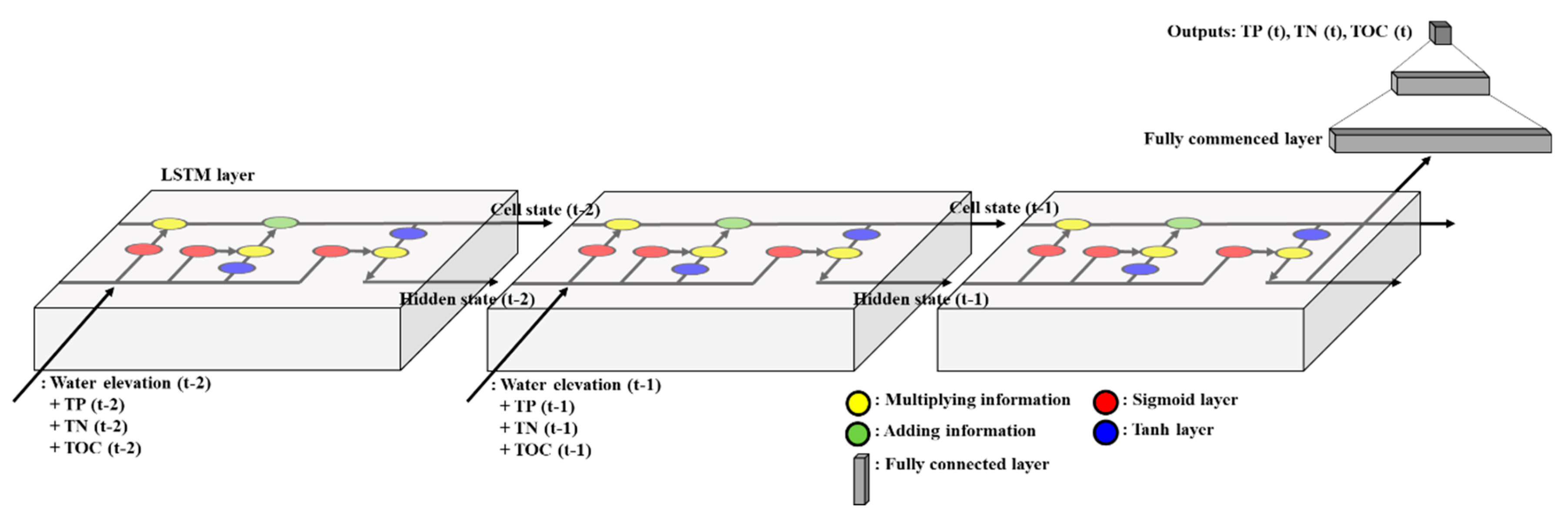
Figure 3.
Architecture of the proposed Long Short-Term Memory (LSTM) model in this study, consisting of an LSTM and a fully connected layer to simulate the water quality concentrations.
Figure 3.
Architecture of the proposed Long Short-Term Memory (LSTM) model in this study, consisting of an LSTM and a fully connected layer to simulate the water quality concentrations.

Figure 4.
Comparison of the observed and simulated water level for the study period: (a) training and (b) validation periods.
Figure 4.
Comparison of the observed and simulated water level for the study period: (a) training and (b) validation periods.
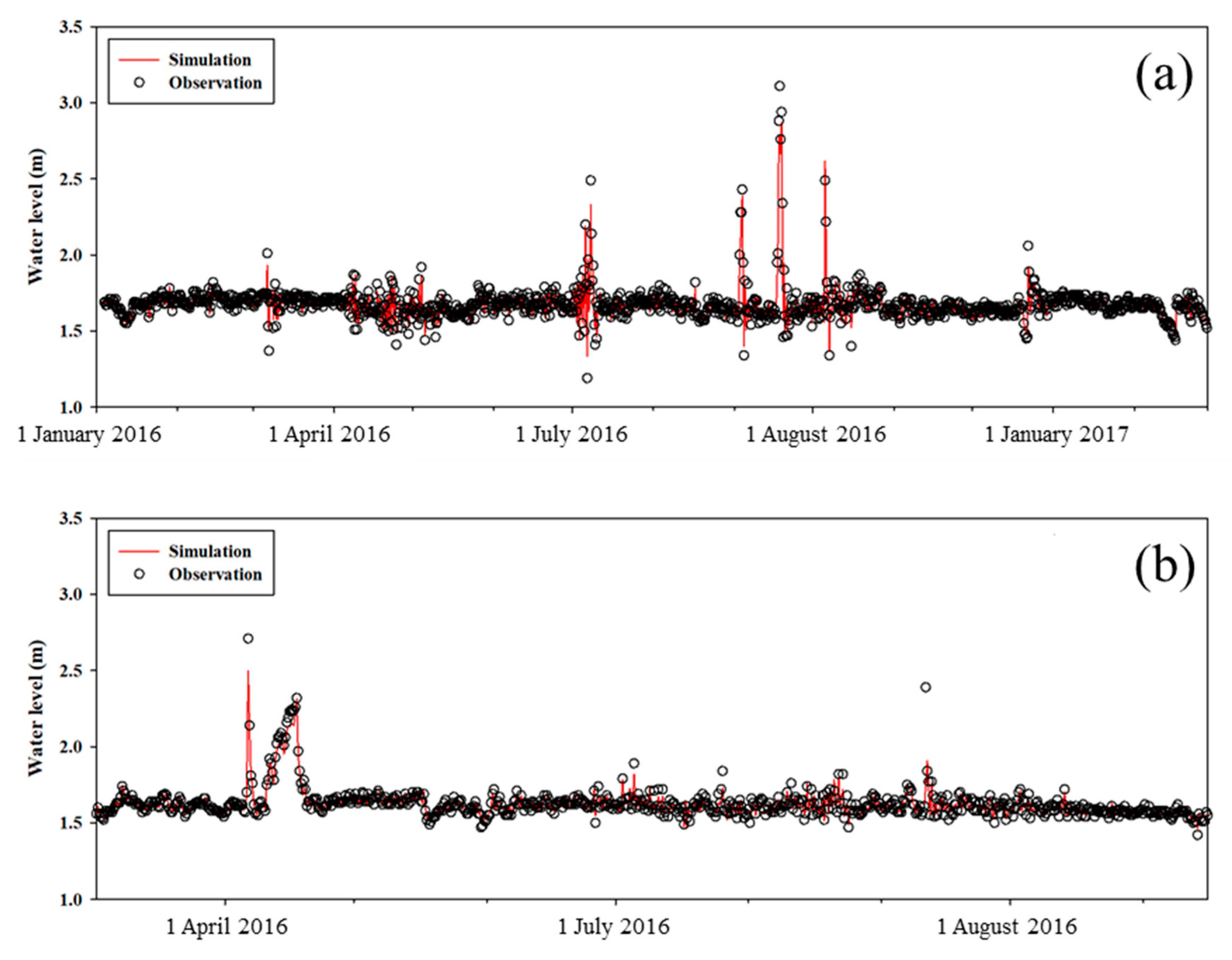
Figure 5.
Comparison of the observed and simulated pollutants: (a) TOC, (b) TN and (c) TP.

Table 1.
Descriptive statistics of water level, total nitrogen (TN), total organic carbon (TOC), and total phosphorus (TP).
Table 1.
Descriptive statistics of water level, total nitrogen (TN), total organic carbon (TOC), and total phosphorus (TP).
| Periods | Descriptive Statistics | Water Level (m) | TN (mg/L) | TP (mg/L) | TOC (mg/L) | |
|---|---|---|---|---|---|---|
| Total | Min | 1.19 | 1.104 | 0.003 | 2.100 | |
| Max | 3.11 | 4.383 | 0.061 | 5.900 | ||
| Mean | 1.65 | 2.465 | 0.021 | 3.202 | ||
| Median | 1.64 | 1.917 | 0.011 | 3.100 | ||
| Quantile | Q2 (25%) | 1.60 | 2.410 | 0.016 | 2.800 | |
| Q3 (75%) | 1.69 | 3.002 | 0.028 | 3.500 | ||
| Standard deviation | 0.12 | 0.666 | 0.013 | 0.577 | ||
| CoV | 0.07 | 0.270 | 0.646 | 0.180 | ||
| Training | Min | 1.19 | 1.274 | 0.003 | 2.100 | |
| Max | 3.11 | 4.383 | 0.059 | 5.900 | ||
| Mean | 1.68 | 2.706 | 0.023 | 3.100 | ||
| Median | 1.67 | 2.660 | 0.020 | 2.900 | ||
| Quantile | Q2 (25%) | 1.63 | 2.252 | 0.013 | 2.700 | |
| Q3 (75%) | 1.71 | 3.096 | 0.031 | 3.300 | ||
| Standard deviation | 0.11 | 0.589 | 0.013 | 0.636 | ||
| CoV | 0.07 | 0.218 | 0.564 | 0.205 | ||
| Validation | Min | 1.36 | 1.104 | 0.004 | 2.400 | |
| Max | 2.71 | 3.473 | 0.061 | 4.600 | ||
| Mean | 1.62 | 2.105 | 0.017 | 3.366 | ||
| Median | 1.61 | 1.866 | 0.012 | 3.300 | ||
| Quantile | Q2 (25%) | 1.57 | 1.681 | 0.009 | 3.100 | |
| Q3 (75%) | 1.64 | 2.671 | 0.017 | 3.600 | ||
| Standard deviation | 0.11 | 0.610 | 0.013 | 0.417 | ||
| CoV | 0.07 | 0.290 | 0.762 | 0.124 | ||
Table 2.
Performance index of water level and water quality simulation.
| Periods | Index | Water Level (m) | TN (mg/L) | TP (mg/L) | TOC (mg/L) |
|---|---|---|---|---|---|
| Training | R2 | 0.934 | 0.950 | 0.92 | 0.860 |
| MSE | 0.001 | 0.017 | 1.37 × 10⁻⁵ | 0.055 | |
| NSE | 0.926 | 0.951 | 0.921 | 0.864 | |
| Validation | R2 | 0.923 | 0.970 | 0.87 | 0.793 |
| MSE | 0.001 | 0.010 | 2.08 × 10⁻⁵ | 0.041 | |
| NSE | 0.933 | 0.987 | 0.899 | 0.832 |
Publisher’s Note: MDPI stays neutral with regard to jurisdictional claims in published maps and institutional affiliations. |
© 2020 by the authors. Licensee MDPI, Basel, Switzerland. This article is an open access article distributed under the terms and conditions of the Creative Commons Attribution (CC BY) license (http://creativecommons.org/licenses/by/4.0/).
Share and Cite
MDPI and ACS Style
Baek, S.-S.; Pyo, J.; Chun, J.A. Prediction of Water Level and Water Quality Using a CNN-LSTM Combined Deep Learning Approach. Water 2020, 12, 3399. https://doi.org/10.3390/w12123399
AMA Style
Baek S-S, Pyo J, Chun JA. Prediction of Water Level and Water Quality Using a CNN-LSTM Combined Deep Learning Approach. Water. 2020; 12(12):3399. https://doi.org/10.3390/w12123399
Chicago/Turabian StyleBaek, Sang-Soo, Jongcheol Pyo, and Jong Ahn Chun. 2020. "Prediction of Water Level and Water Quality Using a CNN-LSTM Combined Deep Learning Approach" Water 12, no. 12: 3399. https://doi.org/10.3390/w12123399
Note that from the first issue of 2016, this journal uses article numbers instead of page numbers. See further details here.