Possibility of Zhuhai-1 Hyperspectral Imagery for Monitoring Salinized Soil Moisture Content Using Fractional Order Differentially Optimized Spectral Indices


Abstract
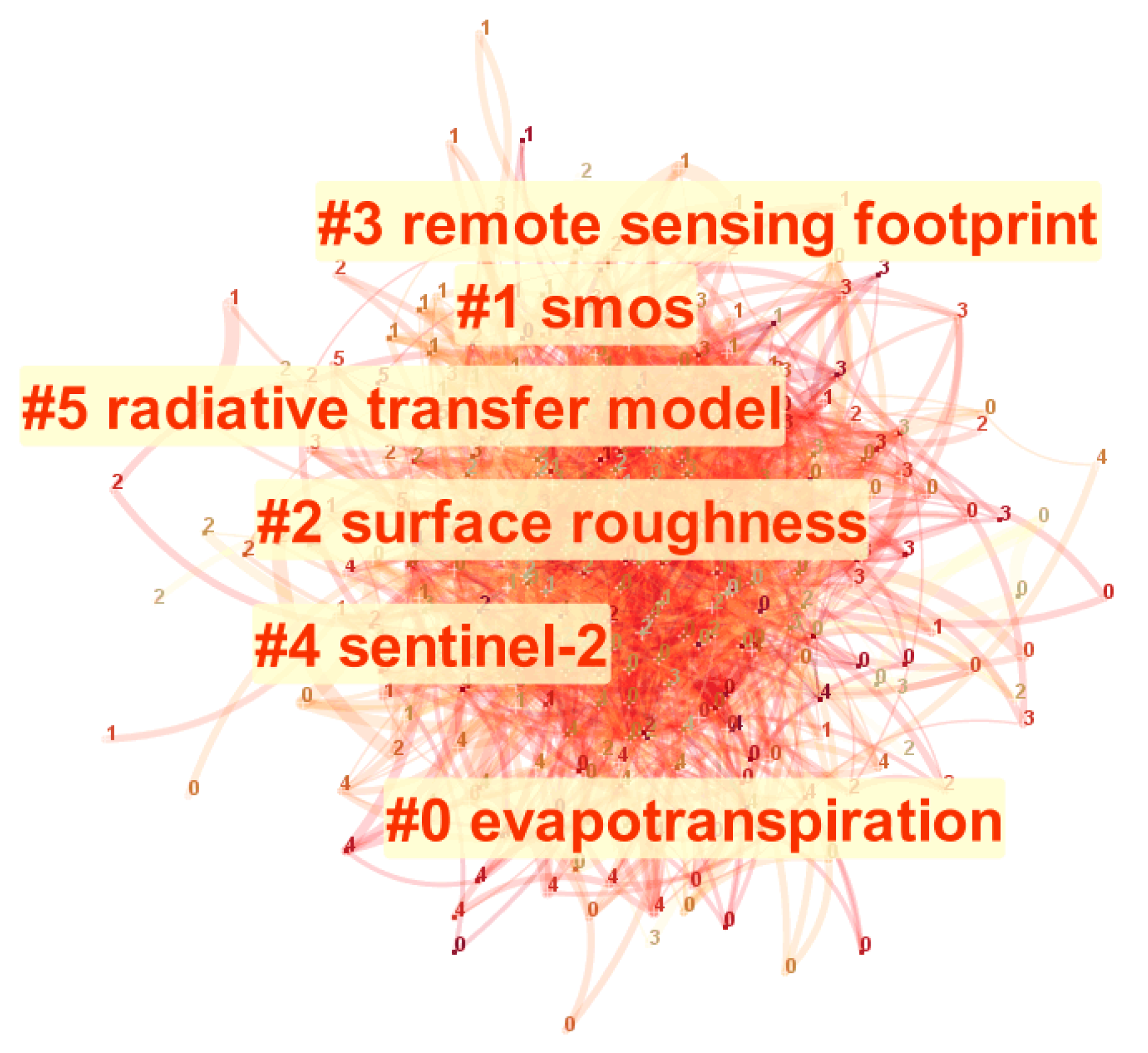
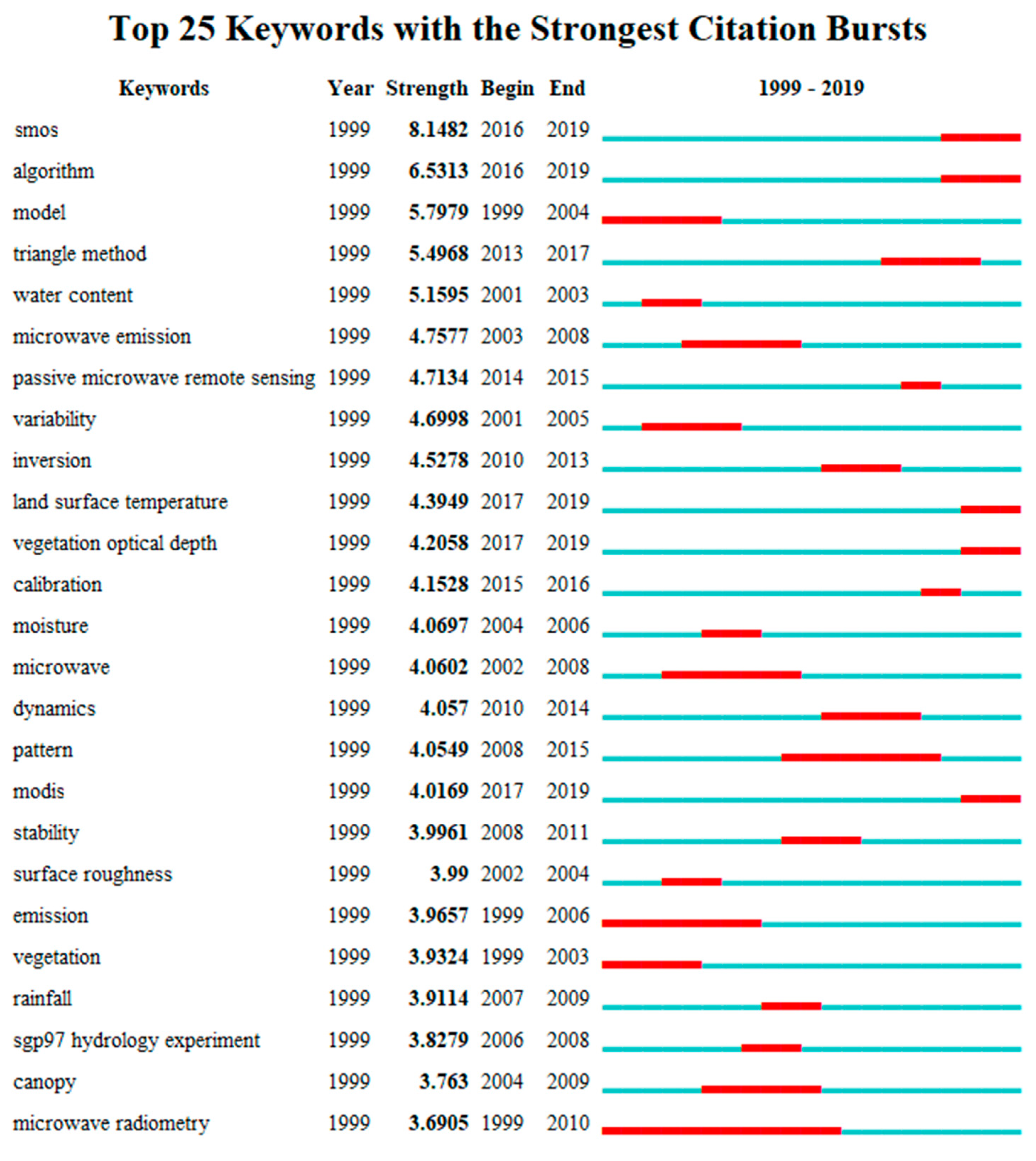
:1. Introduction
2. Materials and Methods
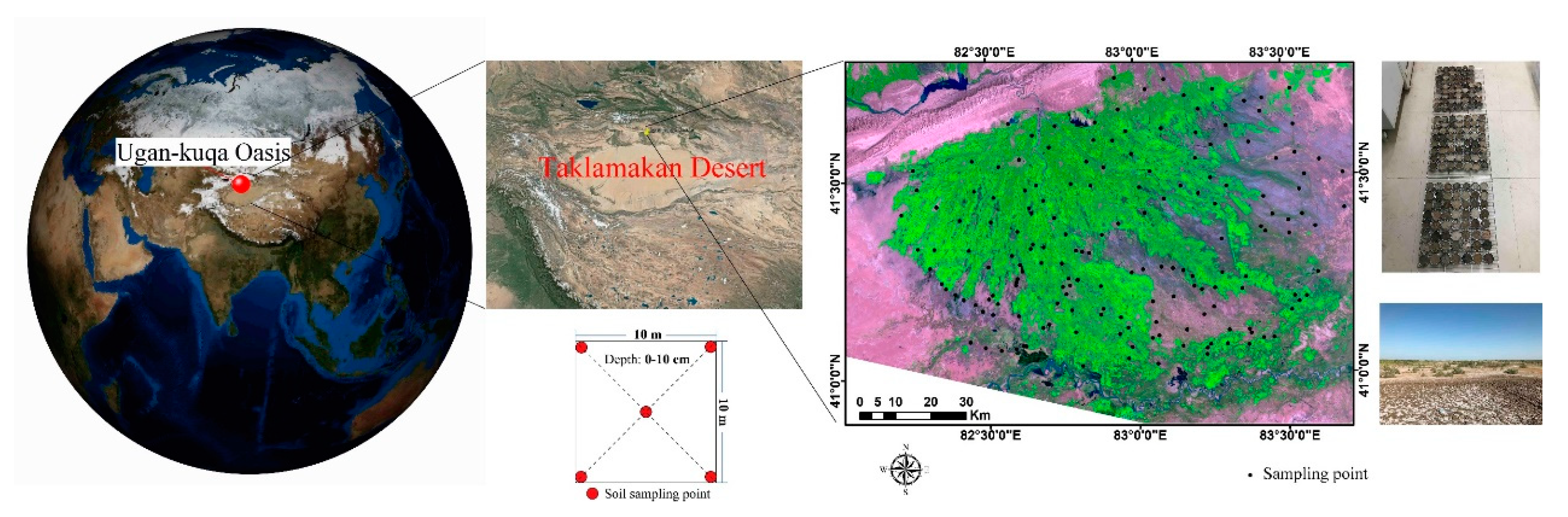
2.1. Study Area and Sampling Sites
2.2. Data Collection
2.2.1. Field Sampling and Spectral Measurements
2.2.2. Zhuhai-1 Hyperspectral Imagery
2.3. Fractional Order Differential Method
2.4. Optimized Spectral Indices Method
2.4.1. Two-Band Spectral Indices
2.4.2. Three-Band Spectral Indices
2.5. Modelling Strategies
2.5.1. Optimal Variable Selection Method
- (1)
- PCC method
- (2)
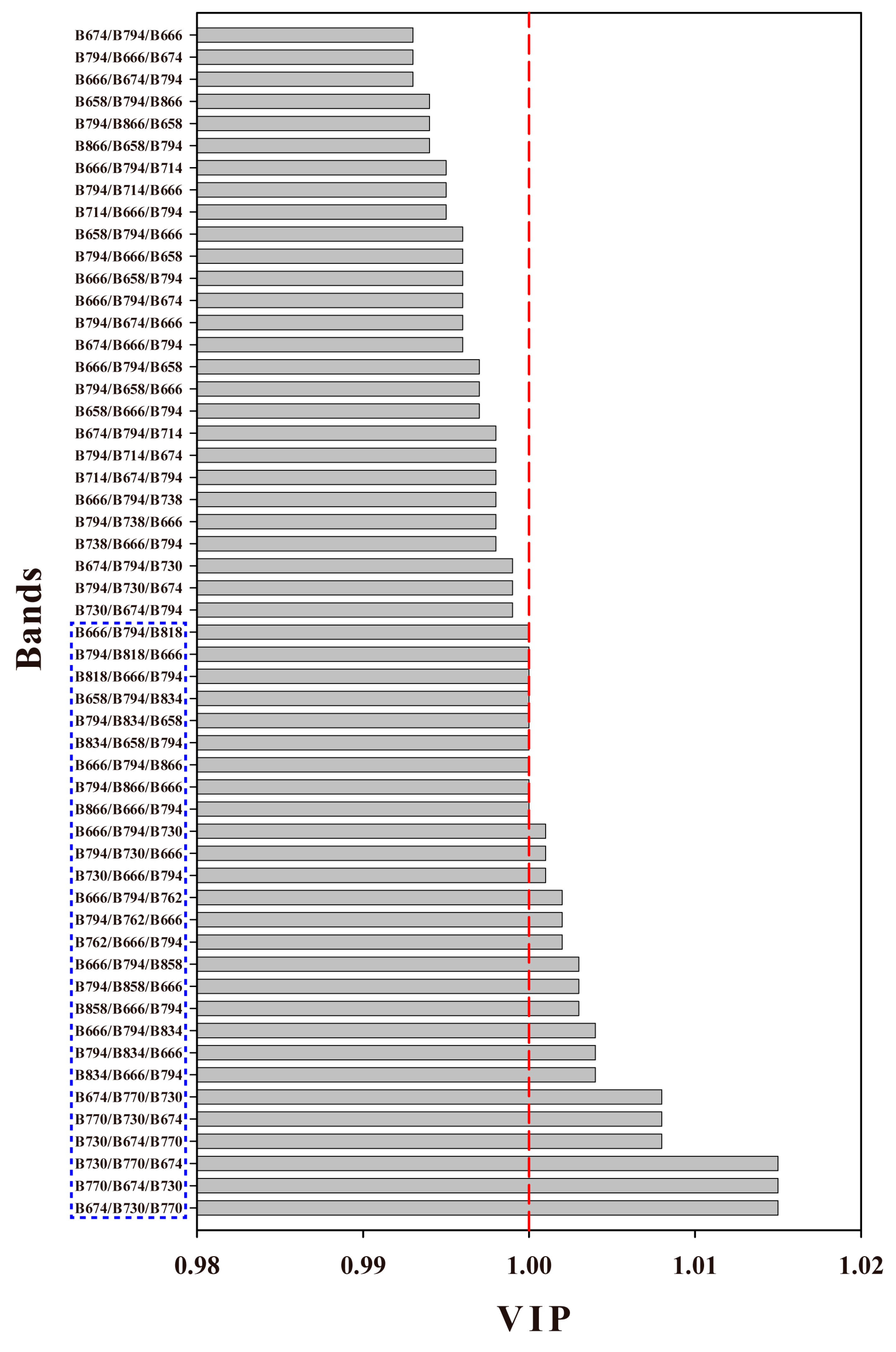
- VIP method
2.5.2. Modeling Approaches
- (1)
- MLR model
- (2)
- PR model
- (3)
- NR model
- (4)
- PLSR model
- (5)
- CART model
- (6)
- RF regression model
- (7)
- MARS model
- (8)
- TGBM regression model
2.5.3. Comparison of Model Accuracy
3. Results
3.1. Analysis of SMC and Hyperspectral Characteristics
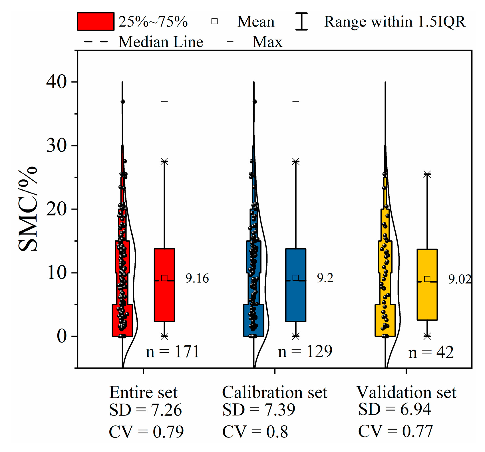
3.1.1. Descriptive Statistical Analysis of SMC
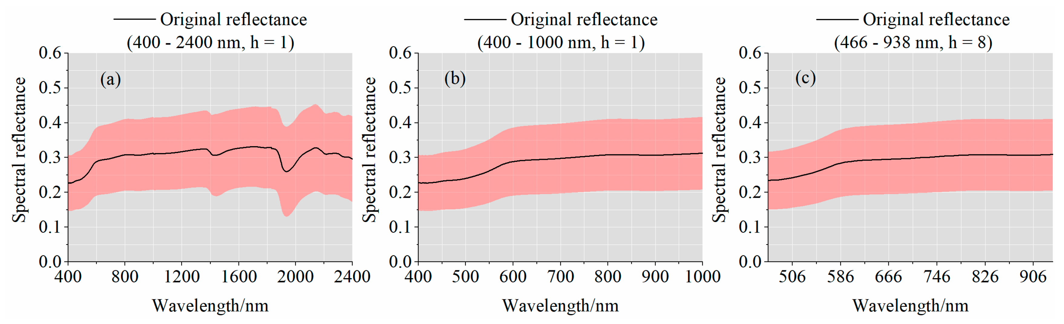
3.1.2. Soil Hyperspectral Characteristics Analysis
- (1)
- Soil average spectral curve analysis
- (2)
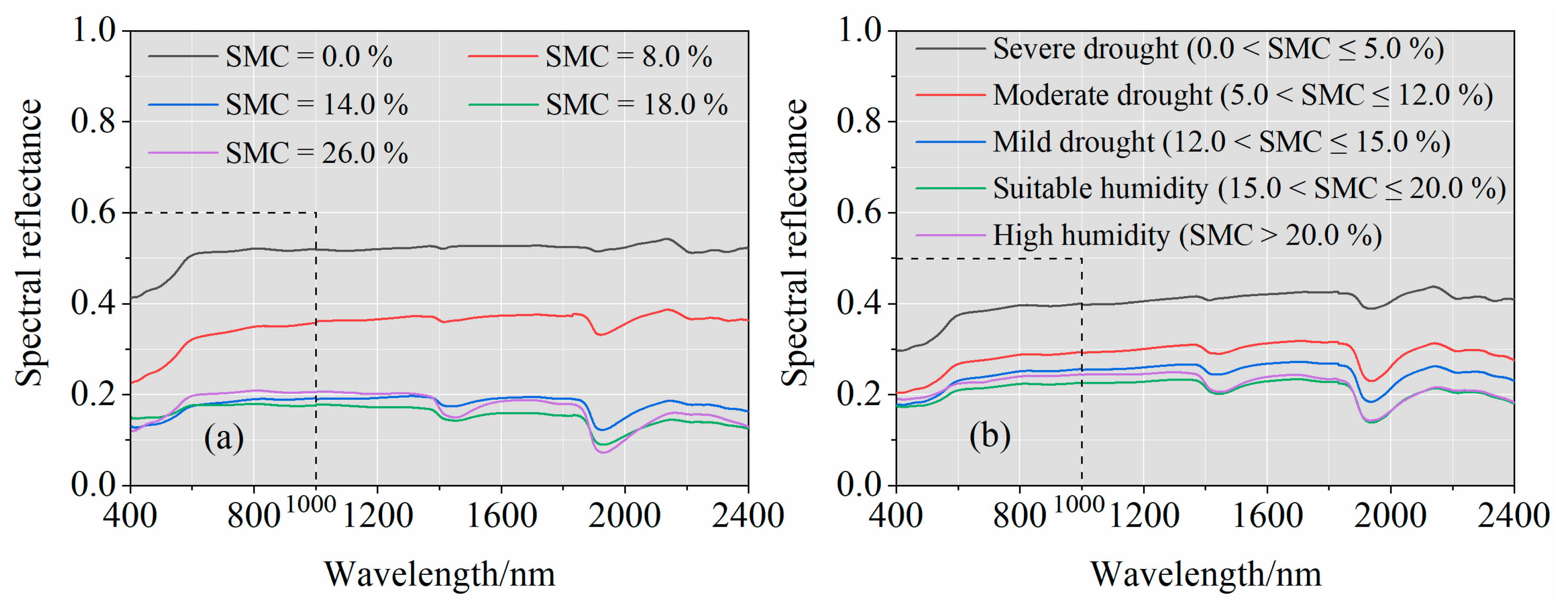
- Analysis of soil spectral characteristics under different humidity conditions
- (3)
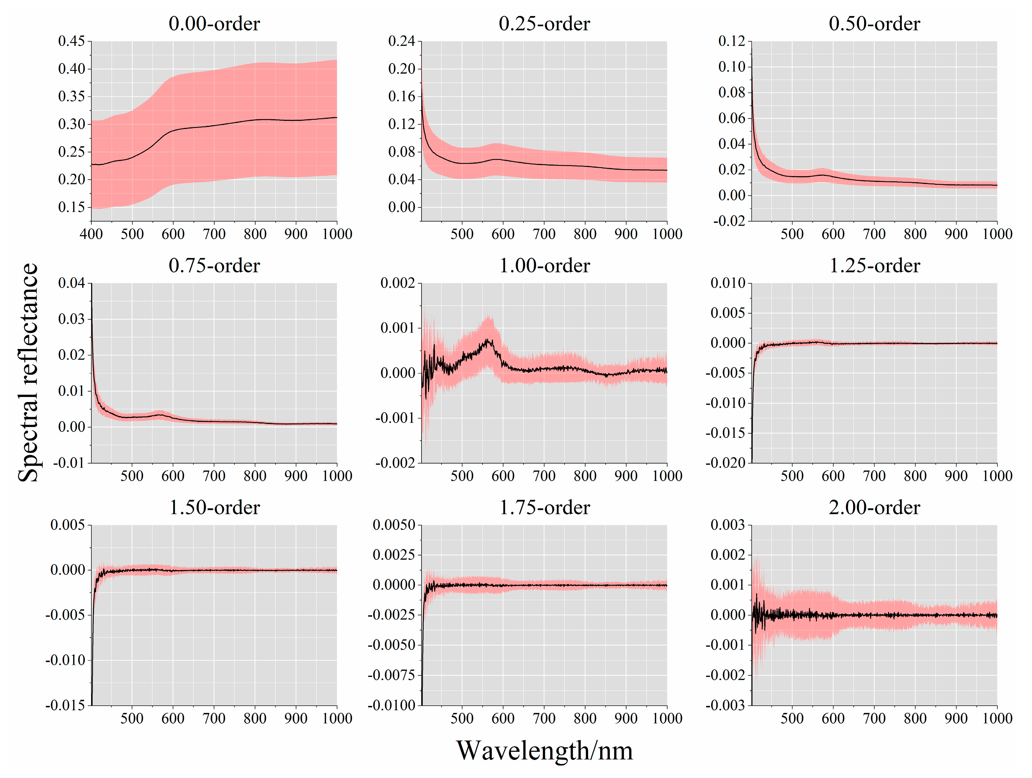
- Analysis of soil spectral characteristics of different fractional differential orders
3.2. PCC Analysis of SMC and Spectrum
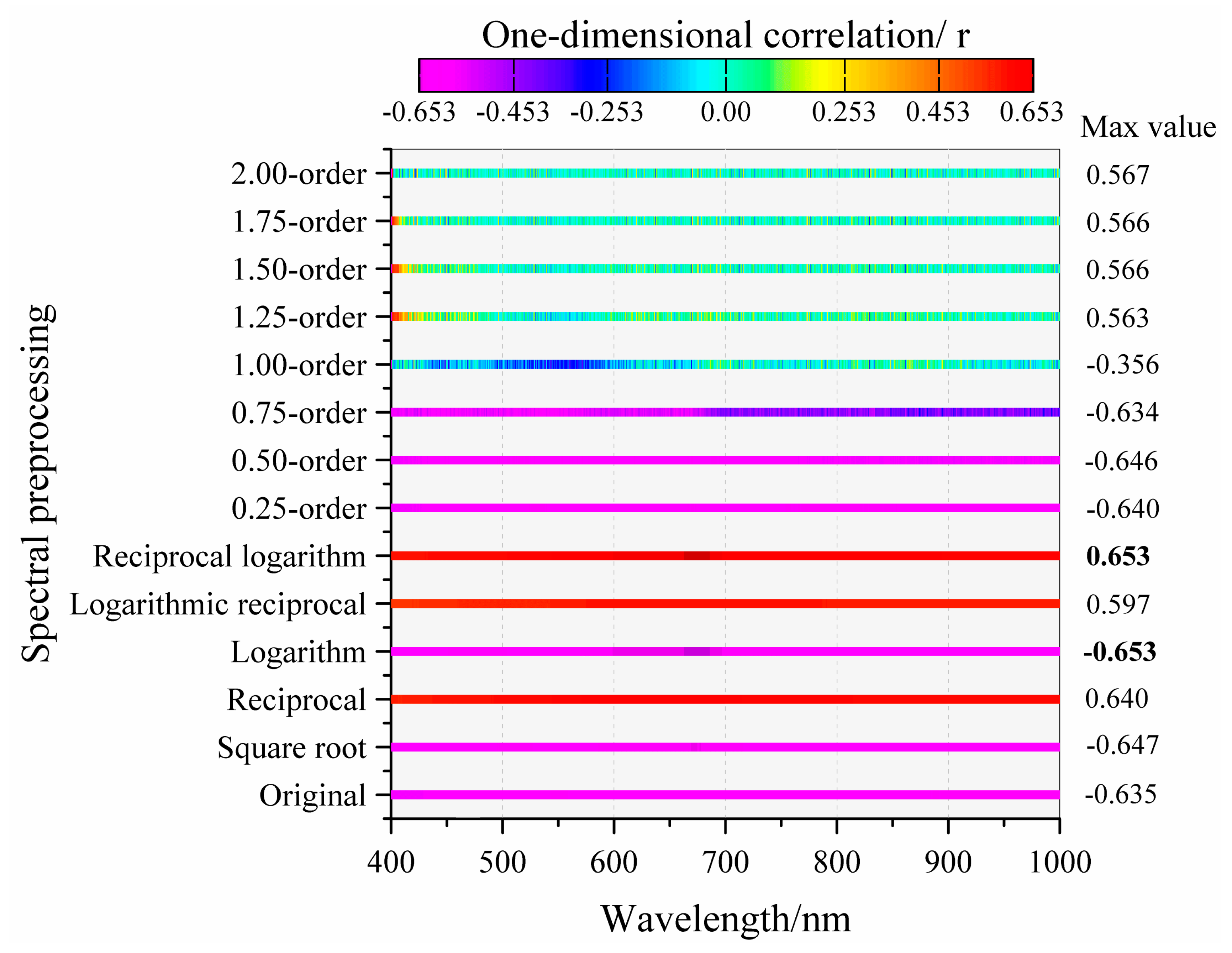
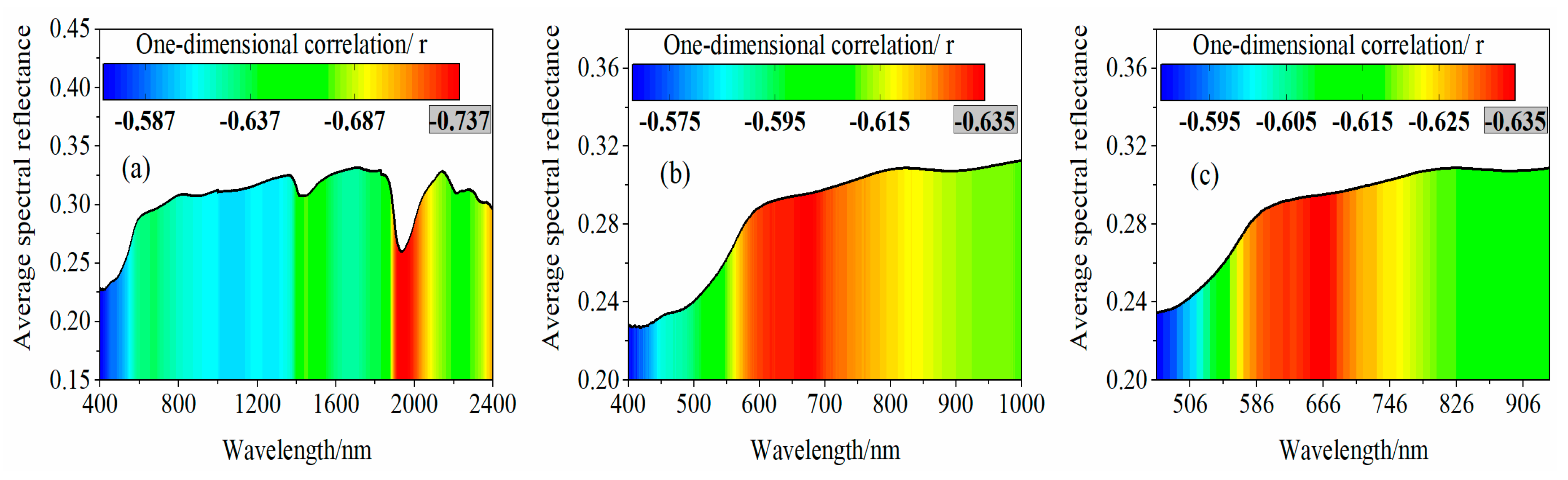
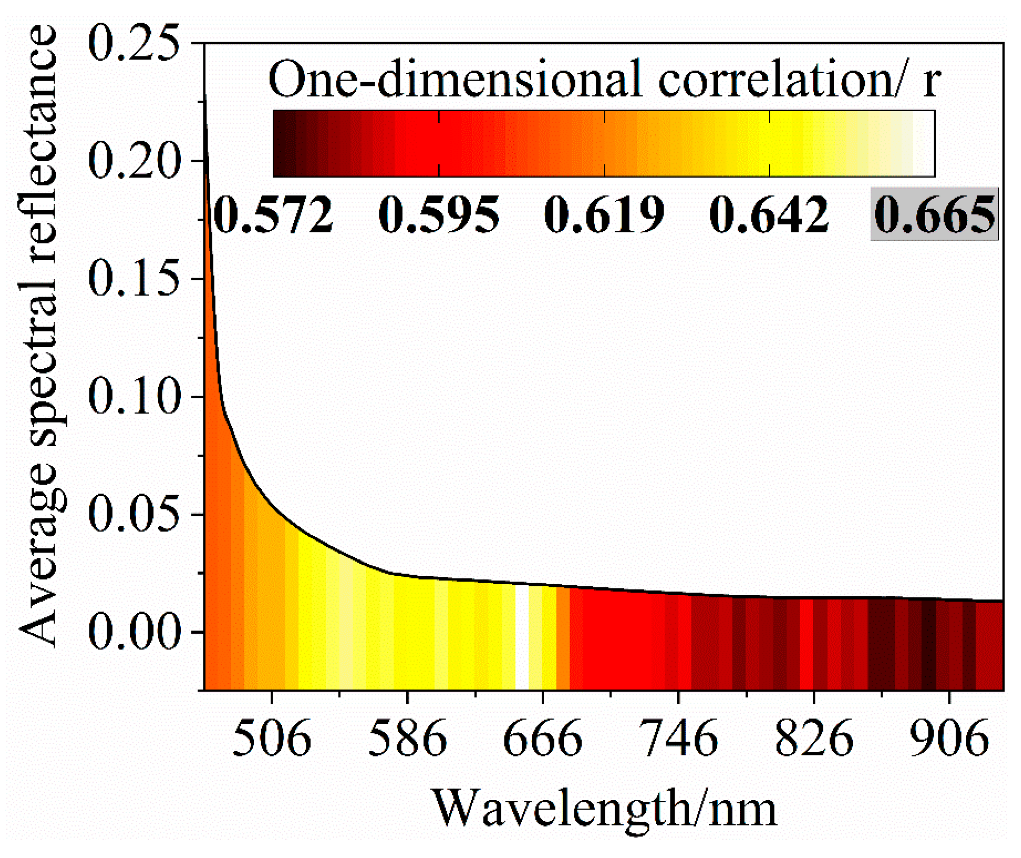
3.2.1. One-Dimensional PCC Analysis of SMC and Spectrum
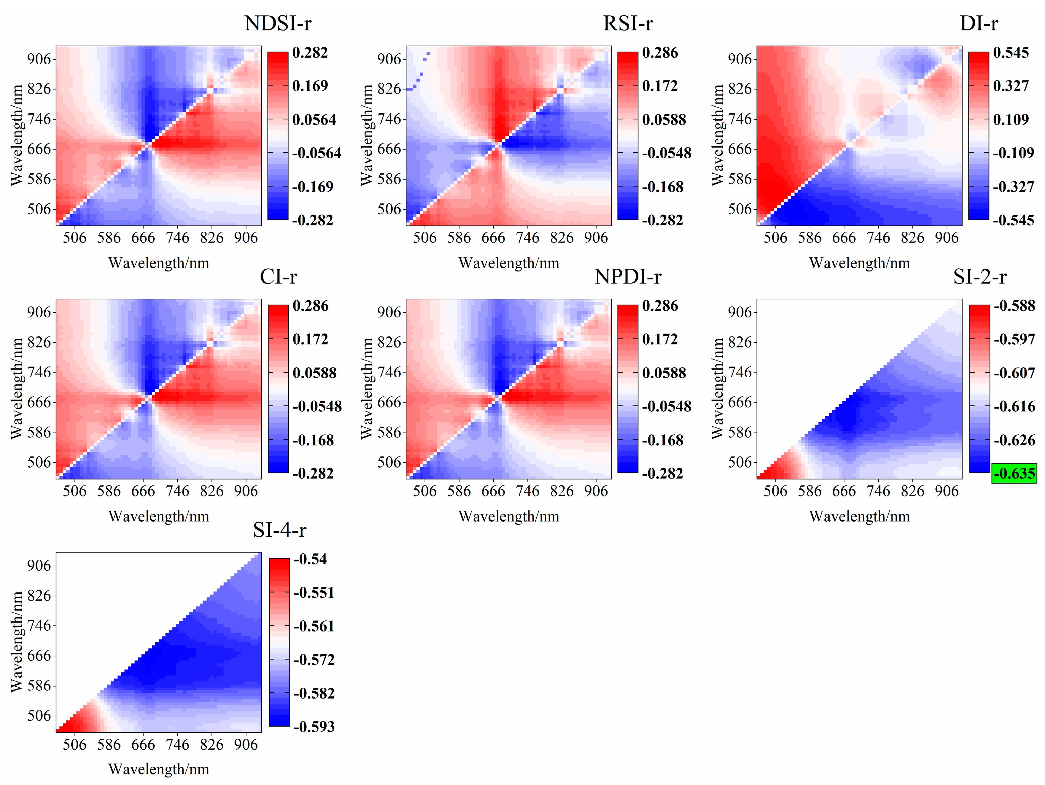
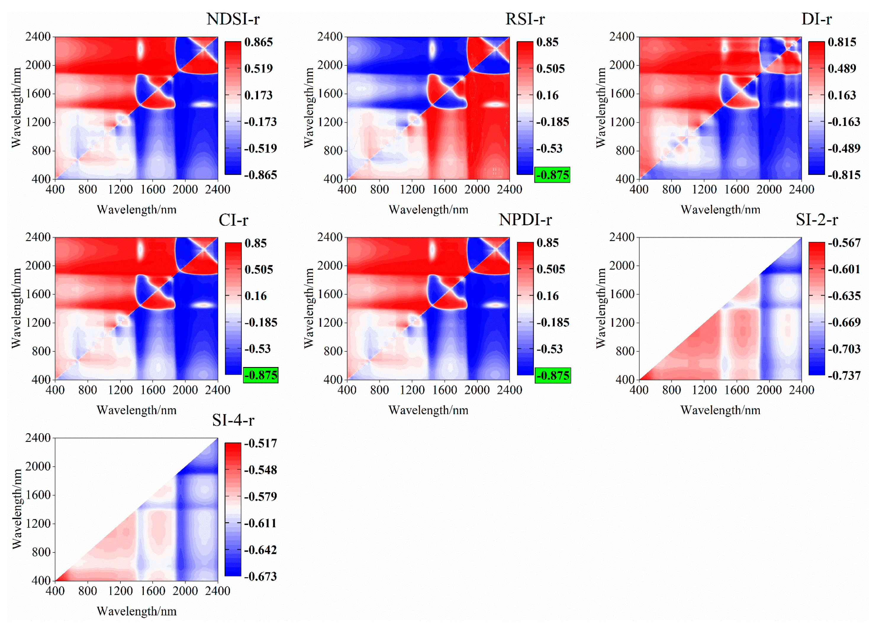
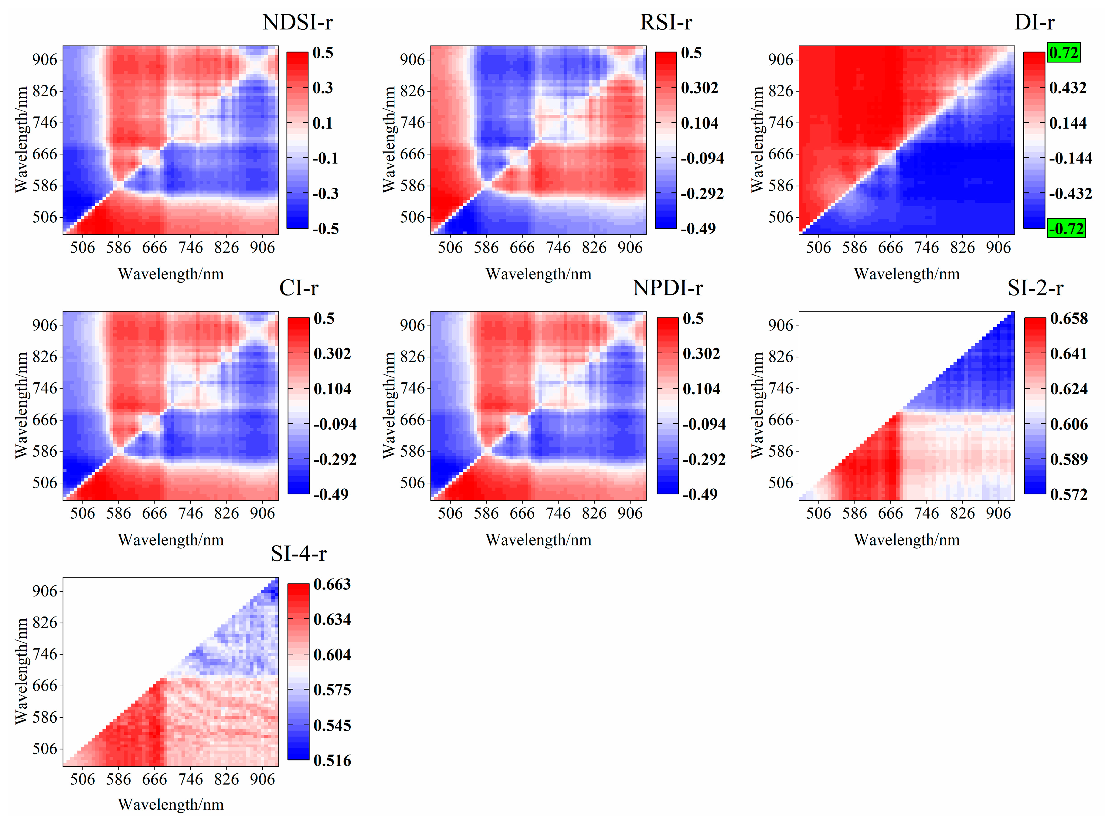
3.2.2. Two-Dimensional PCC Analysis of SMC and Spectrum
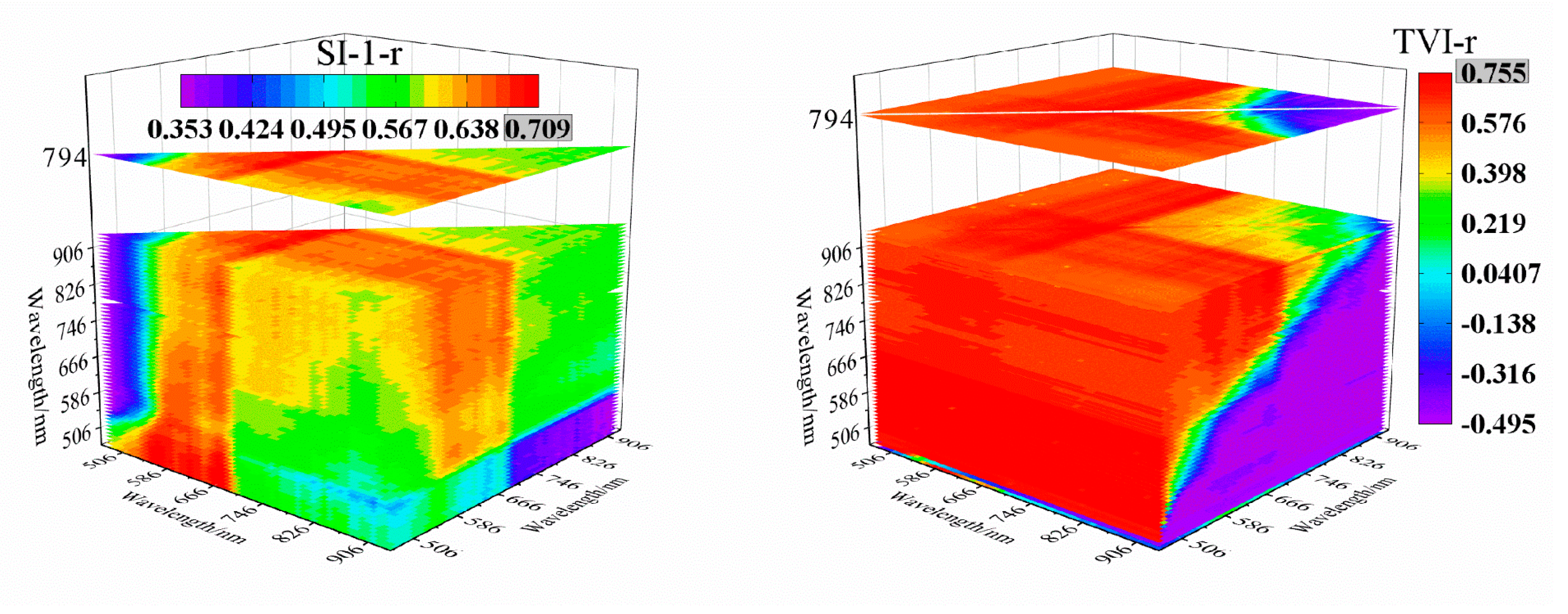
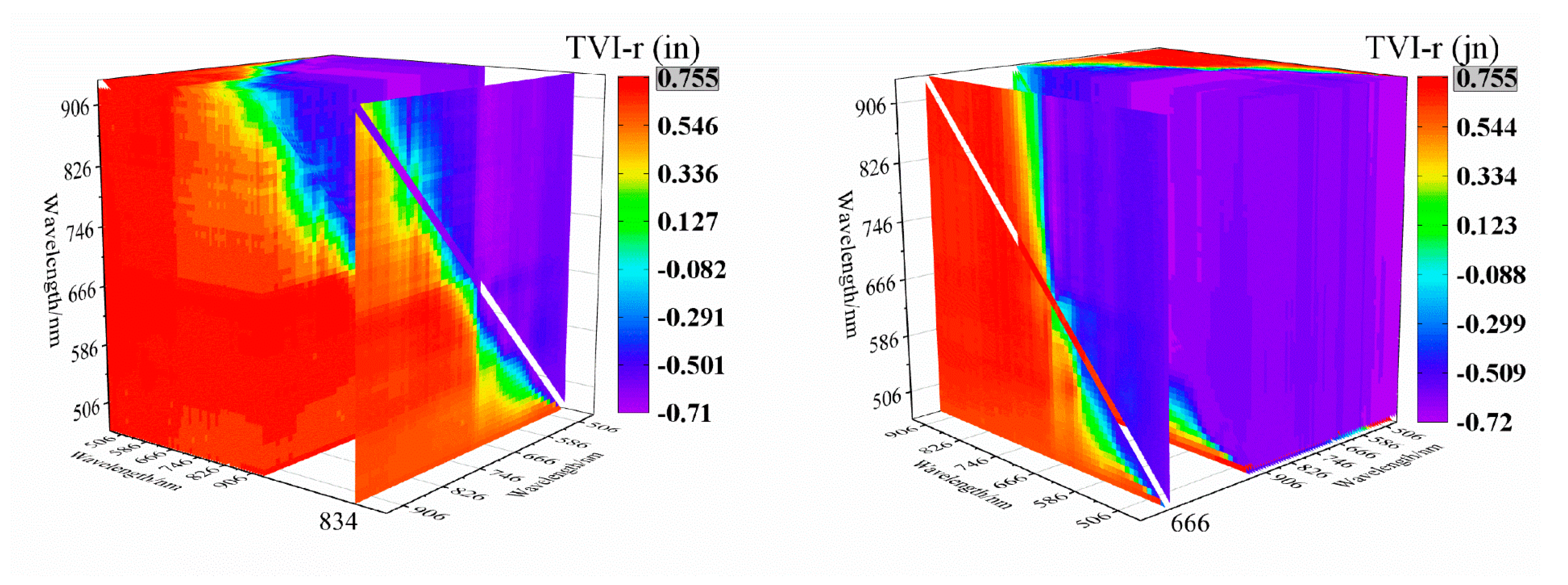
3.2.3. Three-Dimensional PCC Analysis of SMC and Spectrum
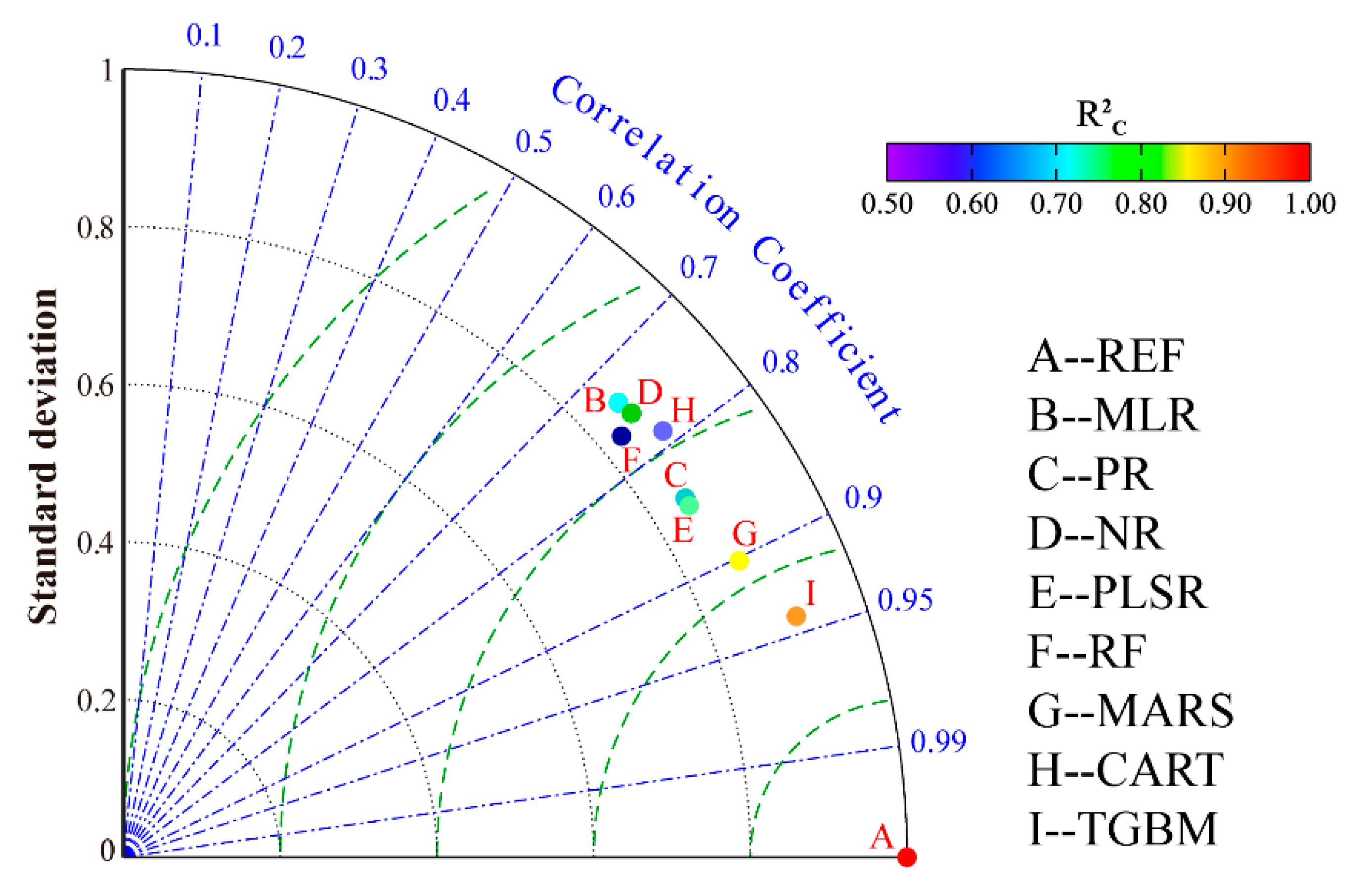
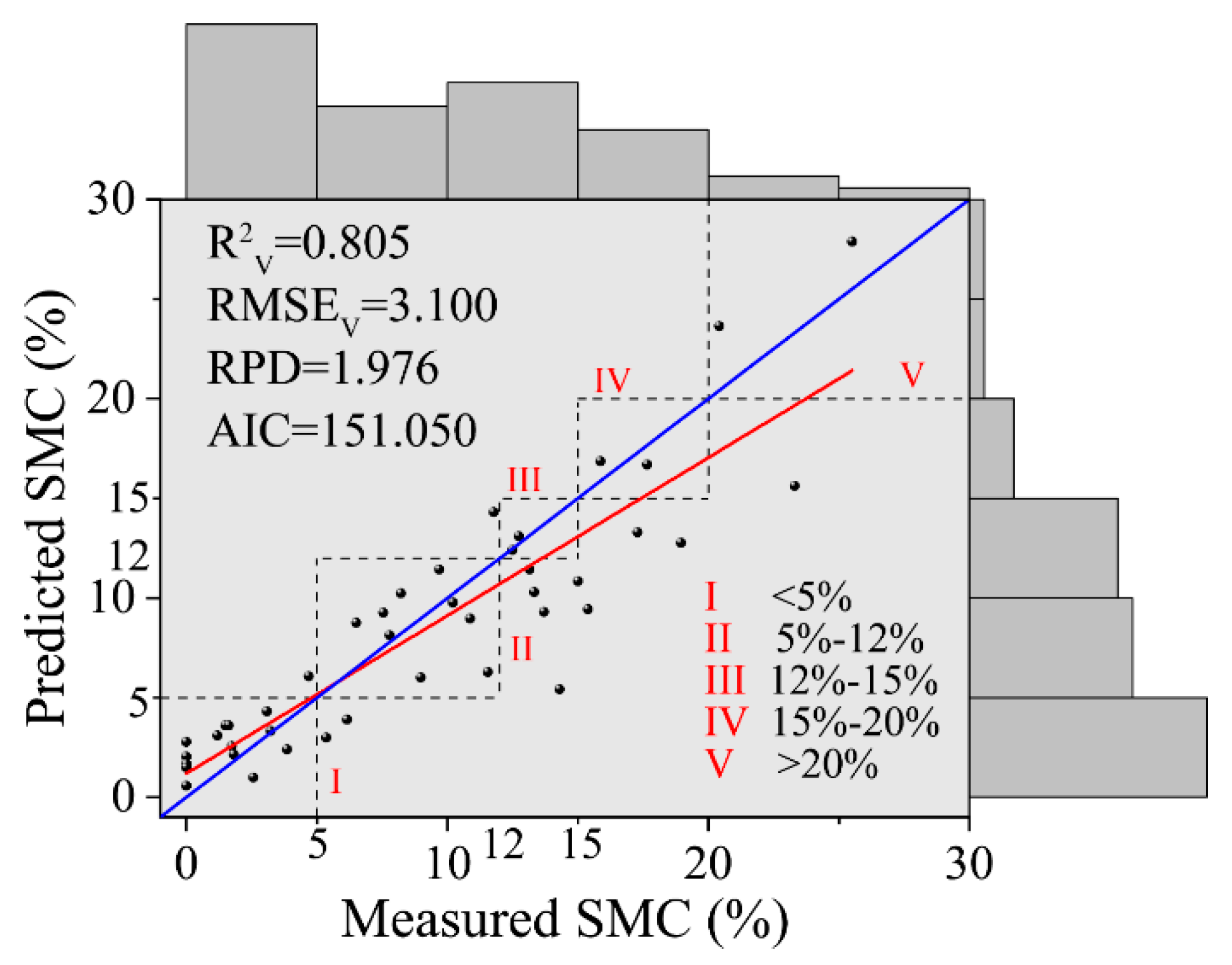
3.3. Model
4. Discussion
4.1. Discussion on Optimized Spectral Indices
4.2. Discussion on Fractional Order Differential
4.3. Discussion on Spectral Scale
4.4. Discussion on Models
4.5. Discussion on Zhuhai-1 Hyperspectral Imagery
5. Conclusions
Author Contributions
Funding
Acknowledgments
Conflicts of Interest
References
- Ebtehaj, A.; Bras, R.L. A physically constrained inversion for high-resolution passive microwave retrieval of soil moisture and vegetation water content in L-band. Remote Sens. Environ. 2019, 233, 111346. [Google Scholar] [CrossRef]
- Bablet, A.; Viallefont, F.; Jacquemoud, S.; Fabre, S.; Briottet, X. High-resolution mapping of in-depth soil moisture content through a laboratory experiment coupling a spectroradiometer and two hyperspectral cameras. Remote Sens. Environ. 2020, 236, 111533. [Google Scholar] [CrossRef]
- Aumann, H.H.; Chahine, M.T.; Gautier, C.; Goldberg, M.D.; Kalnay, E.; McMillin, L.M.; Revercomb, H.; Rosenkranz, P.W.; Smith, W.L.; Staelin, D.H.; et al. AIRS/AMSU/HSB on the Aqua mission: Design, science objectives, data products, and processing systems. IEEE Trans. Geosci. Remote Sens. 2003, 41, 253–264. [Google Scholar] [CrossRef] [Green Version]
- Chen, C. Science mapping: A systematic review of the literature. J. Data Inf. Sci. 2017, 2, 1–40. [Google Scholar] [CrossRef] [Green Version]
- Chen, C.; Hu, Z.; Liu, S.; Tseng, H. Emerging trends in regenerative medicine: A scientometric analysis in CiteSpace. Expert Opin. Biol. Ther. 2012, 12, 593–608. [Google Scholar] [CrossRef]
- Lu, P.; Wang, L.; Niu, Z.; Li, L.; Zhang, W. Prediction of soil properties using laboratory VIS–NIR spectroscopy and Hyperion imagery. J. Geochem. Explor. 2013, 132, 26–33. [Google Scholar] [CrossRef]
- Tiwari, S.K.; Saha, S.K.; Kumar, S. Prediction modeling and mapping of soil carbon content using artificial neural network, hyperspectral satellite data and field spectroscopy. Adv. Remote Sens. 2015, 4, 63–72. [Google Scholar] [CrossRef] [Green Version]
- Gomez, C.; Drost, A.; Roger, J. Analysis of the uncertainties affecting predictions of clay contents from VNIR/SWIR hyperspectral data. Remote Sens. Environ. 2015, 156, 58–70. [Google Scholar] [CrossRef] [Green Version]
- Gomez, C.; Gholizadeh, A.; Borůvka, L.; Lagacherie, P. Using legacy data for correction of soil surface clay content predicted from VNIR/SWIR hyperspectral airborne images. Geoderma 2016, 276, 84–92. [Google Scholar] [CrossRef]
- Gomez, C.; Oltra-Carrió, R.; Bacha, S.; Lagacherie, P.; Briottet, X. Evaluating the sensitivity of clay content prediction to atmospheric effects and degradation of image spatial resolution using Hyperspectral VNIR/SWIR imagery. Remote Sens. Environ. 2015, 164, 1–15. [Google Scholar] [CrossRef]
- Vaudour, E.; Gilliot, J.-M.; Bel, L.; Lefevre, J.; Chehdi, K. Regional prediction of soil organic carbon content over temperatecroplands using visible near-infrared airborne hyperspectral imageryand synchronous field spectra. Int. J. Appl. Earth Obs. Geoinf. 2016, 49, 24–38. [Google Scholar] [CrossRef]
- Ouerghemmi, W.; Gomez, C.; Naceur, S.; Lagacherie, P. Semi-blind source separation for the estimation of the clay content over semi-vegetated areas using VNIR/SWIR hyperspectral airborne data. Remote Sens. Environ. 2016, 181, 251–263. [Google Scholar] [CrossRef]
- Peón, J.; Recondo, C.; Fernández, S.; Calleja, J.J.F.; De Miguel, E.; Carretero, L. Prediction of Topsoil Organic Carbon Using Airborne and Satellite Hyperspectral Imagery. Remote Sens. 2017, 9, 1211. [Google Scholar] [CrossRef] [Green Version]
- Liu, L.; Ji, M.; Buchroithner, M.F. Transfer learning for soil spectroscopy based on convolutional neural networks and its application in soil clay content mapping using hyperspectral imagery. Sensors 2018, 18, 3169. [Google Scholar] [CrossRef] [PubMed] [Green Version]
- Ge, X.; Wang, J.; Ding, J.-L.; Cao, X.; Zhang, Z.; Liu, J.; Li, X. Combining UAV-based hyperspectral imagery and machine learning algorithms for soil moisture content monitoring. PeerJ 2019, 7, e6926. [Google Scholar] [CrossRef] [PubMed]
- Li, F.; Mistele, B.; Hu, Y.; Chen, X.; Schmidhalter, U. Optimising three-band spectral indices to assess aerial N concentration, N uptake and aboveground biomass of winter wheat remotely in China and Germany. ISPRS J. Photogramm. Remote Sens. 2014, 92, 112–123. [Google Scholar] [CrossRef]
- Wang, J.; Ding, J.; Yu, D.; Ma, X.; Zhang, Z.; Ge, X.; Teng, D.; Li, X.; Liang, J.; Lizaga, I.; et al. Capability of Sentinel-2 MSI data for monitoring and mapping of soil salinity in dry and wet seasons in the Ebinur Lake region, Xinjiang, China. Geoderma 2019, 353, 172–187. [Google Scholar] [CrossRef]
- Ainiwaer, M.; Ding, J.; Kasim, N.; Wang, J.; Wang, J. Regional scale soil moisture content estimation based on multi-source remote sensing parameters. Int. J. Remote Sens. 2019, 41, 3346–3367. [Google Scholar] [CrossRef]
- Liu, C.; Zhang, F.; Ge, X.; Zhang, X.; Chan, N.W.; Qi, Y. Measurement of total nitrogen concentration in surface water using hyperspectral band observation method. Water 2020, 12, 1842. [Google Scholar] [CrossRef]
- Kahaer, Y.; Shengtian, Y.; Tashpolat, N.; Fei, Z. Hyperspectral estimation of soil electrical conductivity based on fractional order differentially optimized spectral indices. Acta Ecol. Sin. 2019, 39, 7237–7248. [Google Scholar] [CrossRef]
- Zhang, Z.; Ding, J.-L.; Wang, J.; Ge, X. Prediction of soil organic matter in northwestern China using fractional order derivative spectroscopy and modified normalized difference indices. Catena 2020, 185. [Google Scholar] [CrossRef]
- Hong, Y.; Chen, S.; Zhang, Y.; Chen, Y.; Yu, L.; Liu, Y.; Liu, Y.; Cheng, H.; Liu, Y. Rapid identification of soil organic matter level via visible and near-infrared spectroscopy: Effects of two-dimensional correlation coefficient and extreme learning machine. Sci. Total. Environ. 2018, 644, 1232–1243. [Google Scholar] [CrossRef] [PubMed]
- Zhu, C.; Zhang, Z.; Wang, H.; Wang, J.; Yang, S. Assessing soil organic matter content in a coal mining area through spectral variables of different numbers of dimensions. Sensors 2020, 20, 1795. [Google Scholar] [CrossRef] [PubMed] [Green Version]
- Sawut, R.; Kasim, N.; Abliz, A.; Hu, L.; Yalkun, A.; Maihemuti, B.; Qingdong, S. Possibility of optimized indices for the assessment of heavy metal contents in soil around an open pit coal mine area. Int. J. Appl. Earth Obs. Geoinf. 2018, 73, 14–25. [Google Scholar] [CrossRef]
- Hong, Y.; Shen, R.; Cheng, H.; Chen, Y.; Zhang, Y.; Liu, Y.; Zhou, M.; Yu, L.; Liu, Y.; Liu, Y. Estimating lead and zinc concentrations in peri-urban agricultural soils through reflectance spectroscopy: Effects of fractional-order derivative and random forest. Sci. Total Environ 2019, 651, 1969–1982. [Google Scholar] [CrossRef]
- Wang, X.; Zhang, F.; Ding, J.; Kung, H.-T.; Latif, A.; Johnson, V.C. Estimation of soil salt content (SSC) in the Ebinur LakeWetland National Nature Reserve (ELWNNR), Northwest China, based on a Bootstrap-BP neural network model and optimal spectral indices. Sci. Total Environ. 2018, 615, 918–930. [Google Scholar] [CrossRef]
- Kahaer, Y.; Tashpolat, N. Estimating salt concentrations based on optimized spectral indices in soils with regional heterogeneity. J. Spectrosc. 2019. [Google Scholar] [CrossRef]
- Li, C.; Zhang, G.-W.; Zhou, Z.; Zhao, W.-Q.; Meng, Y.-L.; Chen, B.; Wang, Y. Hyperspectral parameters and prediction model of soil moisture in coastal saline. Chin. J. Appl. Ecol. 2016, 27, 525–531. [Google Scholar] [CrossRef]
- Wang, X.; Zhang, F.; Kung, H.-T.; Johnson, V.C. New methods for improving the remote sensing estimation of soil organic matter content (SOMC) in the Ebinur Lake Wetland National Nature Reserve (ELWNNR) in northwest China. Remote Sens. Environ. 2018, 218, 104–118. [Google Scholar] [CrossRef]
- Jingzhe, W.; Jianli, D.; Xuankai, M.; Xiangyu, G.; Bohua, L.; Jing, L. Detection of soil moisture content based on UAV-derived hyperspectral imagery and spectral index in oasis cropland. Trans. Chin. Soc. Agric. Mach. 2018, 49, 164–172. [Google Scholar] [CrossRef]
- Xianlong, Z.; Fei, Z.; Haiwei, Z.; Zhe, L.; Qing, H.; Lihua, C. Optimization of soil salt inversion model based on spectral transformation from hyperspectral index. Trans. Chin. Soc. Agric. Eng. 2018, 34, 110–117. [Google Scholar] [CrossRef]
- Kasim, N.; Maihemuti, B.; Sawut, R.; Abliz, A.; Cui, D.; Abdumutallip, M. Quantitative estimation of soil salinization in an arid region of the Keriya Oasis based on multidimensional modeling. Water 2020, 12, 880. [Google Scholar] [CrossRef] [Green Version]
- Xu, C.; Zeng, W.; Huang, J.; Wu, J.; van Leeuwen, W.J.D. Prediction of soil moisture content and soil salt concentration from hyperspectral laboratory and field data. Remote Sens. 2016, 8, 42. [Google Scholar] [CrossRef] [Green Version]
- Oltra-Carrió, R.; Baup, F.; Fabre, S.; Fieuzal, R.; Briottet, X. Improvement of soil moisture retrieval from hyperspectral VNIR-SWIR data using clay content information: From laboratory to field experiments. Remote Sens. 2015, 7, 3184–3205. [Google Scholar] [CrossRef] [Green Version]
- Yue, J.; Tian, J.; Tian, Q.; Xu, K.; Xu, N. Development of soil moisture indices from differences in water absorption between shortwave-infrared bands. ISPRS J. Photogramm. Remote Sens. 2019, 154, 216–230. [Google Scholar] [CrossRef]
- Zhang, Y.; Tan, K.; Wang, X.; Chen, Y. Retrieval of soil moisture content based on a modified Hapke photometric model: A novel method applied to laboratory hyperspectral and Sentinel-2 MSI data. Remote Sens. 2020, 12, 2239. [Google Scholar] [CrossRef]
- Haubrock, S.-N.; Kuhnert, M.; Hostert, P.; Kaufmann, H.; Chabrillat, S. Surface soil moisture quantification and validation based on hyperspectral data and field measurements. J. Appl. Remote Sens. 2008, 2, 023552. [Google Scholar] [CrossRef] [Green Version]
- Schlerf, M.; Atzberger, C. Inversion of a forest reflectance model to estimate structural canopy variables from hyperspectral remote sensing data. Sens. Environ. 2006, 100, 281–294. [Google Scholar] [CrossRef]
- Yuan, H.; Yang, G.; Li, C.; Wang, Y.; Liu, J.; Yu, H.; Feng, H.; Xu, B.; Zhao, X.; Yang, X. Retrieving soybean leaf area index from unmanned aerial vehicle hyperspectral remote sensing: Analysis of RF, ANN, and SVM regression models. Remote Sens. 2017, 9, 309. [Google Scholar] [CrossRef] [Green Version]
- Lagacherie, P.; Arrouays, D.; Bourennane, H.; Gomez, C.; Martin, M.; Saby, N.P. How far can the uncertainty on a Digital Soil Map be known? A numerical experiment using pseudo values of clay content obtained from Vis-SWIR hyperspectral imagery. Geoderma 2019, 337, 1320–1328. [Google Scholar] [CrossRef]
- Ainiwaer, M.; Ding, J.-L.; Wang, J.; Nasierding, N. Spatiotemporal dynamics of water table depth associated with changing agricultural land use in an arid zone oasis. Water 2019, 11, 673. [Google Scholar] [CrossRef] [Green Version]
- Huang, S.; Ding, J.-L.; Liu, B.; Ge, X.; Wang, J.; Zou, J.; Zhang, J. The Capability of integrating optical and microwave data for detecting soil moisture in an oasis region. Remote Sens. 2020, 12, 1358. [Google Scholar] [CrossRef]
- Huang, S.; Ding, J.-L.; Zou, J.; Liu, B.; Zhang, J.; Chen, W. Soil Moisture Retrival Based on Sentinel-1 Imagery under Sparse Vegetation Coverage. Sensors 2019, 19, 589. [Google Scholar] [CrossRef] [PubMed] [Green Version]
- Tashpolat, N.; Ding, J.-L.; Yu, D. Dielectric properties of saline soil based on a modified Dobson dielectric model. J. Arid. Land 2015, 7, 696–705. [Google Scholar] [CrossRef] [Green Version]
- Wang, F.; Shi, Z.; Biswas, A.; Yang, S.; Ding, J. Multi-algorithm comparison for predicting soil salinity. Geoderma 2020, 365, 114211. [Google Scholar] [CrossRef]
- Jiang, Y.; Wang, J.; Zhang, L.; Zhang, G.; Li, X.; Wu, J. Geometric processing and accuracy verification of Zhuhai-1 hyperspectral satellites. Remote Sens. 2019, 11, 996. [Google Scholar] [CrossRef] [Green Version]
- Huadong, G.; Guang, L.; Dong, L.; Lu, Z.; Han, X. Progress of Earth observation in China. Chin. J. Space Sci. 2018, 38, 797–809. [Google Scholar] [CrossRef]
- Yépez-Martínez, H.; Gómez-Aguilar, J. A new modified definition of Caputo-Fabrizio fractional-order derivative and their applications to the Multi Step Homotopy Analysis Method. J. Comput. Appl. Math. 2018. [Google Scholar] [CrossRef]
- Hong, Y.; Chen, S.; Liu, Y.; Zhang, Y.; Yu, L.; Chen, Y.; Liu, Y.; Cheng, H.; Liu, Y. Combination of fractional order derivative and memory-based learning algorithm to improve the estimation accuracy of soil organic matter by visible and near-infrared spectroscopy. Catena 2019, 174, 104–116. [Google Scholar] [CrossRef]
- Hong, Y.; Liu, Y.; Chen, Y.; Liu, Y.; Yu, L.; Liu, Y.; Cheng, H. Application of fractional-order derivative in the quantitative estimation of soil organic matter content through visible and near-infrared spectroscopy. Geoderma 2019, 337, 758–769. [Google Scholar] [CrossRef]
- Chen, X.; Huang, J.; Yi, M. Cost estimation for general aviation aircrafts using regression models and variable importance in projection analysis. J. Clean. Prod. 2020, 256, 120648. [Google Scholar] [CrossRef]
- Mullet, T.C.; Gage, S.H.; Morton, J.M.; Huettmann, F. Temporal and spatial variation of a winter soundscape in south-central Alaska. Landsc. Ecol. 2016, 31, 1117–1137. [Google Scholar] [CrossRef]
- Suon, S.; Li, Y.; Porn, L.; Javed, T. Spatiotemporal Analysis of Soil Moisture Drought over China during 2008–2016. J. Water Resour. Prot. 2019, 11, 700–712. [Google Scholar] [CrossRef] [Green Version]
- Pôças, I.; Calera, A.; Campos, I.; Cunha, M. Remote sensing for estimating and mapping single and basal crop coefficientes: A review on spectral vegetation indices approaches. Agric. Water Manag. 2020, 233, 106081. [Google Scholar] [CrossRef]
- Wang, J.; Ding, J.; Abulimiti, A.; Cai, L. Quantitative estimation of soil salinity by means of different modeling methods and visble-near infrared (VIS-NIR) spectroscopy, Ebinur Lake Wetland, Northwest China. PeerJ 2018, 6, e4703. [Google Scholar] [CrossRef] [PubMed] [Green Version]
- Du, H.; Jiang, H.; Zhang, L.; Mao, D.; Wang, Z. Evaluation of spectral scale effects in estimation of vegetation leaf area index using spectral indices methods. Chin. Geogr. Sci. 2016, 26, 731–744. [Google Scholar] [CrossRef] [Green Version]
- Sims, D.A.; Gamon, J.A. Relationships between leaf pigment content and spectral reflectance across a wide range of species, leaf structures and developmental stages. Remote Sens. Environ. 2002, 81, 337–354. [Google Scholar] [CrossRef]


| Channel | Center | Channel | Center | Channel | Center | Channel | Center |
|---|---|---|---|---|---|---|---|
| B01 | 466 | B09 | 596 | B17 | 716 | B25 | 836 |
| B02 | 480 | B10 | 610 | B18 | 730 | B26 | 850 |
| B03 | 500 | B11 | 626 | B19 | 746 | B27 | 866 |
| B04 | 520 | B12 | 640 | B20 | 760 | B28 | 880 |
| B05 | 536 | B13 | 656 | B21 | 776 | B29 | 896 |
| B06 | 550 | B14 | 670 | B22 | 790 | B30 | 910 |
| B07 | 566 | B15 | 686 | B23 | 806 | B31 | 926 |
| B08 | 580 | B16 | 700 | B24 | 820 | B32 | 940 |
| Channel | Center | Channel | Center | Channel | Center | Channel | Center |
|---|---|---|---|---|---|---|---|
| B01 | 466 | B16 | 586 | B31 | 706 | B46 | 826 |
| B02 | 474 | B17 | 594 | B32 | 714 | B47 | 834 |
| B03 | 482 | B18 | 602 | B33 | 722 | B48 | 842 |
| B04 | 490 | B19 | 610 | B34 | 730 | B49 | 850 |
| B05 | 498 | B20 | 618 | B35 | 738 | B50 | 858 |
| B06 | 506 | B21 | 626 | B36 | 746 | B51 | 866 |
| B07 | 514 | B22 | 634 | B37 | 754 | B52 | 874 |
| B08 | 522 | B23 | 642 | B38 | 762 | B53 | 882 |
| B09 | 530 | B24 | 650 | B39 | 770 | B54 | 890 |
| B10 | 538 | B25 | 658 | B40 | 778 | B55 | 898 |
| B11 | 546 | B26 | 666 | B41 | 786 | B56 | 906 |
| B12 | 554 | B27 | 674 | B42 | 794 | B57 | 914 |
| B13 | 562 | B28 | 682 | B43 | 802 | B58 | 922 |
| B14 | 570 | B29 | 690 | B44 | 810 | B59 | 930 |
| B15 | 578 | B30 | 698 | B45 | 818 | B60 | 938 |
| Degree of Drought | SMC |
|---|---|
| High humidity | >20% |
| Suitable humidity | 15–20% |
| Mild drought | 12–15% |
| Moderate drought | 5–12% |
| Severe drought | <5% |
| Model | R2V | RMSEV (%) | RPD |
|---|---|---|---|
| MLR | 0.694 | 3.181 | 1.888 |
| PR | 0.684 | 3.870 | 1.495 |
| NR | 0.726 | 3.631 | 1.518 |
| PLSR | 0.787 | 3.247 | 2.071 |
| RF | 0.662 | 3.771 | 1.744 |
| MARS | 0.774 | 3.084 | 1.972 |
| CART | 0.544 | 4.922 | 1.245 |
| TGBM | 0.707 | 3.525 | 1.879 |
| Number of Variables | R2C | RMSEC (%) | R2V | RMSEV (%) |
|---|---|---|---|---|
| 54 | 0.727 | 3.061 | 0.796 | 2.545 |
| 27 | 0.733 | 3.028 | 0.805 | 3.100 |
| 9 | 0.738 | 3.002 | 0.761 | 2.627 |
Publisher’s Note: MDPI stays neutral with regard to jurisdictional claims in published maps and institutional affiliations. |
© 2020 by the authors. Licensee MDPI, Basel, Switzerland. This article is an open access article distributed under the terms and conditions of the Creative Commons Attribution (CC BY) license (http://creativecommons.org/licenses/by/4.0/).
Share and Cite
Kahaer, Y.; Tashpolat, N.; Shi, Q.; Liu, S. Possibility of Zhuhai-1 Hyperspectral Imagery for Monitoring Salinized Soil Moisture Content Using Fractional Order Differentially Optimized Spectral Indices. Water 2020, 12, 3360. https://doi.org/10.3390/w12123360
Kahaer Y, Tashpolat N, Shi Q, Liu S. Possibility of Zhuhai-1 Hyperspectral Imagery for Monitoring Salinized Soil Moisture Content Using Fractional Order Differentially Optimized Spectral Indices. Water. 2020; 12(12):3360. https://doi.org/10.3390/w12123360
Chicago/Turabian StyleKahaer, Yasenjiang, Nigara Tashpolat, Qingdong Shi, and Suhong Liu. 2020. "Possibility of Zhuhai-1 Hyperspectral Imagery for Monitoring Salinized Soil Moisture Content Using Fractional Order Differentially Optimized Spectral Indices" Water 12, no. 12: 3360. https://doi.org/10.3390/w12123360
APA StyleKahaer, Y., Tashpolat, N., Shi, Q., & Liu, S. (2020). Possibility of Zhuhai-1 Hyperspectral Imagery for Monitoring Salinized Soil Moisture Content Using Fractional Order Differentially Optimized Spectral Indices. Water, 12(12), 3360. https://doi.org/10.3390/w12123360