Article

A Novel Hybrid Approach for Water Resources Carrying Capacity Assessment by Integrating Fuzzy Comprehensive Evaluation and Analytical Hierarchy Process Methods with the Cloud Model

1
School of Civil and Hydraulic Engineering, Huazhong University of Science and Technology, Wuhan 430074, China
2
Hydrology and Water Resources Survey Station of Shanxi Province, Taiyuan 030001, China
3
College of Data Science, Taiyuan University of Technology, Taiyuan 030024, China
4
Changjiang Institute of Survey, Planning, Design and Research, Wuhan 430000, China
*
Author to whom correspondence should be addressed.
Water 2020, 12(11), 3241; https://doi.org/10.3390/w12113241
Submission received: 6 September 2020 / Revised: 12 November 2020 / Accepted: 17 November 2020 / Published: 19 November 2020
(This article belongs to the Section Water Resources Management, Policy and Governance)

Abstract

:
The water resources carrying capacity (WRCC) shows remarkable fuzziness and randomness, which causes the uncertainty and instability of the WRCC assessment (WRCCA). In order to solve these problems, we proposed a novel hybrid approach for WRCCA, in which the fuzzy comprehensive evaluation (FCE) and analytical hierarchy process (AHP) methods were integrated with the cloud model (CM). Firstly, an evaluation indicator system of WRCC was constructed. Secondly, the AHP and FCE methods were subsequently improved with the CM. The CM was used to scale the relative importance and aggregate the judgment matrices, where the weights of the clouds were obtained. These integrations of AHP and CM greatly reduced the randomness in the weight calculation; the CM was used to describe the comment sets, calculate the membership degree matrices and determine the assignment clouds, the evaluation sets and the WRCCA index clouds were obtained. These integrations of FCE and CM effectively blurred the boundary fuzziness and gave more intuitive results. Finally, the hybrid FCE-AHP-CM approach was applied to a case study. It was concluded that the novel approach has particular advantages in dealing with the fuzziness and randomness comprehensively, and therefore could assess the WRCC and enhance the robustness and intuition of WRCCA results.

1. Introduction

Water resources play crucial roles in human civilization, social and economic development, ecological environment, and so on. Conversely, the water resources carrying capacity (WRCC) in a region is the decisive factor to its sustainable development. So, water resources carrying capacity assessment (WRCCA) is always a very important research topic in the fields of hydrology, water resources management and socio-economic sustainable development [1].
WRCC is the specific application of the carrying capacity concept in the field of water resources. In 1921, Park et al. initially introduced the concept of carrying capacity into human ecology [2], and in 1985, the definition of resources carrying capacity was proposed by the United Nations Educational, Scientific and Cultural Organization [3]. Since the concept of sustainable development was put forward, the researches on WRCC continued to appear. The URS company in the United States defined the WRCC as the maximum level of development that a region’s water resources can carry without destroying natural and artificial resources [4]. In China, the Xinjiang Water Resources Soft Science Research Group firstly proposed the concept of WRCC in 1989 [5]. The understanding of WRCC can be summarized in three perspectives such as the maximum development, supporting, and carrying capacity of water resources [6,7,8,9,10].
The WRCCA can be roughly divided into two categories. One is the largest economic and social development scale that water resources can carry, and the other is the maximum carrying capacity of water resources to the existing economic and social development scale. The carrying scale is usually evaluated by system dynamics, conventional trend, and multi-objective analysis methods [11,12], while the carrying capacity is usually evaluated by principal component analysis (PCA), projection pursuit evaluation, analytical hierarchy process (AHP), fuzzy comprehensive evaluation (FCE), neural network, and machine learning methods [13,14,15]. The establishment of an evaluation indicator system is the first step for WRCCA. There are usually two methods used to construct the evaluation indicator system. One is to divide the water resources system into different levels of subsystems which consist of different indicator elements, and these indicators are interconnected or independent from each other by tapping their meanings based on the expert advice [16]. The other is to select indicators according to the fixed-mode of Driving Force-Pressure-State-Impact-Response-Management (DPSIRM) [15,17,18,19,20].
It has been found that the influencing factors of WRCC are various and the process of WRCCA is complex. As a result, it is difficult to use a single model to evaluate the WRCC, and the combination of different models has become popular. Yang et al. combined the AHP with a system dynamics model to construct a multi-standard WRCCA indicators system and a socio-economic water resource dynamics model [21]. Chi et al. assessed the WRCC through AHP and FCE methods [22]. Dai et al. evaluated the WRCC by a water ecological footprint model combined with a system dynamics model [23]. Wu et al. proposed a comprehensive modeling framework by combining Soil and Water Assessment Tool (SWAT) model, water supply and demand model, PCA and FCE methods [24]. Ma et al. evaluated the regional WRCC based on set pair analysis and entropy weight methods [25].
According to the above analyses, it can be seen that a lot of researches on WRCCA have been conducted and great achievements have been made. However, there are still some limitations that need to be improved. Firstly, the evaluation indicator system construction of WRCC was seldom considered from the perspectives of water resource constraint conditions and optimization goals. The previous researches mainly focused on the exploitable scale or the ability of water resources so as to support the ecological environment and economic development, and therefore they only considered the influencing factors of water resources, economy, society, and environment. Secondly, WRCCA is a problem with multi-level and multi-indicator uncertainties like fuzziness and randomness, and such uncertainties have rarely been quantitatively described. Most studies employed experts’ subjective opinions to obtain the WRCCA results which are usually qualitative conclusions or single values. Thirdly, because of the complexity, fuzziness, and randomness of WRCCA, the evaluation models and methods have evolved from a single to combined approach. However, the advantages of different models and methods are rarely integrated together so as to achieve mutual improvements. Therefore, their simple combinations cannot yet well describe the fuzziness and randomness in the process of WRCCA.
In this paper, based on the fact that the entire water resources system is sensitive to the changes of hydrological conditions, especially in arid and semiarid regions, we constructed four subsystems for WRCCA, such as hydrology, water resources utilization, water ecological environment, and economy and society, in which the former two are constraints and the latter two are optimization objectives. On this basis, evaluation indicators were screened to improve the rationality and comprehensiveness of impact factors determination for WRCCA. Then, according to the principles of FCE and AHP methods as well as their combinations, we integrated them with the cloud model (CM) so as to consider both the fuzziness and randomness in WRCCA. Finally, the proposed AHP-FCE-CM hybrid approach for WRCCA was applied and validated in a case study—Datong City of Shanxi Province in North China.

2. Methodology

2.1. The Establishment Method of an Indicator-Based System for WRCCA

2.1.1. Selection of the Evaluation Indicator

In this paper, the WRCCA rules with hydrology and water resources utilization were used as constraints, and a virtuous cycle of water ecological environment and sustainable economic and social development as optimization goals were determined for arid and semiarid areas like North China. Therefore, the indicator system for WRCCA was firstly divided into 4 subsystems, such as hydrology, water resources utilization, water ecological environment, and economy and society. Then for each subsystem, the text matching method was used to select the evaluation indicators, the Spearman rank correlation analysis method was used to analyze the correlations between the indicators, and the gray correlation method was used to screen the indicators.
The text matching method selects indicators by querying the authoritative academic databases, such as Springer, Elsevier, and China National Knowledge Internet. The term of ‘water resources carrying capacity’ was firstly used as a key word for searching. After obtaining relevant matching documents, the key words of ‘evaluation indicator’ is entered again for screening. By counting the appearance number of each evaluation indicator, the ones with higher frequency are selected as the initial indicators.
The Spearman rank correlation analysis method was used to calculate the correlation coefficient between evaluation indicators, which helped to eliminate the redundant and highly relevant indicators, as well as the impacts of repeated information between indicators, and thereby simplified the evaluation indicator system. The calculation process is summarized as follows.
Assume that indicators X and Y have n sample values, Ri is the rank of Xi in (X1, X2, …, Xn), Qi is the rank of Yi in (Y1, Y2, …, Yn), then the rank correlation coefficient r X Y between indicators X and Y is defined as:
r X Y = i = 1 n [ ( R i 1 n i = 1 n R i ) ( Q i 1 n i = 1 n Q i ) ] i = 1 n ( R i 1 n i = 1 n R i ) 2 i = 1 n ( Q i 1 n i = 1 n Q i ) 2
Equation (1) can be further simplified as:
r X Y = 1 6 n ( n 2 1 ) i = 1 n ( R i Q i ) 2
Finally, the indicators with an absolute value of correlation coefficient greater than 0.9 are defined as repeated indicators, and only one of them is retained.
The gray correlation method was used to calculate and sort the average values of correlation coefficients between each indicator and other indicators, and thereby select the indicators that have relatively large impacts on the evaluation results. The steps shown as follows:
(1)
Determine the reference sequence
The serial values of one of the evaluation indicators are taken as the reference sequence, which are recorded as:
X 0 = ( x 0 ( 1 ) , x 0 ( 2 ) , , x 0 ( n ) ) T
where n is the number of evaluation areas.
(2)
Determine the comparison sequence
The indicator sequences other than reference sequences are used as comparison sequences, which are recorded as:
( X 1 , X 2 , , X m ) = [ x 1 ( 1 ) x 2 ( 1 ) x m ( 1 ) x 1 ( 2 ) x 2 ( 2 ) x m ( 2 ) x 1 ( n ) x 2 ( n ) x m ( n ) ]
where m is the number of evaluation indicators other than the reference indicator; X i = ( x i ( 1 ) , x i ( 2 ) , , x i ( n ) ) T ( i = 1 , 2 , , m ) .
(3)
Normalization of data sequence
The extreme value change method is used to perform normalization of the reference sequence and comparison sequence data, and the calculation formula is:
x k = x k m i n x k m a x x k m i n x k
where x k is the data after being rescaled; k is the evaluation indicator (k = 0, 1, …, m); min x k and max x k are the minimum and maximum values of the evaluation indicator k in all evaluation areas, respectively.
(4)
Calculate the absolute difference
The absolute difference between the reference sequence and the comparison sequence is calculated. That is, Δ k ( i ) = | x 0 ( i ) x k ( i ) | ( k = 1 , 2 , , m ) . Thus, the absolute difference matrix is:
| Δ 1 ( 1 ) Δ 2 ( 1 ) Δ m ( 1 ) Δ 1 ( 2 ) Δ 2 ( 2 ) Δ m ( 2 ) Δ 1 ( n ) Δ 2 ( n ) Δ m ( n ) |
(5)
Calculate the gray correlation coefficient
Equation (7) was adopted to calculate the gray correlation coefficient between each comparison sequence and the reference sequence.
α k ( i ) = min k min i Δ k ( i ) + β max k max i Δ k ( i ) Δ k ( i ) + β max k max i Δ k ( i )
where α k ( i ) is the gray correlation coefficient; Δ k ( i ) is the absolute difference between the indicator k sequence and the reference indicator sequence; min k min i Δ k ( i ) and max k max i Δ k ( i ) are the minimum and maximum values of the absolute difference, respectively. β (0 < β < 1) is the resolution ratio. The smaller the β is, the larger difference of correlation coefficient is and the stronger resolution is. Generally, β = 0.5.
(6)
Calculate the gray correlation degree
The gray correlation coefficients between the comparison sequence and reference sequence are calculated and averaged for all evaluation areas to obtain the grey correlation degree, which is described as:
g k = 1 n i = 1 n α k ( i )
In the same way, the reference sequence is changed in turn, and the correlation degrees between all indicators are calculated to obtain the correlation matrix. Each row of the correlation matrix is averaged, and the average value is the correlation degree value of the evaluation indicator to be filtered.
(7)
Sort the gray correlation degrees
The larger the correlation degree value in the calculation results, the closer the relationship between the comparison sequence and the reference sequence is. An indicator with a larger correlation degree value is selected as the evaluation indicator.

2.1.2. Determination of the Evaluation Indicator Criteria

According to the above qualitative, correlation and quantitative analysis, the evaluation indicators were screened. Based on their actual data structures, the data series of the study area were evenly divided, and the evaluation standards for different indicators were divided into different levels. Assume the data series of an indicator I is { I 1 , I 2 , , I n } and this indicator is divided into m levels, then:
(1)
The length ( L of the data sequence interval is calculated as:
L = max I min I
where max I and min I are the maximum and minimum of indicator I in the data series, respectively.
(2)
The average interval ( i ) of the data series is calculated as:
i = L / m = ( max I min I ) / m
(3)
Calculate the upper and lower limits of each level to obtain its interval; the m -th level I m I m can be expressed as:
I m = [ min I + ( m 1 ) i , min I + m i ]
By using this method, the level standards of each evaluation indicator can be obtained.

2.2. The Theory of FCE-AHP-CM Hybrid Approach for WRCCA

2.2.1. The Fuzzy Comprehensive Evaluation (FCE) Method for WRCCA

WRCC is affected by many factors, and it is certain that there is fuzziness in the process of WRCCA. In order to comprehensively reflect the current status of WRCC in an area, in this paper, we adopted a fuzzy comprehensive evaluation (FCE) method to solve the fuzziness problems in WRCCA. The FCE method was first proposed by American automatic control expert L.A. Zadeh in the mid-1960s [26]. This method converts qualitative evaluation to quantitative evaluation based on the concept of membership in fuzzy mathematics to comprehensively evaluate fuzzy issues. The FCE method has been widely used in WRCCA. Its principles and calculation process are summarized as follows (Figure 1).
(1)
The determination of evaluation index set
The evaluation index set includes different subsystems determined according to the evaluation target, that is, the first-level evaluation subsystem set is U = { U 1 , U 2 , , U i } , where i is the number of subsystems, and each subsystem contains different indicators, that is, the second-level evaluation indicator set is U i = { u i 1 , u i 2 , , u i n } , where n is the number of indicators in the subsystem.
(2)
The determination of evaluation level set
The aim of the evaluation level set is to divide the values of each evaluation indicator into different levels according to the actual evaluation target. Then the evaluation level set can be expressed as V = { V 1 , V 2 , , V n } , where n is the number of levels.
(3)
The weights calculation of subsystem and evaluation indicator
Since different evaluation indicators have different influences on the subsystem and different subsystems have different influences on the evaluation target, it is necessary to scientifically and rationally calculate the weights of each subsystem and evaluation indicator.
(4)
The calculation of membership degree
The membership degree refers to the vector of each indicator to the membership values of different levels in the evaluation level set. For an instance, if the membership value of the i-th indicator to the j-th level is rij, the membership degree corresponding to the indicator i is R i = ( r i 1 , r i 2 , , r i n ) , and the membership degree matrix of all indicators is expressed as:
R = [ R 1 R 2 R m ] = [ r 11 r 12 r 1 n r 21 r 22 r 2 n r m 1 r m 2 r m n ]
(5)
The calculation of comprehensive evaluation set
A dot multiplication operation is performed on the weights (W) and membership degree (R) of each indicator to obtain a comprehensive evaluation set B:
B = W R = ( w 1 , w 2 , , w m ) [ r 11 r 12 r 1 n r 21 r 22 r 2 n r m 1 r m 2 r m n ] = ( b 1 , b 2 , , b n )
Finally, according to the principle of maximum membership, the results of WRCCA can be determined.

2.2.2. The Integration of FCE and AHP Methods for WRCCA

The FCE method needs to calculate the weights of subsystems and indicators in the process of WRCCA. The Analytical Hierarchy Process (AHP), firstly developed by the operations researcher T. L. Saaty in the mid-1970s, is a relatively mature method to deal with the issues of weights calculation [27,28,29]. The AHP method has certain advantages for solving multifactor, multilayer, and multilevel problems and therefore has been widely used in various fields since it has been proposed [30,31,32]. Based on expert’s experiences in the evaluation process, the AHP method can fully consider the objective reality, and at the same time, can simplify complex problems, structure multistandard problems, quantify qualitative problems, and use limited information to solve complex decisions problems [27]. The principle and calculation process of AHP method are summarized as follows (Figure 1).
(1)
The determination of relative importance between subsystems and evaluation indicators
The importance of each influencing factor was measured using the traditional Saaty scale, as shown in Table 1.
(2)
The construction of judgement matrix
The judgement matrix is generally constructed based on the method of expert scoring. The expert scoring method refers to that experts give the relative importance of each influence factor according to their own experiences, and obtain a judgement matrix U = (uij)m×n, where i = 1, 2, …, m; j = 1, 2, …, n.
(3)
The consistency test of judgement matrix
The ratio of CR is often used to identify the consistency of the judgement matrix [33]. When CR < 0.1, the judgement matrix is considered to meet the conditions. The CR is calculated as:
C R = C I R I
CI is an indicator to measure the deviation of the judgement matrix, which is calculated as:
C I = λ m a x m m 1
where λ m a x is the maximum eigenvalue of the judgement matrix.
RI is the average value of the consistency random indicator, and its value is determined by the order of the judgement matrix, as shown in Table 2.
(4)
The calculation of weights
According to the judgement matrix constructed above, the weights of different layers were calculated. In this study, the root method is applied to calculate the weights, the calculation process is as follows:
(1) Multiply each element in the judgement matrix U by row to get vector P i , which is expressed as:
P i = j = 1 n u i j ( i = 1 , 2 , , m )
(2) Calculate the m -th square-root of the vector P i to get the vector M i , which is expressed as:
M i = P i m ( i = 1 , 2 , , m )
(3) Normalize the vector M i to obtain the weight vector, which is expressed as:
M i ¯ = M i i = 1 m M i
In order to establish and analyze the logical relationships of the impact factors, and solve the problems of complex structure, many index categories and standards, as well as the conversion from qualitative to quantitative issues in WRCCA. In this paper, we integrated the AHP method with the FCE method for the weights calculation, and tried to propose a FCE-AHP hybrid model (Figure 1).

2.2.3. The Integration of AHP and FCE Methods with the Cloud Model for WRCCA

The above FCE-AHP hybrid model can better solve the fuzziness problem in WRCCA. However, AHP is based on the expert’s experiences for the weight calculation for FCE. Although the objective reality is fully considered, since different experts could have different views, the judgement matrix construction therefore could have a certain subjective randomness. In addition, the membership degrees in the FCE method were calculated according to the given different levels of evaluation criteria, and the level is usually a range. So, the boundary value could belong to either the left interval or the right interval, which could have a certain boundary fuzziness.
The Cloud Model (CM), proposed by Li et al. in 1995, comprehensively considers the randomness and fuzziness of uncertain linguistic values, and realizes the conversion between the qualitative description and quantification of uncertain linguistic values [34]. It has been widely used in various areas, including prediction, algorithm improvement, knowledge representation, and comprehensive evaluation [35,36,37]. The principles of CM are summarized as follows (Figure 1).
(1)
The definition of a cloud
Assume U is a domain composed of exact values, C is a qualitative concept mapped on U, and x is a random realization of qualitative concept C, then the certainty of any element x in the domain U to C is a random number in the range of [0,1], and has a certain stability tendency, which is expressed as:
μ ( x ) : U [ 0 , 1 ] , x U , x μ ( x )
where the distribution of x on U is called cloud model.
The cloud in the CM is composed of multiple cloud droplets, and each of them is represented by expected value (Ex), entropy (En), and hyper entropy (He). Ex, En, and He are defined as the 3 eigenvalues of the cloud model. Among them, Ex is the point in the domain U that can best characterize the qualitative concept C; En is the range of values that can be accepted by qualitative concept C in domain U. The value of En reflects the fuzziness of qualitative concepts. He is the entropy of entropy, which represents the dispersion degree of cloud droplets x and is a measure of the uncertainty of En.
(2)
Normal cloud model
For any element x in the domain U, if x ~ N ( E x , E n 2 ) , E n ~ N ( E n , H e 2 ) and the certainty degree of x to C satisfies Formula (18):
μ ( x ) = e ( x E x ) 2 2 ( E n ) 2
then the distribution of x on U is called the normal cloud model.
(3)
The algebraic operation of the cloud
Assuming that the 2 cloud models C1 and C2 are in the same domain U, and their mathematical characteristics are expressed as C 1 = ( E x 1 , E n 1 , H e 1 ) and C 2 = ( E x 2 , E n 2 , H e 2 ) , respectively, the basic algebraic calculation laws of the cloud are shown as follows:
C = C 1 + C 2 : E x = E x 1 + E x 2   E n = E n 1 2 + E n 2 2   H e = H e 1 2 + H e 2 2
C = C 1 C 2 : E x = E x 1 E x 2   E n = E n 1 2 + E n 2 2   H e = H e 1 2 + H e 2 2
C = C 1 × C 2 : E x = E x 1 × E x 2   E n = | E x 1 E x 2 | × ( E n 1 E x 1 ) 2 + ( E n 2 E x 2 ) 2   H e = | E x 1 E x 2 | × ( H e 1 E x 1 ) 2 + ( H e 2 E x 2 ) 2
C = C 1 ÷ C 2 : E x = E x 1 ÷ E x 2   E n = | E x 1 E x 2 | × ( E n 1 E x 1 ) 2 + ( E n 2 E x 2 ) 2   H e = | E x 1 E x 2 | × ( H e 1 E x 1 ) 2 + ( H e 2 E x 2 ) 2
At the same time, the algebraic operation of the cloud satisfies the commutative law and the associative law:
C 1 + C 2 = C 2 + C 1 , C 1 × C 2 = C 2 × C 1
( C 1 + C 2 ) + C 3 = C 1 + ( C 2 + C 3 ) , ( C 1 × C 2 ) × C 3 = C 1 × ( C 2 × C 3 )
In order to comprehensively deal with the fuzziness and randomness in the above FCE-AHP hybrid model for WRCCA, in this paper, we further integrated the cloud model into it, and proposed an FCE-AHP-CM hybrid approach. On the one hand, the cloud model was integrated with the AHP method: use the 3 digital features (Ex, En, He) of the cloud model to describe the relative importance’s; use the floating cloud model to aggregate judgment matrices given by different experts to reduce the subjectivity; and finally obtain the weights clouds of subsystems and indicators. On the other hand, the cloud model was integrated with the FCE method: use the 3 eigenvalues (Ex, En, He) of the cloud model to represent different levels of comment sets and blur the level boundaries; calculate the membership degree through the forward cloud generator; and finally obtain the evaluation index clouds of subsystems and indicators (Figure 1). The integration methods are discussed in detail in the next subsection.

2.3. The Integration Method of FCE-AHP-CM Hybrid Approach for WRCCA

2.3.1. The Integration Method of AHP with the Cloud Model for WRCCA

(1)
The relative importance’s of indicators scaled with the eigenvalues of the cloud model
In the traditional Saaty scale, the relative importance’s of subsystems and indicators are expressed with the numbers of 1, 2, …, 9 (Table 1). However, in many cases, the ambiguity of language cannot be expressed by using an exact number. In order to solve this problem, the 3 eigenvalues (Ex, En, He) of the cloud model were used to describe the fuzziness and randomness, where Ex referred to the value of Saaty scale, representing the importance; En was determined based on ‘3 En’ criterion, indicating the fuzziness of importance’s; and He was derived from experiences, signifying the uncertainty of the entropy value (Table 1).
(2)
The aggregation of judgement matrices described by the floating cloud model
After the experts have separately scaled the importance’s of each pair of subsystems and indicators, since different experts could have different opinions, a floating cloud model is used to integrate the judgement matrices given by different experts, which well describes the randomness produced by different experts’ subjective judgements during the construction of the judgement matrix. Suppose there are k adjacent clouds given by k experts: C 1 = ( E x 1 , E n 1 , H e 1 ) , C 2 = ( E x 2 , E n 2 , H e 2 ) , …, C k = ( E x k , E n k , H e k ) , then the aggregated clouds are C = ( E x , E n , H e ) , where Ex, En, and He are calculated as:
E x = a 1 E x 1 + a 2 E x 2 + + a k E x k
E n = a 1 E x 1 E n 1 + a 2 E x 2 E n 2 + + a k E x k E n k a 1 E x 1 + a 2 E x 2 + + a k E x k
H e = H e 1 2 + H e 2 2 + + H e k 2
where a1, a2, …, ak are variable weights of every experts within [0,1], and their sum is 1. If the authority of each expert is considered the same, then a1 = a2 = … = ak = 1/k.
(3)
The weights of subsystems and indicators expressed with cloud models
The weights of subsystems and indicators can be expressed with cloud models, and the weights clouds are therefore obtained. The specific equations used to calculate their eigenvalues are as follows:
E x i 0 = E x i i = 1 k E x i = ( j = 1 k E x i j ) 1 k i = 1 k ( j = 1 k E x i j ) 1 k
E n i 0 = E n i i = 1 k E n i = ( j = 1 k E x i j j = 1 k ( E n i j E x i j ) 2 ) 1 k i = 1 k ( j = 1 k E x i j j = 1 k ( E n i j E x i j ) 2 ) 1 k
H e i 0 = H e i i = 1 k H e i = ( j = 1 k E x i j j = 1 k ( H e i j E x i j ) 2 ) 1 k i = 1 k ( j = 1 k E x i j j = 1 k ( H e i j E x i j ) 2 ) 1 k

2.3.2. The Integration Method of FCE with the Cloud Model for WRCCA

(1)
The different levels of comment sets described with the eigenvalues of cloud models
In this paper, the 3 eigenvalues of cloud models were used to describe the different levels of comment sets of indicators. The evaluation level of each range is represented by a cloud, which can more intuitively express the transition of adjacent evaluation levels, and better describe the boundary ambiguity of evaluation levels.
Assume the upper and lower boundaries of the evaluation level j of indicator i are x i , j u and x i , j l , then the expected value of the membership degree of the indicator i for the evaluation level j is [38]:
E x i , j = x i , j u + x i , j l 2
According to the division of different evaluation levels, the boundary value of each level is a transition of adjacent levels, and it belongs to the two adjacent levels at the same time; that is, the boundary value has the same membership degree to the adjacent two levels, which is expressed as Equation (34) [39]:
e x p [ ( x i , j u E x i , j ) 2 2 ( E n i , j ) 2 ] = 0.5
From Equations (33) and (34), we could get the entropy value of the membership degree of the indicator i for the evaluation level j as:
E n i , j = x i , j u x i , j l 2.355
The corresponding hyper entropy H e i , j is usually calculated from past experiences or experiments.
(2)
The membership degree matrix calculated by the forward cloud generator
The membership function of the FCE method is usually a certain curve. The membership degree is a one-to-one mapping relationship between qualitative and quantitative data. However, in the actual process of WRCCA, the membership degrees of indicators for different evaluation levels could be random. Therefore, only one curve used to determine the membership degrees may cause a certain deviation from the evaluation results. In this paper, the membership degrees between the indicators of each subsystem and the evaluation levels were established through the forward cloud generator, and therefore the improved membership degree matrix clouds were obtained.
(3)
The comprehensive evaluation sets calculated by cloud operations
After a dot multiplication operation is performed between the weight clouds and membership degree matrix of subsystems and evaluation indicators in each subsystem, the corresponding comprehensive evaluation sets can be obtained.

2.3.3. The Results of WRCCA Described with Evaluation Index Clouds

(1)
Division of the WRCC levels
Based on the classifications widely used in current WRCCA, in this paper, the results of WRCCA were divided into 5 levels within the scope of [0,5]. They were D1 (severely overloaded), D2 (overloaded), D3 (non-overloaded), D4 (good carrying), and D5 (excellent carrying).
(2)
The assignment clouds of WRCC levels determined by golden section cloud generation
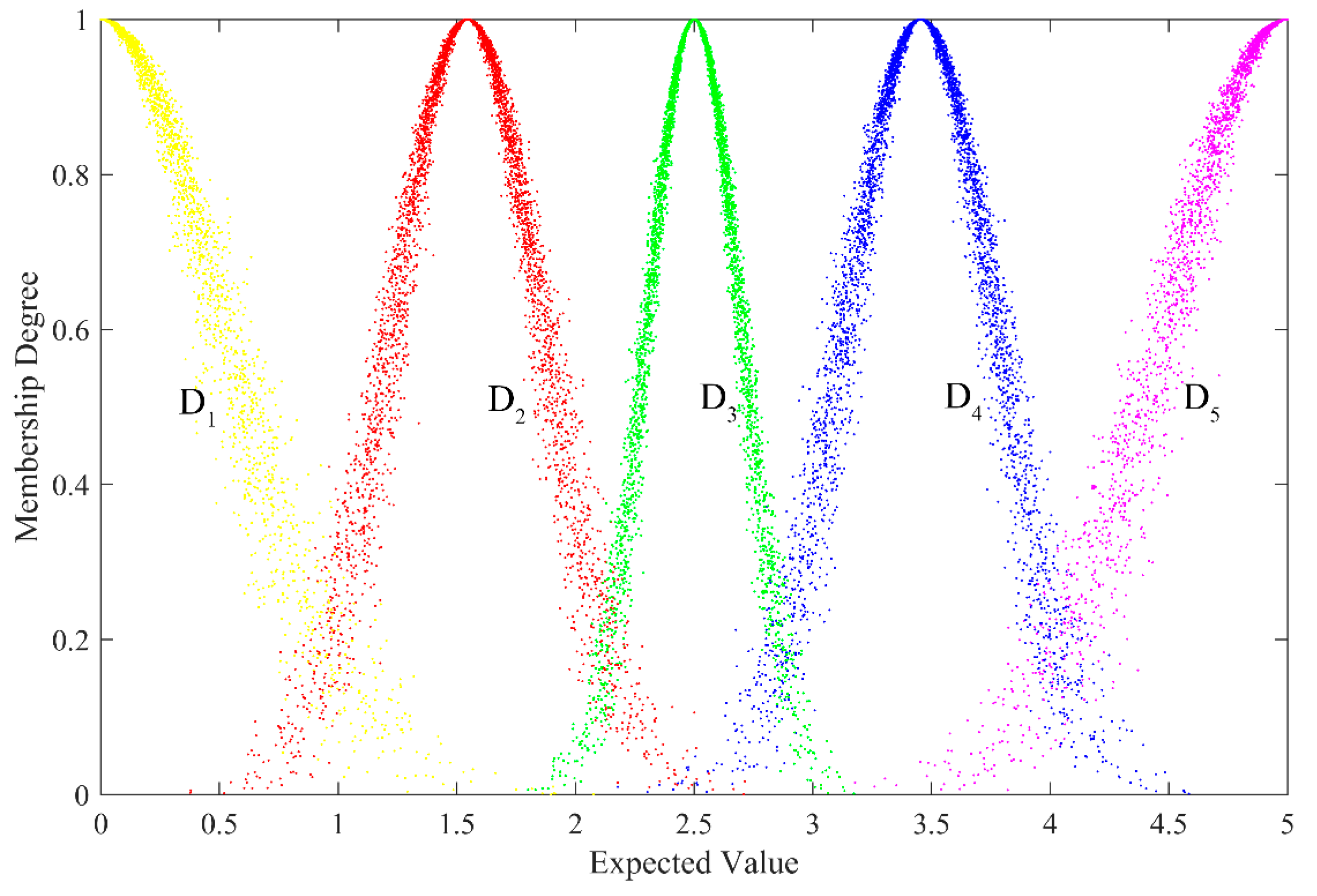
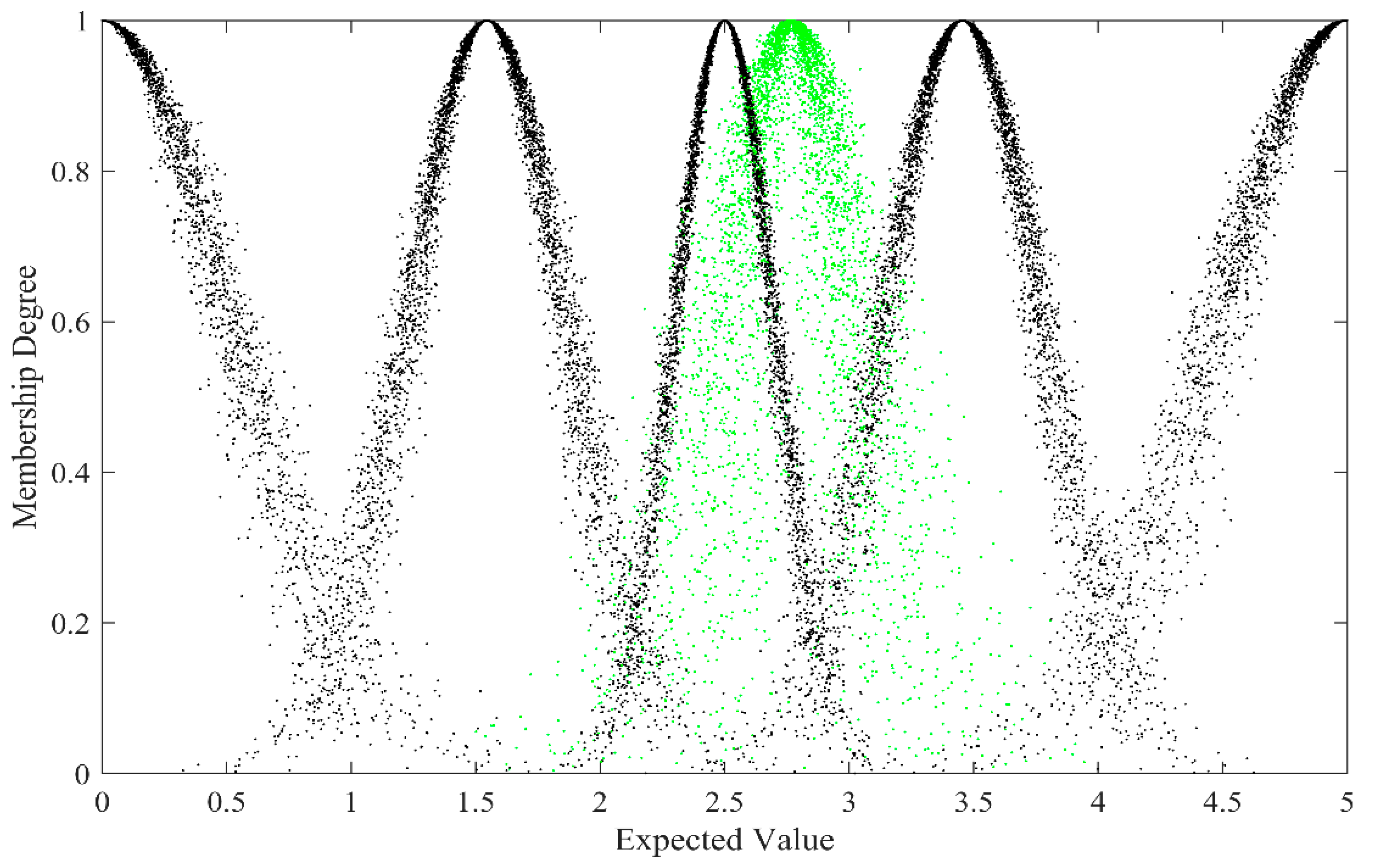
The golden section cloud generation method is used to calculate and determine the assignment clouds of different WRCC levels based on the aforementioned classifications. Within the domain of [0,5], the boundary values of 0 and 5 are taken as the cloud’s expected value of level D1 and D5, respectively. The intermediate value of 2.5 was taken as the cloud’s expected value of level D3. The cloud’s expected values of level D2 and D4 follow the golden section method. For the values of adjacent expectation, entropy and hyper entropy (Ex, En, He), the smaller value was 0.618 times the larger value. The determination of the entropy value follows the ‘3 En rule’ and the hyper entropy value was about 0.1 times the entropy value. According to these rules and methods, the eigenvalues of the assignment clouds of different WRCC levels were calculated (Table 3), and the corresponding assignment clouds are shown in Figure 2.
(3)
The WRCCA index clouds calculated by cloud operations
Based on the comprehensive evaluation sets and the assignment clouds at different WRCC levels of each subsystem, the evaluation index cloud of each subsystem ξ i is calculated by using the weighted average principle and the cloud algebraic operation rules, which is expressed as Equation (36):
ξ i = j = 1 n b i j c j j = 1 n b i j
where ξ i (i = 1, 2, …, m) is the evaluation index cloud of each subsystem, i is the number of subsystems, b i j (j = 1, 2, …, n) is the element in i-th row and j-th column of the comprehensive evaluation set for each subsystem, j is the number of evaluation levels and c j is the assignment cloud at a certain evaluation level for each subsystem. Finally, the evaluation index cloud of WRCC ξ is calculated based on the weight cloud and evaluation index cloud of each subsystem, that is,
ξ = i = 1 m ξ i w i
where ξ i and w i are the evaluation index cloud and weight cloud of each subsystem, respectively.

3. Application

3.1. Study Area

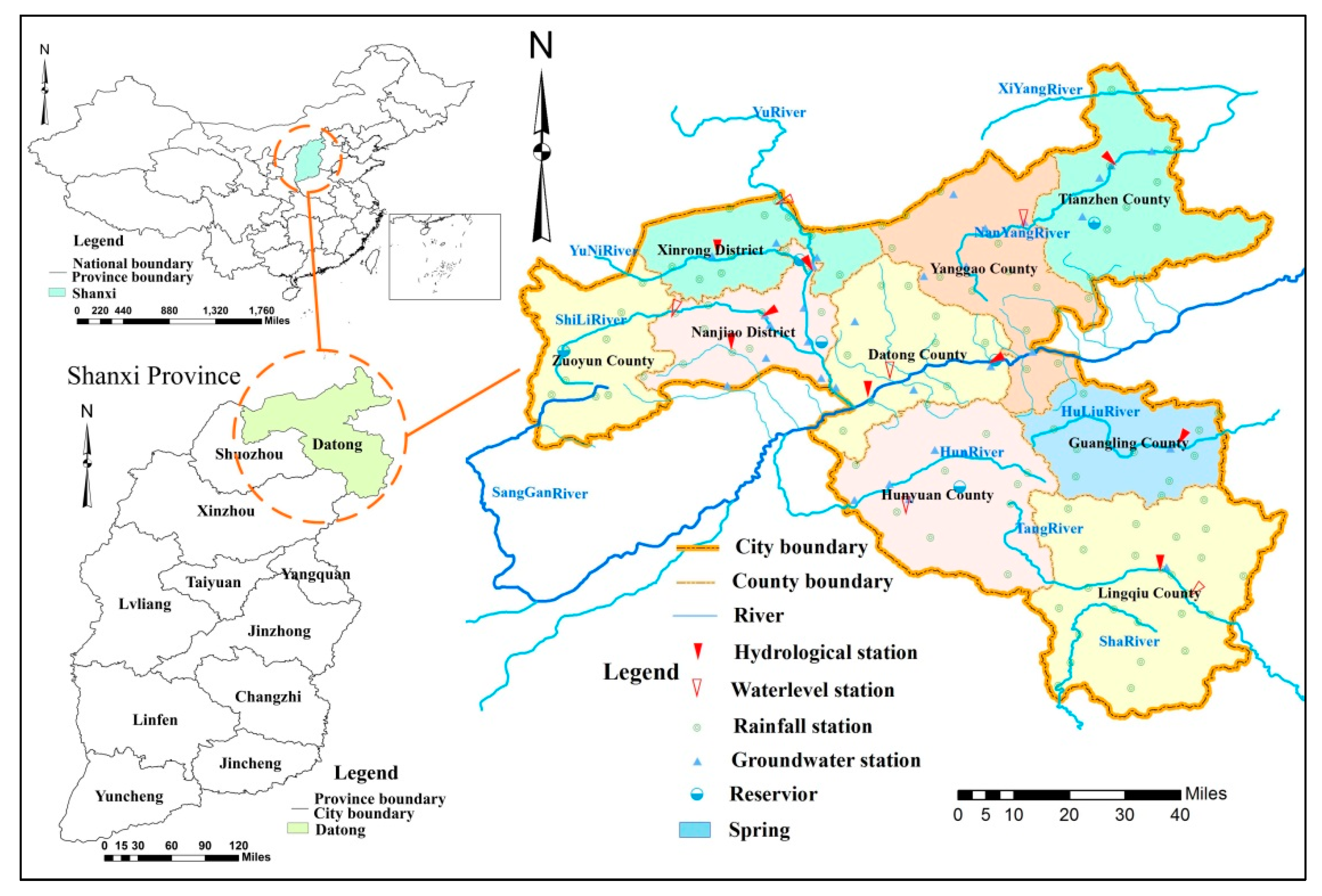
As a case study, we apply and validate the proposed FCE-AHP-CM hybrid approach for WRCCA in Datong City, which is located at the north of Shanxi Province in China (Figure 3). It has a continental monsoon climate with the average temperature of 6–8 °C, average annual rainfall of 421.4 mm, and average evaporation of 1067.4 mm. Dating City is a typical arid and semiarid region in North China, whose rainfalls are very unevenly distributed in spaces with great changes within and between years. As shown in Figure 3, the main rivers include Sanggan River, Yuhe River, Shili River, Yuni River, Hun River, Nanyang River, Xiyang River, Huliu River, and Tang River, which belong to the Yongding River and Daqing River systems of the Haihe River Basin. There are six large and medium-sized reservoirs, nine hydrological stations, six water level stations, eight spring stations, 193 rainfall stations, 298 groundwater observation stations, and 30 water quality monitoring sections.
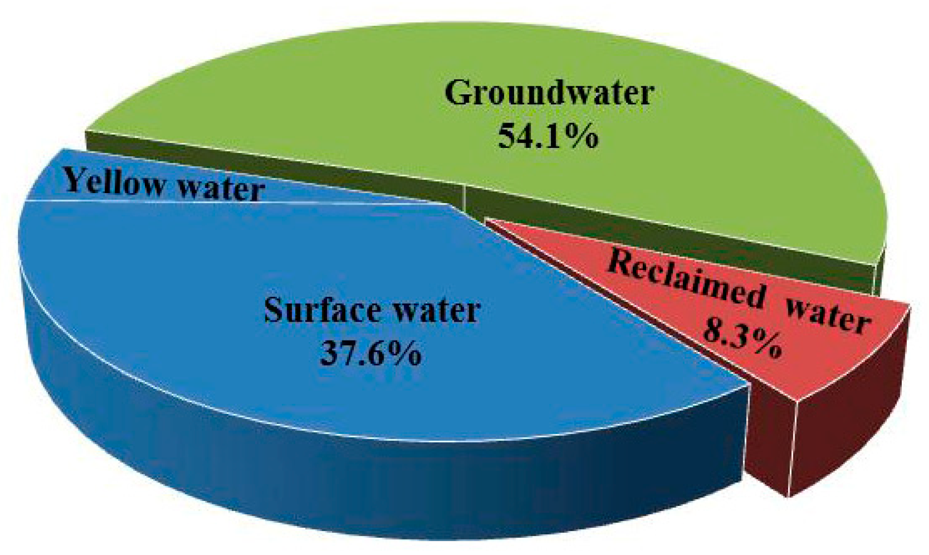
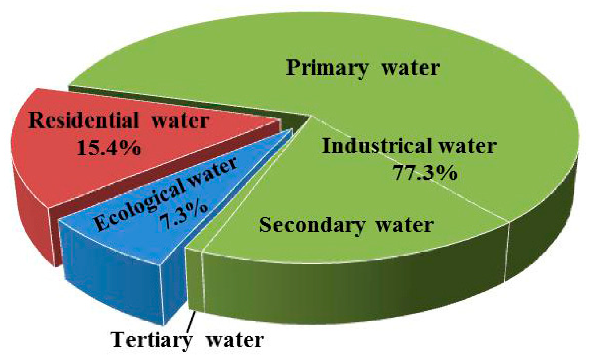
The water resources in Datong City are severely shorted and in a high level of development and utilization. In 2017, the average amount of water resources per capita in Datong City was only 277 m3 and the rate of surface water resource exploitation was 44.9%. The groundwater extraction coefficient was 0.95. The total amount of local water resources is 954.32 million m3, of which the amount of natural runoff is 479.02 million m3, the volume of groundwater resources is 732.49 million m3, and the repeat volume is 257.19 million m3. The total amount of water consumption is 615.11 million m3, which include 231.16 million m3 of surface water, 332.79 million m3 of groundwater consumption and 51.16 million m3 of reclaimed water (Figure 4). The water can be classified by water usage, which include 94.86 million m3 for residential use, 475.56 million m3 for industrial use, and 44.69 million m3 for ecological use (Figure 5).

3.2. Evaluation Indicator System Construction and Data Preparation for WRCCA in the Study Area

The text matching method was used for document matching and indicator query in the study area. After counting the occurrence frequency of each indicator in the query results, a total of 36 indicators with the frequency of the top 30% were selected. By collecting statistical data and water consumption data of various industries from the Datong Statistical Yearbook, the Datong Water Resources Bulletin, the Measured and Historical Compilation Data of Hydrology and Water Resources Survey Station of Shanxi Province, the Spearman rank correlation analysis method was used to calculate the correlation of indicators with Equation (2). Since the correlation coefficients between precipitation and precipitation in the flood season, annual runoff and annual runoff depth are 0.92 and 0.95, respectively, two indicators were removed. Using the gray correlation method to further select the indicators with Equations (3)–(8), we found that the correlations of seven indicators, such as downrange of groundwater depth, water consumption of ten-thousand CNY (USD 1426) industrial output value, vegetation coverage, industrial wastewater discharge, domestic sewage discharge, mine drainage, and industrial output value as a percentage of GDP, were relatively weak. After screening them, the evaluation indicator system for WRCCA in the study area, consisting of 27 indicators in four subsystems, was finally constructed (Table 4).
The maximum and minimum values of every indicator in Datong City over 30 years were evenly divided into five levels. If there were few other close values distributed near the individual maximum and minimum values, they were traded off. From Equations (9)–(11), each indicator level range was obtained, and after further adjustment in accordance with national or industry standards, the evaluation indicator level standards were finally determined (Table 5), and as examples, only the corresponding data of every indicators of the study area in 2017 are shown in Table 5.

3.3. Results of WRCCA in the Study Area

3.3.1. Calculation of the Weights Clouds for Subsystems and Indicators

In this case study, we selected three experts in the field of WRCCA from the Experts Database, and after consulting with them, the opinions of each expert on relative importance’s of subsystems and indicators were respectively obtained. Then using the floating cloud model, we aggregated the judgement matrices of subsystems and indicators given by different experts (Table 6, Table 7, Table 8, Table 9 and Table 10).
By using Equations (27)–(29) and the data of the study area in 2017, the weights clouds eigenvalues of each subsystem and indicator were calculated (Table 11). The results showed that the hydrology subsystem has the largest weights and the most significant effects on the WRCC, followed by the water resource utilization and the water ecological environment subsystems, and the economic and social subsystem has the smallest weights and negative effects on the WRCC. The top 10 indicators are: precipitation in flood season, surface water quality index, runoff depth, ecological environment water use rate, GDP per capita, population density, water resources per capita, groundwater extraction coefficient, development and utilization of surface water resources, and dilution ratio.

3.3.2. Calculation of the Membership Matrices and Comprehensive Evaluation Sets of Subsystems

By using Equation (12), the membership matrices of evaluation indicators of each subsystem of the study area in 2017 were calculated as follows.
R Hydrology = [ 0.091 0.678 0.336 0.001 0.001 0.129 0.866 0.191 0.000 0.001 0.162 0.961 0.118 0.000 0.000 0.027 0.145 0.924 0.027 0.010 0.001 0.000 0.150 0.925 0.145 0.000 0.000 0.064 1.000 0.208 ]
R Water   resources   utilization = [ 0.014 0.052 0.992 0.082 0.020 0.099 0.733 0.290 0.001 0.002 0.154 0.936 0.133 0.001 0.001 0.000 0.000 0.000 0.018 0.947 0.002 0.000 0.069 0.999 0.190 0.141 0.926 0.146 0.000 0.001 0.000 0.000 0.000 0.000 0.964 0.000 0.000 0.003 0.365 0.566 0.143 0.905 0.163 0.000 0.002 0.000 0.000 0.000 0.027 0.920 0.000 0.000 0.001 0.295 0.612 ]
R Water   ecological   environment = [ 0.000 0.000 0.000 0.000 0.655 0.000 0.000 0.000 0.006 0.989 0.000 0.000 0.000 0.003 1.000 0.004 0.007 0.726 0.304 0.038 0.001 0.001 0.213 0.826 0.122 ]
R Economy   and   society = [ 0.016 0.075 0.996 0.063 0.012 0.046 0.357 0.659 0.005 0.004 0.000 0.000 0.000 0.012 0.960 0.000 0.000 0.000 0.062 0.826 0.123 0.840 0.211 0.000 0.001 ]
Then, by using Equation (13), the comprehensive evaluation set of all the subsystems of the study area in 2017 was calculated after the dot multiplication operation between the evaluation indicators weights clouds and membership matrices of each subsystem:
B = [ ( 0.091 , 0.051 , 0.051 ) ( 0.611 , 0.349 , 0.348 ) ( 0.277 , 0.146 , 0.146 ) ( 0.165 , 0.125 , 0.124 ) ( 0.030 , 0.021 , 0.021 ) ( 0.059 , 0.033 , 0.034 ) ( 0.374 , 0.209 , 0.215 ) ( 0.203 , 0.132 , 0.135 ) ( 0.080 , 0.046 , 0.047 ) ( 0.380 , 0.203 , 0.197 ) ( 0.001 , 0.001 , 0.001 ) ( 0.002 , 0.001 , 0.001 ) ( 0.194 , 0.135 , 0.140 ) ( 0.345 , 0.286 , 0.292 ) ( 0.432 , 0.248 , 0.240 ) ( 0.039 , 0.024 , 0.025 ) ( 0.268 , 0.173 , 0.175 ) ( 0.524 , 0.359 , 0.356 ) ( 0.027 , 0.020 , 0.019 ) ( 0.225 , 0.167 , 0.165 ) ]

3.3.3. Calculation of the Evaluation Index Clouds for WRCCA in the Study Area

The WRCC evaluation index clouds of each subsystem of the study area in 2017 were calculated by using Equation (36) based on the comprehensive evaluation set and different levels of the assignment clouds. En and He were normalized by analyzing the entropy ‘En’ and hyper entropy ‘He’, as well as through comparing them with the eigenvalues of the assignment clouds. Finally, by using Equation (37), the WRCC evaluation index clouds were calculated. Their results are shown in Table 12.

3.3.4. Determination of the Evaluation Levels for WRCCA in the Study Area

According to their eigenvalues in Table 12, the corresponding evaluation index clouds of WRCC and each subsystem of Datong City in 2017 are shown in Figure 6 and Figure 7, respectively. From Figure 6, it can be seen intuitively that the WRCC evaluation index cloud of Datong City in 2017 is located between the clouds of D3 and D4 levels, and is closer to the D3 level cloud. It can be inferred that the WRCC level of Datong in 2017 is D3, which is in a non-overloaded state. From comparison between the evaluation index cloud and the level assignment cloud, it can be seen that the distribution of the evaluation index cloud is relatively concentrated, and the values of both entropy ‘En’ and hyper entropy ‘He’ are reasonable. The expected value Ex takes a lead in determining the level of WRCC. It is credible to obtain the level of WRCC from Ex.
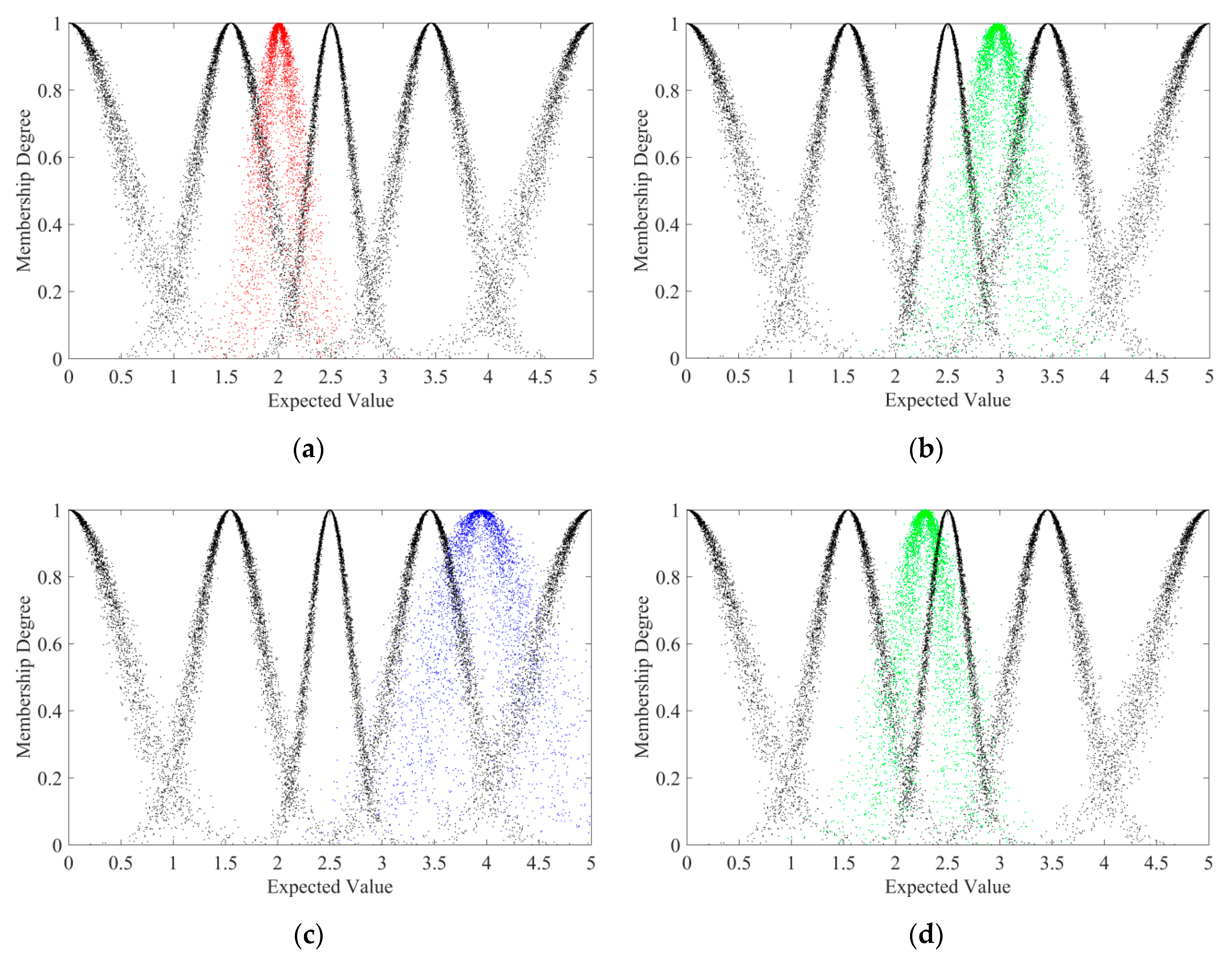
It is known, from Figure 7, that the WRCC evaluation index cloud of the hydrology subsystem of the study area in 2017 is located between the D2 and D3 level clouds, which is closer to the D2 level cloud, and tends to approach the D3 level cloud. This means that the WRCC level of hydrology subsystem is D2, which is in an overload state and has a tendency to develop towards a non-overloaded state. The WRCC evaluation index cloud of the water resources utilization subsystem is located between the D3 and D4 level clouds, which is closer to the D3 level cloud, and tends to approach the D4 level cloud. It means that the WRCC level of water resources utilization subsystem is D3, which is in a non-overloaded state and has a tendency to develop towards a good carrying state. The WRCC evaluation index cloud of the water ecological environment subsystem is located between the D4 and D5 level clouds, which is closer to the D4 level cloud. This means that the WRCC level of water ecological environment subsystem is D4, which is in a good carrying state. The WRCC evaluation index cloud of the economy and society subsystem is located between the D2 and D3 level clouds, which is closer to the D3 level cloud. This means that the WRCC level of economy and society subsystem is D3, which is in a non-overloaded state.

3.4. Validation and Analysis of WRCCA in the Study Area

3.4.1. WRCCA Results Validation in the Study Area

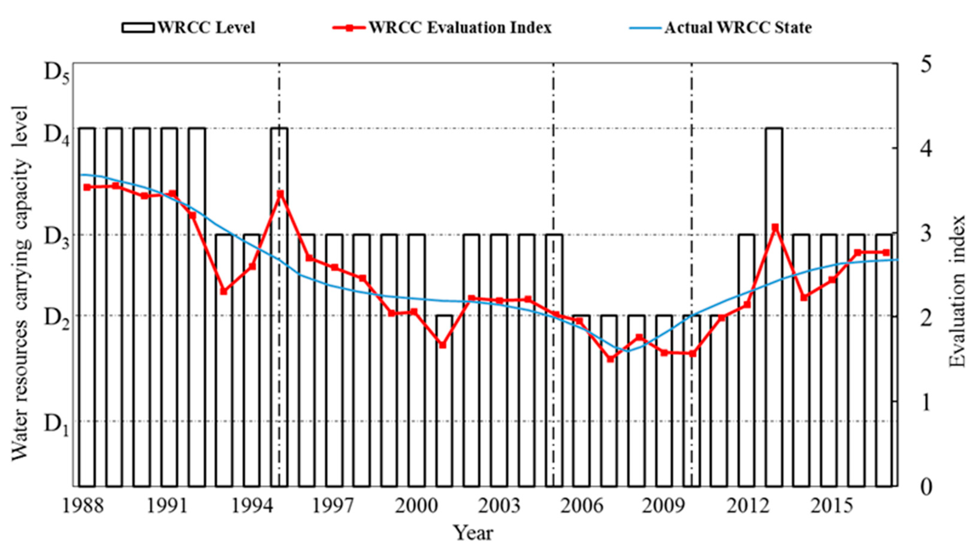
Similar to the above WRCCA calculations of the study area in 2017, the WRCC levels (the histogram in Figure 8) and evaluation indexes (the red line in Figure 8) of Datong City from 1988 to 2016 were also obtained. It is shown that the WRCC of Datong City gradually decreased from D4 level to D2 level and then restored to D3 level from 1988 to 2017. That is, the WRCC level experienced a transition from being good carrying to overloaded carrying, and finally restored to be non-overloaded carrying. The WRCC levels were D4 from 1988 to 1992, and then gradually weakened. In most cases, the levels were D3 from 1993 to 2005. There were two exceptions in 1995 with the level of D4 and in 2001 with the level of D2. The levels of WRCC were D2 from 2006 to 2011, which was an overloaded state. The WRCC levels were mostly D3 in 2012–2017 with an exception of D4 in 2013, which restored to a non-overloaded state.
According to the annual ‘Datong City Government Work Report’, ‘Datong City Water Resources Evaluation and Allocation Schemes’, ‘Datong City Water Resources Globalization Allocation Schemes’, and the actual development analysis of Datong City, the annual actual WRCC states from 1988 to 2017 have been collected (the blue line in Figure 8). It can be seen that the natural hydrological conditions of the study area were relatively good and the water resources utilization potential was large in the late 1980s and early 1990s. During this period, the economy and society were not well developed and the water demands were low. Thus, the WRCC was relatively strong, generally in a good carrying state, and showed a gradual weakening trend. From the mid-1990s to the end of the ‘10th Five-Year Plan’ period (2001–2005), the WRCC was basically in a non-overloaded state and showed a steady downward trend. During the ‘11th Five-Year Plan’ period (2006–2010), the water demands and the amount of waste water discharges increased rapidly with the accelerated urbanization process and the development of economy and society. As a result, the quality of the water environment deteriorated, the WRCC was in an overloaded state and showed a trend of decreasing first and then increasing. With the implementation of the ‘12th Five-Year Plan’ (2011–2015), a large number of water conservancy projects and water-saving projects started to be constructed. During this period, ‘three red lines’ were established, ‘the most stringent water resources management system’ was implemented, and the water-saving awareness of the whole society was raised. The WRCC therefore has been effectively improved, and returned to a non-overloaded state and showed a gradual upward trend. In 1993, 2001, and 2013, due to sudden changes in hydrological conditions such as precipitation, the WRCC has changed significantly. Excluding the above 3 special years, the WRCC of Datong City has experienced the changes from a good carrying state to a non-overloaded state, then to an overloaded status, and finally restored to a non-overloaded state.
From comparisons between the WRCCA results calculated with the FCE-AHP-CM hybrid approach and the corresponding actual WRCC states of the study area from 1988 to 2017 in Figure 8, it could be found that not only the differences of WRCC levels in most years are very small, but also their change tendencies in the past 30 years are very similar. In addition, by comparing the results of this study with previous studies, it was found that the conclusions obtained are similar. Regarding the WRCCA results in Datong City, this paper and those by Wang et al. [40] and Liu [41] have shown that the water resources carrying states in 2000 and 2010 calculated by different evaluation methods were consistent and the variation trend of the WRCC assessed by different evaluation models was similar. At the same time, the novel hybrid FCE-AHP-CM approach proposed in this paper has the special superiority in comprehensively dealing with the fuzziness and randomness, and therefore not only could accurately assess the WRCC, but also could significantly increase the robustness and intuition of WRCCA results. In the assessment of the WRCC, this paper and those by Xi et al., Wen et al., Zhang, Peng et al., Wu et al., Yu et al., and Zhang [42,43,44,45,46,47,48] found that the WRCC has been effectively improved and showed an increasing trend after the ‘11th Five-Year Plan’ in China. The hydrological conditions such as precipitation have a great influence on the WRCC. The aforementioned comparative discussion further verifies the accuracy, reliability, and stability of the novel FCE-AHP-CM hybrid approach for WRCCA proposed in this paper.

3.4.2. Mechanism Analyses of the WRCC Changes in the Study Area Based on the Evaluation Index

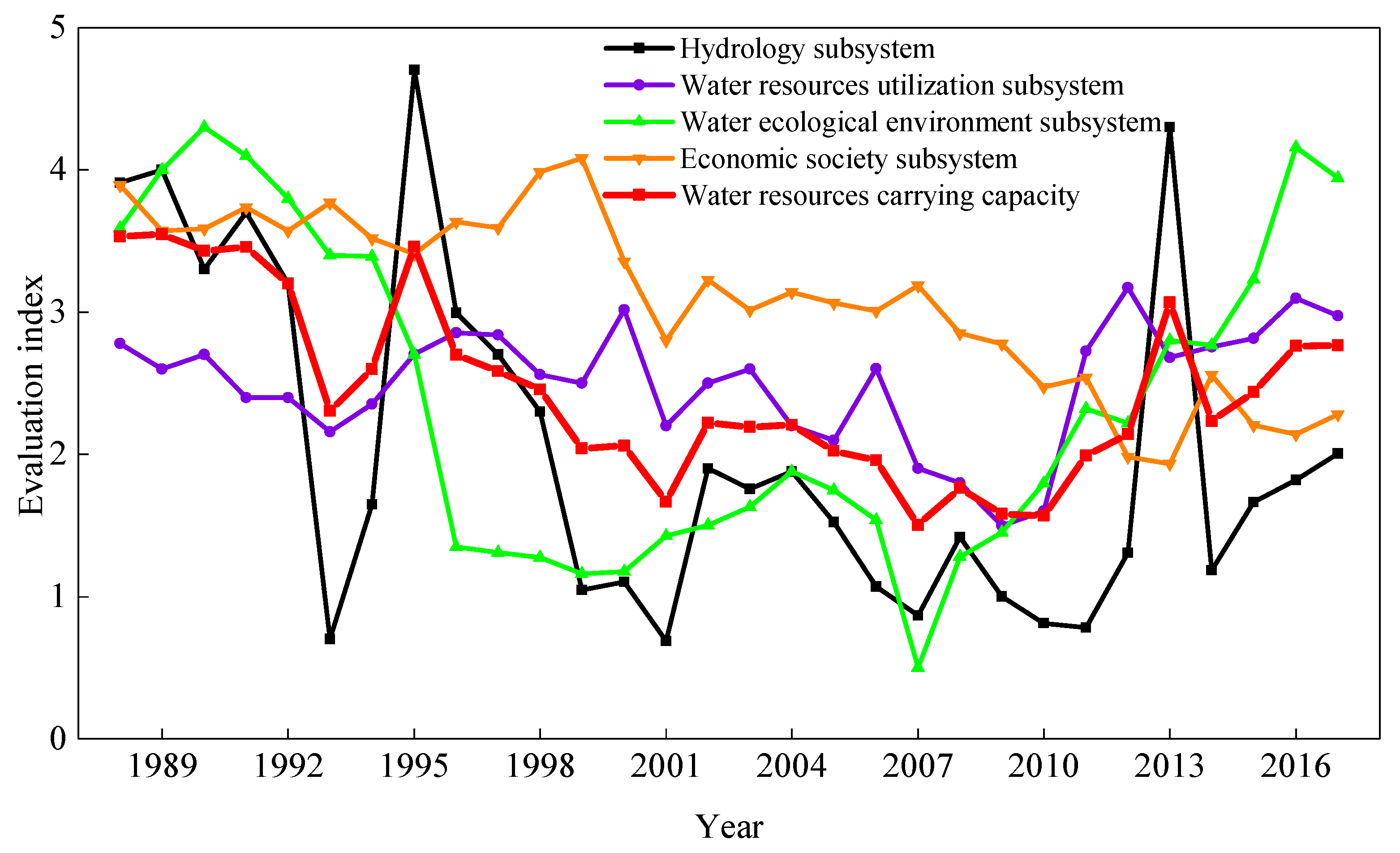
In order to analyze the possible mechanisms of the WRCC changes in the study area from 1988 to 2017, we could compare the comprehensive evaluation indexes of WRCC and the corresponding evaluation indexes of every subsystems (Figure 9). As known in the above subsection, the evaluation indexes of WRCC showed an overall downward trend, generally obvious between 1988 and 2001 except for sudden changes in individual years. The downward trend became flattened from 2002 to 2011 and began to gradually increase since 2012. The highest and lowest values of the comprehensive evaluation indexes were 3.548 in 1989 and 1.503 in 2007, respectively. Moreover, the peak values were found in 1995 and 2013, and the valley values were found in 1993 and 2001 (the red line in Figure 9).
The evaluation indexes of the hydrology subsystem showed a declining trend (the black line in Figure 9). The decline rate was large from 1988 to 2001, became smaller during 2002 to 2010, and then began to increase from 2011. The two highest values were 4.704 in 1995 and 4.301 in 2013, and the two lowest values were 0.701 in 1993 and 0.687 in 2001. These changes were highly consistent with the WRCC evaluation index changes, which indicated that the WRCC in the study area was greatly affected by the hydrological conditions.
Shown as the blue line in Figure 9, the evaluation indexes of the water resources utilization subsystem varied slightly from 1988 to 2017. A slow downward trend was observed from 1988 to 2010, followed by a sudden increase in 2011 and then steadily rose thereafter. The two highest values were 3.175 in 2012 and 3.098 in 2016, and the lowest value was 1.501 in 2009. The evaluation indexes changes of the water ecological environment subsystem could be divided into two stages (the green line in Figure 9). The indexes decreased rapidly from 1988 to 2007, and started to increase from 2008 with an obvious upward trend. The two highest index values were 4.301 in 1990 and 4.159 in 2016. The lowest index value was 0.501 in 2000. It could be seen that the tendency of WRCC evaluation indexes changes were basically consistent with the evaluation indexes changes tendency of the water resources utilization subsystem and water ecological environment subsystem, which indicated that the WRCC in the study area was affected by these two subsystems.
According to the orange line in Figure 9, the evaluation indexes of the economic and social subsystem generally showed a downward trend. It fluctuated from 1988 to 1997, slightly rose between 1998 and 1999, rapidly decreased in the next 2 years, fell gently in 2002, reached the lowest value in 2013, and then started to rebound slightly from 2014. The two highest index values were 3.987 in 1998 and 4.081 in 1999. The two lowest index values were 1.982 in 2012 and 1.936 in 2013. It could be found that the evaluation indexes changes of the WRCC and the economic and social subsystem showed opposite tendencies. The faster the development was, the lower the index would be.

4. Conclusions

It has been well known that the WRCC in a region is affected and decided by many factors. However, the viewpoints of different experts on their influences could not always be the same. There are strong uncertainties such as fuzziness and randomness in the process of WRCCA. In order to solve these problems, we proposed a novel hybrid approach by integrating the FCE and AHP methods with the cloud model. The main conclusions of this paper are as follows.
The evaluation indicator system is the key fundamental of WRCCA. Four evaluation subsystems, including hydrology, water resources utilization, water ecological environment, and economy and society, were constructed based on the evaluation rules with the former two subsystems as constraints, and the latter two subsystems as optimization goals. For the selection and screening of the indicators in each subsystem, the qualitative and quantitative methods such as text matching, Spearman rank correlation analysis and gray correlation are very effective, especially in the big data area.
The FCE method could solve the fuzziness problem in WRCCA, and the AHP method could be helpful to calculate the weights of multilayer indicators for the FCE method. In addition, the cloud model could be used to improve the FCE and AHP methods. For the integrations of AHP with CM, the relative importance’s of indicators could be scaled with the expectation, entropy and hyper entropy of the cloud model, the aggregation of judgement matrices could be described by the floating cloud model, and finally the weights clouds of subsystems and indicators in WRCCA could be obtained, which would greatly reduce the randomness in the weights calculations caused by different experts’ subjective opinions. For the integrations of FCE with CM, the different levels of comment sets could be expressed with the eigenvalues of cloud models, the membership degree matrix could be calculated by the forward cloud generator, the assignment clouds of WRCC levels could be determined by golden section cloud generation, and finally, the WRCCA index clouds could be obtained by cloud operations, which would effectively blur the fuzziness of the WRCC level boundaries and give more intuitive evaluation results. As a case study, the FCE-AHP-CM hybrid approach for WRCCA proposed in this paper was applied to Datong City of Shanxi Province in North China, it was shown that the WRCC in the study area could be accurately assessed with the hybrid approach, and especially, since the novel hybrid approach has the particular advantages to comprehensively deal with the fuzziness and randomness in WRCCA, the robustness and intuition of results could be significantly enhanced. By the way, by comparing the comprehensive evaluation index cloud of WRCC and the evaluation index cloud of each subsystem, the possible corelationships between the WRCC and impact factors could be analyzed and revealed.

Author Contributions

B.R. and Q.Z. conceived and designed the research theme. B.R. and F.Y. collected the data and designed the methods. J.R. and S.Y. analyzed the data and interpreted the results. B.R. and Q.Z. wrote and edited the manuscript. All authors have read and agreed to the published version of the manuscript.

Funding

This research was partially supported by the National Natural Science Foundation of China (Grant no. 41672263).

Acknowledgments

The authors thank the anonymous reviewers and academic editors of the journal for their useful comments and suggestions to improve the manuscript.

Conflicts of Interest

The authors declare no conflict of interest.

References

  1. Rijsberman, M.A.; Ven, F.H.M.V.D. Different approaches to assessment of design and management of sustainable urban water systems. Environ. Impact Assess. Rev. 2000, 20, 333–345. [Google Scholar] [CrossRef]
  2. Park, R.; Assimilation, B.E. Introduction to the Science of Sociology; University of Chicago Press: Chicago, IL, USA, 1921. [Google Scholar]
  3. UNESCO; FAO. Carrying Capacity Assessment with a Pilot Study of Kenya: A Resource Accounting Methodology for Sustainable Development; United Nations Educational, Scientific and Cultural Organization: Paris, France, 1985. [Google Scholar]
  4. National Research Council. Areview of the Florida Keys Carring Capacity Study; National Academy Press: Washington, DC, USA, 2002. [Google Scholar]
  5. Xinjiang Water Resources Soft Science Research Group. Strategies and countermeasures for the development of Xinjiang water resources and its carrying capacity. Water Res. Hydropower Eng. 1989, 6, 2–9. (In Chinese) [Google Scholar]
  6. Shi, Y.F.; Qu, Y.G. The Carrying Capacity of Water Resources and Its Reasonable Use of Urumqi River; Science Press: Beijing, China, 1992. (In Chinese) [Google Scholar]
  7. Xu, Y.P. A study of comprehensive evaluation of the water resource carrying capacity in the arid area—A case study in the Hetian river basin of Xinjiang. J. Nat. Res. 1993, 3, 229–237. (In Chinese) [Google Scholar]
  8. Feng, S.Y.; Liu, G.Q. A Holistic Framework for Sustaining Water Resources Utilization. Adv. Water Sci. 1997, 4, 2–8. (In Chinese) [Google Scholar]
  9. Hui, Y.H.; Jiang, X.H.; Huang, Q.; Xue, X.J. On system dynamic simulation model of water resources bearing capacity in duality mode. Geogr. Res. 2001, 2, 191–198. (In Chinese) [Google Scholar]
  10. Xia, J.; Zhu, Y.Z. The measurement of water resources security: A study and challenge on water resources carrying capacity. J. Nat. Res. 2002, 3, 262–269. (In Chinese) [Google Scholar]
  11. He, R.W.; Liu, S.Q.; Liu, Y.W. Application of system dynamics in analyzing the carrying capacity of water resources in karst region of Southwest china—A case study in Bijie region, Guizhou province. Sci. Geogr. Sin. 2011, 31, 1376–1382. [Google Scholar]
  12. Liu, H.Q. A study on the change trends of regional water resource carrying capacity. Lect. Notes Electr. Eng. 2012, 113, 1375–1380. [Google Scholar]
  13. Meng, L.H.; Chen, Y.N.; Li, W.H.; Zhao, R.F. Fuzzy comprehensive evaluation model for water resources carrying capacity in Tarim river basin, Xinjiang, China. Chin. Geogr. Sci. 2009, 19, 89–95. [Google Scholar] [CrossRef]
  14. Gong, L.; Jin, C.L. Fuzzy Comprehensive Evaluation for Carrying Capacity of Regional Water Resources. Water Res. Manag. 2009, 23, 2505–2513. [Google Scholar] [CrossRef]
  15. Gao, Y.; Zhang, S.; Xu, G.W.; Su, H.M.; Zhang, Y. Study on water resources carrying capacity in Hefei city. Adv. Mat. Res. 2012, 610–613, 2701–2704. [Google Scholar] [CrossRef]
  16. Liu, J.J.; Dong, S.C.; Li, Z.H. Comprehensive evaluation of china’s water resources carrying capacity. J. Nat. Res. 2011, 26, 258–269. (In Chinese) [Google Scholar]
  17. Guo, Q.; Wang, J.Y.; Zhang, B. Comprehensive evaluation of the water resources carrying capacity based on DPSIMR. J. Nat. Res. 2017, 32, 484–493. (In Chinese) [Google Scholar]
  18. Chen, Y.B.; Chen, J.H.; Li, C.X.; Feng, Z.Y. Indicators for water resources carrying capacity assessment based on driving forces-pressure-state-impact-response model. J. Hydraul. Eng. 2004, 7, 98–103. (In Chinese) [Google Scholar]
  19. Jin, J.L.; Shen, S.X.; Chen, M.L.; Li, J.Q.; Guo, X.N.; Chang, T. Application of genetic analytic hierarchy process in screening the evaluation index system of regional water resources carrying capacity. J. North China Univ. Water Res. Elec. Power (Nat. Sci.) 2019, 40, 1–6. (In Chinese) [Google Scholar]
  20. Wang, J.H.; Zhai, Z.L.; Sang, X.F.; Li, H.H. Study on index system and judgment criterion of water resources carrying capacity. J. Hydraul. Eng. 2017, 48, 1023–1029. [Google Scholar]
  21. Yang, Z.Y.; Song, J.X.; Cheng, D.D.; Xia, J.; Li, Q.; Ahamad, M.I. Comprehensive evaluation and scenario simulation for the water resources carrying capacity in Xi’an city, China. J. Environ. Manag. 2019, 230, 221–233. [Google Scholar] [CrossRef]
  22. Chi, M.B.; Zhang, D.S.; Fan, G.W.; Zhang, W.; Liu, H. Prediction of water resource carrying capacity by the analytic hierarchy process-fuzzy discrimination method in a mining area. Ecol. Indic. 2019, 96, 647–655. [Google Scholar] [CrossRef]
  23. Dai, D.; Sun, M.D.; Xu, X.Q.; Lei, K. Assessment of the water resource carrying capacity based on the ecological footprint: A case study in Zhangjiakou city, north china. Environ. Sci. Pollut. Res. 2019, 26, 11000–11011. [Google Scholar] [CrossRef]
  24. Wu, L.; Su, X.L.; Ma, X.Y.; Kang, Y.; Jiang, Y.N. Integrated modeling framework for evaluating and predicting the water resources carrying capacity in a continental river basin of northwest china. J. Clean. Prod. 2018, 204, 366–379. [Google Scholar] [CrossRef]
  25. Ma, L.; Zhao, J.H.; Hong, M.; Chen, L.L. Application of set pair analysis model based on entropy weight for comprehensive evaluation of water resources carrying capacity. Appl. Mech. Mater. 2012, 195–196, 764–769. [Google Scholar] [CrossRef]
  26. Zadeh, L.A. Fuzzy Sets. Inf. Control 1965, 8, 338–353. [Google Scholar] [CrossRef] [Green Version]
  27. Saatyt, L. The Analytical Hierarchical Process; McGraw-Hill: New York, NY, USA, 1980. [Google Scholar]
  28. Rodriguez, R.; Lev, B. Models, methods, concepts and applications of the analytic hierarchy process. Interfaces 2002, 32, 93. [Google Scholar]
  29. Saaty, T.L. The Analytic Hierarchy Process: Decision Making in Complex Environments; Springer: Boston, MA, USA, 1984. [Google Scholar]
  30. Vaidya, O.S.; Kumar, S. Analytic hierarchy process: An overview of applications. Eur. J. Oper. Res. 2006, 169, 1–29. [Google Scholar] [CrossRef]
  31. Kazakidis, V.N.; Mayer, Z.; Scoble, M.J. Decision making using the analytic hierarchy process in mining engineering. Min. Technol. 2004, 113, 30–42. [Google Scholar] [CrossRef]
  32. Kumar, R.; Anbalagan, R. Landslide susceptibility mapping using analytical hierarchy process (AHP) in Tehri reservoir rim region, Uttarakhand. J. Geol. Soc. India 2016, 87, 271–286. [Google Scholar] [CrossRef]
  33. Saaty, T.L. Erratum: “A scaling method for priorities in hierarchical structures”. Mathematical 1979, 3, 234–281. [Google Scholar]
  34. Li, D.Y.; Meng, H.J.; Shi, X.M. Membership clouds and membership cloud generators. Comput. Res. Dev. 1995, 6, 15–20. (In Chinese) [Google Scholar]
  35. Wang, S.G. Cloud model for service selection. In Proceedings of the 2011 IEEE Conference on Computer Communications Workshops, Shanghai, China, 10–15 April 2011; IEEE: Shanghai, China, 2011. [Google Scholar]
  36. Liang, M.; Xun, Y.; Yi, Z.X.; Fu, X.H. The qualitative forecasting model based on the cloud model and its application in macrosiphum avenae. Sci. Agric. Sin. 2002, 35, 654–659. [Google Scholar]
  37. Liu, D.D.; Chen, X.H.; Lou, Z.H. Analysis on characteristics of spatial-temporal precipitation distribution based on cloud model. J. Hydraul. Eng. 2009, 40, 850–857. [Google Scholar]
  38. Yang, S.M.; Han, X.Q.; Cao, B.; Li, B.; Yan, F. Cloud-model-based method for risk assessment of mountain torrent disasters. Water 2018, 10, 830. [Google Scholar] [CrossRef] [Green Version]
  39. Li, J.; Zhang, Q.W.; Yan, F.; Zhong, M. A cloud model-based multi-level fuzzy comprehensive evaluation approach for financing credit of scientific & technological small-medium enterprises. J. Differ. Equ. Appl. 2016, 23, 1–14. [Google Scholar]
  40. Wang, Z.J.; Liao, S.H.; Wu, X.F.; Zhao, J.S.; Gan, H. Water resources carrying capacity in Datong City. South North Water Transf. Water Sci. Technol. 2007, 5, 47–50. (In Chinese) [Google Scholar]
  41. Liu, D. Research on Regional Water Resources Carrying Capacity Assessment—A Case Study of Datong City. Master’s Thesis, North China Electric Power University, Baoding, China, March 2015. (In Chinese). [Google Scholar]
  42. Xi, D.C.; Xu, X.Y.; Han, D.M.; Yang, Z.W. Evaluating water resources carrying capacity in Beijing-Tianjin-Hebei region. J. Beijing Norm. Univ. (Nat. Sci.) 2017, 53, 575–581. (In Chinese) [Google Scholar]
  43. Wen, L.H.; Liu, H.Y.; Yao, H.J.; Zhang, G.L. Study on water resources carrying capacity in eight provinces of northern China. Res. Soil Water Conserv. 2013, 20, 168–176. (In Chinese) [Google Scholar]
  44. Zhang, J.R. Research on Water Resources Carrying Capacity of Beijing, Tianjin and Hebei Province Based on System Dynamics. Master’s Thesis, China University of Geosciences, Beijing, China, May 2016. (In Chinese). [Google Scholar]
  45. Peng, T.; Deng, H. Comprehensive evaluation on water resource carrying capacity in karst areas using cloud model with combination weighting method: A case study of Guiyang, southwest China. Environ. Sci. Pollut. Res. 2020, 27, 1–17. [Google Scholar] [CrossRef] [PubMed]
  46. Wu, C.G.; Zhou, L.Y.; Jin, J.L.; Ning, S.W.; Zhang, Z.X.; Bai, L. Regional water resource carrying capacity evaluation based on multi-dimensional precondition cloud and risk matrix coupling model. Sci. Total Environ. 2020, 710, 136324. [Google Scholar] [CrossRef]
  47. Yu, X.; Xie, J.C.; Jiang, R.G.; Zuo, G.G.; Liang, J.C. Assessment of water resource carrying capacity based on the chicken swarm optimization-projection pursuit model. Arab. J. Geosci. 2020, 13, 153–178. [Google Scholar] [CrossRef]
  48. Zhang, N.N. Evaluation of Water Resources Carrying Capacity of the Yellow River Basin Based on Load Balance. Master’s Thesis, Northwest A&F University, Yangling, China, May 2019. (In Chinese). [Google Scholar]
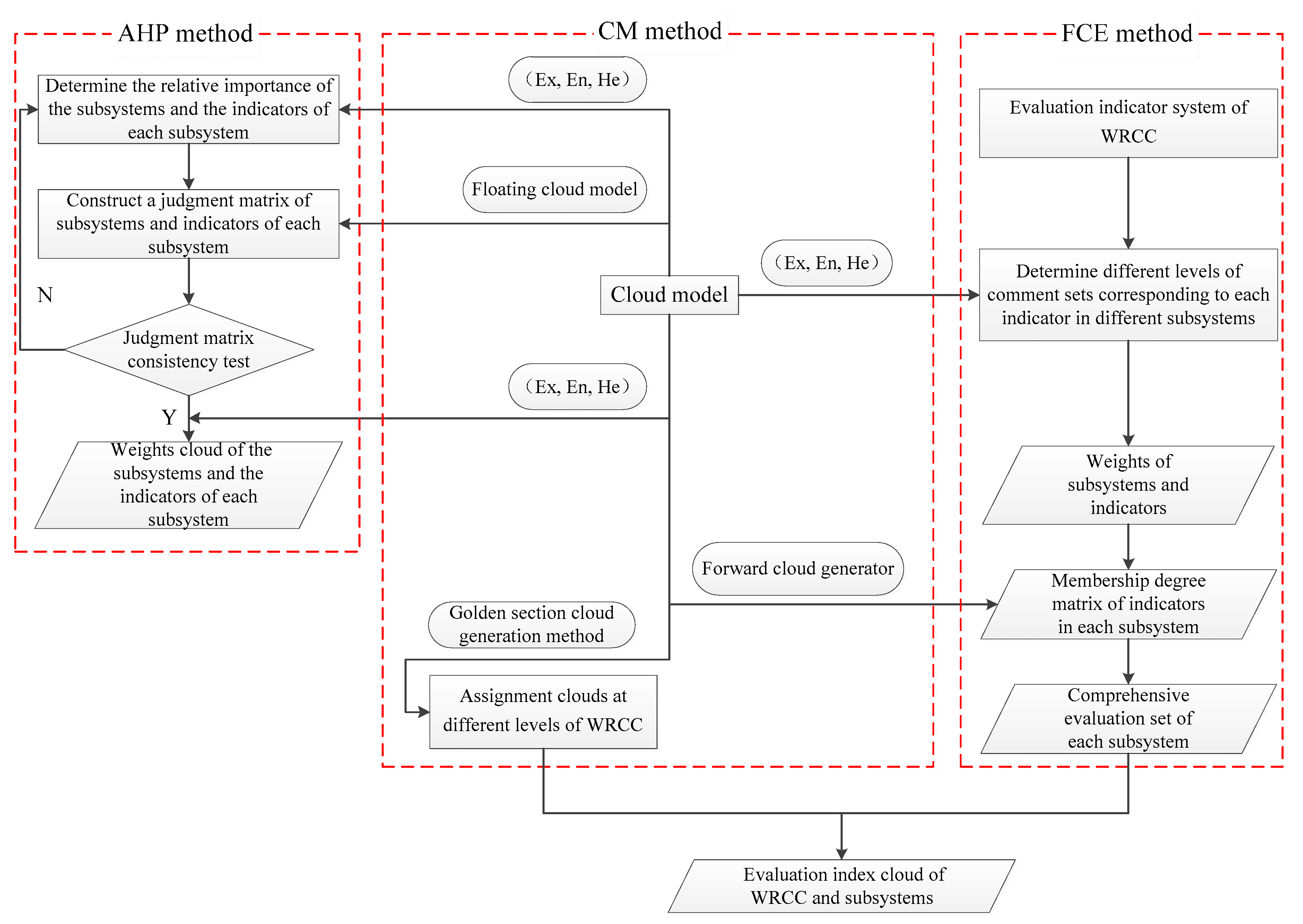
Figure 1. The theory and integration method of the proposed fuzzy comprehensive evaluation-analytical hierarchy process-cloud model (FCE-AHP-CM) hybrid approach for water resources carrying capacity assessment (WRCCA).
Water 12 03241 g001
Figure 2. The assignment clouds of WRCC levels.
Water 12 03241 g002
Figure 3. The geographical location and hydrometeorological conditions of the study area.
Water 12 03241 g003
Figure 4. Proportion of the water resources of Datong in 2017 according to different types.
Water 12 03241 g004
Figure 5. Proportion of the water resources of Datong in 2017 according to different usages.
Water 12 03241 g005
Figure 6. The evaluation index cloud for WRCCA of the study area in 2017.
Water 12 03241 g006
Figure 7. The WRCC evaluation index cloud of each subsystem of the study area in 2017. (a) Hydrology subsystem. (b) Water resources utilization subsystem. (c) Water ecological environment subsystem. (d) Economy and society subsystem.
Water 12 03241 g007
Figure 8. The calculated WRCC levels, evaluation indexes and the actual WRCC states of the study area from 1988 to 2017.
Water 12 03241 g008
Figure 9. The evaluation indexes of every subsystems and the comprehensive evaluation indexes of WRCC in the study area from 1988 to 2017.
Water 12 03241 g009
Table 1. The relative importance scales of influencing factors.
Relative ImportanceDegreeSaaty ScaleCloud Scale
i is more important than jExtreme9(9,0.17,0.05)
Strong7(7,0.17,0.05)
Obvious5(5,0.17,0.05)
A little3(3,0.17,0.05)
i is as important as jEqual1(1,0,0)
j is more important than iA little1/3(1/3,0.17/9,0.05/9)
Obvious1/5(1/5,0.17/25,0.05/25)
Strong1/7(1/7,0.17/49,0.05/49)
Extreme1/9(1/9,0.17/81,0.05/81)
i is more important than j, and the importance is between the two integers2, 4, 6, 8(2,0.17,0.05)
j is more important than i, and the importance is between the two reciprocals of integers1/2, 1/4, 1/6, 1/8(1/2,0.17/4,0.05/4)
Table 2. The average values of the consistency random indicators.
Order123456789101112131415
RI000.520.891.121.261.361.411.461.491.521.541.561.581.59
Order161718192021222324252627282930
RI1.59431.60641.61331.62071.62921.63851.64031.64621.64971.65561.65871.66311.6671.66931.6724
Table 3. The assignment cloud eigenvalues of water resources carrying capacity (WRCC) levels of each subsystem.
SubsystemD1D2D3D4D5
Hydrology (+)(0,0.515,0.065)(1.545,0.318,0.04)(2.5,0.2,0.02)(3.455,0.318,0.04)(5,0.515,0.065)
Water resources utilization (+)(0,0.515,0.065)(1.545,0.318,0.04)(2.5,0.2,0.02)(3.455,0.318,0.04)(5,0.515,0.065)
Water ecological environment (+)(0,0.515,0.065)(1.545,0.318,0.04)(2.5,0.2,0.02)(3.455,0.318,0.04)(5,0.515,0.065)
Economy and society (−)(5,0.515,0.065)(3.455,0.318,0.04)(2.5,0.2,0.02)(1.545,0.318,0.04)(0,0.515,0.065)
Table 4. The evaluation indicator system for WRCCA in the study area.
Target LayerSystem LayerIndicator LayerCalculation FormulaSignificance
Evaluation of WRCCHydrology (+)Precipitation in flood season (+)Measured dataReflect regional precipitation during the flood season
Runoff depth (+)Annual runoff/AreaReflects water depth evenly distributed over the area
Water resources per capita (+)Total water resources/Total populationReflecting the abundance, shortage, and potential of regional water resources
Water resources per unit area (+)Total water resources/AreaReflects water resources per unit area
Water production coefficient (+)Total water resources/PrecipitationReflects precipitation capacity in the research area
Drought Index (−)Evaporation/PrecipitationReflect the degree of regional drought
Water resources utilization (+)Water consumption per capita (−)Total water use/Total populationReflect per capita water use
Water supply modulus (−)Water supply/AreaReflecting water use per unit area
Development and utilization of surface water resources (−)Surface water supply/Surface water availabilityReflect the degree of exploitation and utilization of surface water resources
Average water consumption per hectare of farmland irrigation (−)Farmland irrigation water consumption/Irrigated areaReflecting water use efficiency of agricultural
Proportion of groundwater use (−)Groundwater consumption/Total water consumptionReflect the proportion of groundwater use
Groundwater exploitation efficient (−)Actual groundwater exploitation/Exploitable groundwaterReflect the status and potential of groundwater exploitation
Water consumption per ten-thousand CNY (USD 1426) of industrial added value (−)Industrial water consumption/Industrial added valueReflect industrial water utilization levels
Urban domestic water quota (−)Urban water consumption/Urban population/daysReflect the level of urban residents’ domestic water use
Rural domestic water quota (−)Rural water consumption/Rural population/daysReflect the level of rural residents’ domestic water use
Water consumption per ten-thousand CNY (USD 1426) of GDP (−)Total water consumption/GDPReflect the overall economic water situation in the region
Proportion of water used in the tertiary industry (+)Tertiary industry water consumption/Total water consumptionReflect the proportion of water used in the tertiary industry
Water ecological environment (+)Ecological environment water use rate (+)Ecological and environmental water consumption/Total water resourcesReflect ecosystem needs for water
Wastewater discharge per ten-thousand CNY (USD 1426) output value (−)Wastewater discharge/GDPReflecting the status of wastewater discharge
Wastewater utilization rate (+)Wastewater utilization/Wastewater dischargeReflecting wastewater utilization capacity
Dilution ratio (−)Wastewater discharge/Surface runoffReflect the surface water pollution status and dilution ability
Surface water quality index (+)Concentration percentage value of the indicators in the corresponding gradeReflect the quality of surface water environment
Economy and society (−)Population density (+)Total population/AreaReflect regional population scale
GDP per capita (+)GDP/Total populationReflect the overall economic level of the region
Urbanization rate (+)Urban population/Total populationReflect the scale of regional urban population
Tertiary industry ratio (+)Added value of tertiary industry/GDPReflect the status of regional tertiary industry structure
Annual GDP growth rate (+)(GDP of the current year-GDP of the previous year)/GDP of the previous yearReflect the overall economic development capacity of the region
Table 5. The level standards and data in 2017 of evaluation indicators for WRCCA of the study area.
IndicatorUnitValue in 2017The Maximum ValueThe Minimum ValueD1D2D3D4D5
Precipitation in flood seasonmm307.3520180<248(248, 316)(316, 384)(384, 452)≥452
Runoff depthmm347015<26(26, 37)(37, 48)(48, 59)≥59
Water resources per capitam3/person277.2480180<240(240, 300)(300, 360)(360, 420)≥420
Water resources per unit area104 m3/km26.8104<5.2(5.2, 6.4)(6.4, 7.6)(7.6, 8.8)≥8.8
Water production coefficient-0.20.250.1<0.13(0.13, 0.16)(0.16, 0.19)(0.19, 0.22)≥0.22
Drought Index-2.44.51.5≥3.9(3.3, 3.9)(2.7, 3.3)(2.1, 2.7)<2.1
Water consumption per capitam3/person178.7240120≥216(192, 216)(168, 192)(144, 168)<144
Water supply modulus104 m3/km24.45.52.5≥4.9(4.3, 4.9)(3.7, 4.3)(3.1, 3.7)<3.1
Development and utilization of surface water resources%679020≥76(62, 76)(48, 62)(34, 48)<34
Average water consumption per hectare of farmland irrigationm3/hm2161.2350150≥310(270, 310)(230, 270)(190, 230)<190
Proportion of groundwater use%54.17545≥69(63, 69)(57, 63)(51, 57)<51
Groundwater exploitation efficient-0.810.4≧0.88(0.76, 0.88)(0.64, 0.76)(0.52, 0.64)<0.52
Water consumption per ten-thousand CNY (USD 1426) of industrial added valuem3/104 CNY54.838050≥314(248, 314)(182, 248)(116, 182)<116
Urban domestic water quotaL/person.day82.814070≥126(112, 126)(98, 112)(84, 98)<84
Rural domestic water quotaL/person.day63.18030≥70(60, 70)(50, 60)(40, 50)<40
Water consumption per ten-thousand CNY (USD 1426) of GDPm3/104 CNY52.522040≥184(148, 184)(112, 148)(76, 112)<76
Proportion of water used in the tertiary industry%1.820.8<1.04(1.04, 1.28)(1.28, 1.52)(1.52, 1.76)≥1.76
Ecological environment water use rate%4.750.5<1.4(1.4, 2.3)(2.3, 3.2)(3.2, 4.1)≥4.1
Wastewater discharge per ten-thousand CNY (USD 1426) output valuem3/104 CNY9.21705≥137(104, 137)(71, 104)(38, 71)<38
Wastewater utilization rate%49.8505<14(14, 23)(23, 32)(32, 41)≥41
Dilution ratio%15.8305≥25(20, 25)(15, 20)(10, 15)<10
Surface water quality index-598020<32(32, 44)(44, 56)(56, 68)≥68
Population densityperson/km2244.2300190<212(212, 234)(234, 256)(256, 278)≥278
GDP per capita104 CNY/person2.450.5<1.4(1.4, 2.3)(2.3, 3.2)(3.2, 4.1)≥4.1
Urbanization rate%62.96520<29(29, 38)(38, 47)(47, 56)≥56
Tertiary industry ratio%475020<26(26, 32)(32, 38)(38, 44)≥44
Annual GDP growth rate%4.8102<3.6(3.6, 5.2)(5.2, 6.8)(6.8, 8.4)≥8.4
Table 6. The aggregated judgement matrix of subsystems.
SubsystemHydrologyWater Resources UtilizationWater Ecological EnvironmentEconomy and Society
1(1,0,0)(1.167,0.103,0.052)(1.443,0.158,0.070)(1.500,0.156,0.072)
2 (1,0,0)(1.167,0.103,0.052)(1.333,0.085,0.050)
3 (1,0,0)(1.333,0.085,0.050)
4 (1,0,0)
Table 7. The aggregated judgement matrix of indicators in hydrology subsystem.
IndicatorPrecipitation in Flood SeasonRunoff DepthWater Resources per CapitaWater Resources per Unit AreaWater Production CoefficientDrought Index
1(1,0,0)(1.667,0.136,0.071)(2.333,0.170,0.087)(3.667,0.170,0.087)(3.000,0.170,0.087)(4.667,0.170,0.087)
2 (1,0,0)(1.667,0.136,0.071)(3.000,0.170,0.087)(2.333,0.170,0.087)(4.000,0.170,0.087)
3 (1,0,0)(2.333,0.170,0.087)(1.667,0.136,0.071)(3.333,0.170,0.087)
4 (1,0,0)(0.600,0.024,0.018)(2.000,0.170,0.087)
5 (1,0,0)(2.667,0.170,0.087)
6 (1,0,0)
Table 8. The aggregated judgement matrix of indicators in water resources utilization subsystem.
IndicatorWater Consumption per CapitaWater Supply ModulusDevelopment and Utilization of Surface Water ResourcesAverage Water Consumption per Hectare of Farmland IrrigationProportion of Groundwater UseGroundwater Exploitation EfficientWater Consumption per ten-thousand CNY of Industrial Added ValueUrban Domestic Water QuotaRural Domestic Water QuotaWater Consumption per ten-thousand CNY of GDPProportion of water Used in the Tertiary Industry
1(1,0,0)(2.167,0.160,0.072)(0.750,0.009,0.013)(1,0,0)(3.333,0.170,0.087)(0.750,0.009,0.013)(1.444,0.158,0.071)(3.667,0.170,0.087)(5.667,0.170,0.087)(1.444,0.158,0.071)(4.667,0.170,0.087)
2 (1,0,0)(0.400,0.291,0.050)(0.462,0.255,0.051)(2.333,0.170,0.087)(0.400,0.291,0.050)(0.500,0.043,0.022)(2.667,0.170,0.087)(4.667,0.170,0.087)(0.500,0.043,0.022)(3.667,0.170,0.087)
3 (1,0,0)(1.333,0.085,0.050)(3.667,0.170,0.087)(1,0,0)(1.778,0.161,0.071)(4.000,0.170,0.087)(6.000,0.170,0.087)(1.778,0.161,0.071)(5.000,0.170,0.087)
4 (1,0,0)(3.333,0.170,0.087)(0.750,0.009,0.013)(1.444,0.158,0.071)(3.667,0.170,0.087)(5.667,0.170,0.087)(1.444,0.158,0.071)(4.667,0.170,0.087)
5 (1,0,0)(0.273,0.031,0.013)(0.300,0.017,0.008)(1.333,0.085,0.050)(3.333,0.170,0.087)(0.300,0.017,0.008)(2.333,0.170,0.087)
6 (1,0,0)(1.778,0.161,0.071)(4.000,0.170,0.087)(6.000,0.170,0.087)(1.778,0.161,0.071)(5.000,0.170,0.087)
7 (1,0,0)(3.667,0.170,0.087)(5.667,0.170,0.087)(1,0,0)(4.667,0.170,0.087)
8 (1,0,0)(3.000,0.170,0.087)(0.273,0.017,0.008)(2.000,0.170,0.087)
9 (1,0,0)(0.176,0.006,0.003)(0.500,0.043,0.022)
10 (1,0,0)(4.667,0.170,0.087)
11 (1,0,0)
Table 9. The aggregated judgement matrix of indicators in water ecological environment subsystem.
IndicatorEcological Environment Water Use RateWastewater Discharge per Ten-Thousand CNY Output ValueWastewater Utilization RateDilution RatioSurface Water Quality Index
1(1,0,0)(2.667,0.170,0.087)(3.000,0.170,0.087)(2.000,0.142,0.071)(0.667,0.191,0.053)
2 (1,0,0)(1.333,0.085,0.050)(0.600,0.024,0.018)(0.333,0.019,0.010)
3 (1,0,0)(0.500,0.043,0.022)(0.300,0.017,0.008)
4 (1,0,0)(0.429,0.038,0.019)
5 (1,0,0)
Table 10. The aggregated judgement matrix of indicators in economy and society subsystem.
IndicatorPopulation DensityGDP per CapitaUrbanization RateTertiary Industry RatioAnnual GDP Growth Rate
1(1,0,0)(0.857,0.140,0.052)(2.000,0.170,0.087)(3.000,0.170,0.087)(2.000,0.142,0.071)
2 (1,0,0)(2.000,0.142,0.071)(3.000,0.170,0.087)(2.000,0.170,0.087)
3 (1,0,0)(2.000,0.142,0.071)(0.857,0.140,0.052)
4 (1,0,0)(0.500,0.043,0.022)
5 (1,0,0)
Table 11. The weights clouds eigenvalues of each subsystem and indicator of the study area in 2017.
SubsystemWeight Cloud EigenvaluesIndicatorWeight Cloud Eigenvalues
Hydrology(0.310,0.285,0.305)Precipitation in flood season(0.336,0.339,0.336)
Runoff depth(0.241,0.229,0.235)
Water resources per capita(0.169,0.178,0.173)
Water resources per unit area(0.083,0.081,0.082)
Water production coefficient(0.118,0.124,0.122)
Drought Index(0.053,0.050,0.051)
Water resources utilization(0.264,0.250,0.262)Water consumption per capita(0.132,0.127,0.130)
Water supply modulus(0.072,0.081,0.077)
Development and utilization of surface water resources(0.160,0.152,0.157)
Average water consumption per hectare of farmland irrigation(0.132,0.127,0.130)
Proportion of groundwater use(0.043,0.042,0.043)
Groundwater exploitation efficient(0.160,0.152,0.157)
Water consumption per ten-thousand CNY of industrial added value(0.110,0.121,0.114)
Urban domestic water quota(0.037,0.035,0.036)
Rural domestic water quota(0.019,0.017,0.018)
Water consumption per ten-thousand CNY of GDP(0.110,0.121,0.114)
Proportion of water used in the tertiary industry(0.026,0.024,0.025)
Water ecological environment(0.233,0.265,0.243)Ecological environment water use rate(0.280,0.311,0.292)
Wastewater discharge per ten-thousand CNY output value(0.110,0.105,0.109)
Wastewater utilization rate(0.091,0.086,0.088)
Dilution ratio(0.163,0.157,0.163)
Surface water quality index(0.356,0.341,0.349)
Economy and society(0.193,0.200,0.190)Population density(0.289,0.299,0.293)
GDP per capita(0.307,0.300,0.304)
Urbanization rate(0.153,0.158,0.155)
Tertiary industry ratio(0.089,0.085,0.086)
Annual GDP growth rate(0.163,0.159,0.162)
Table 12. The eigenvalues of evaluation index clouds for WRCCA of the study area in 2017.
Name of the Evaluation Index CloudEigenvalues of the Cloud
Hydrology subsystem(2.006,0.162,0.160)
Water resources utilization subsystem(2.976,0.226,0.225)
Water ecological environment subsystem(3.944,0.386,0.389)
Economy and society subsystem(2.283,0.226,0.226)
Water resources carrying capacity(2.767,0.250,0.245)
Publisher’s Note: MDPI stays neutral with regard to jurisdictional claims in published maps and institutional affiliations.