An Optimized and Scalable Algorithm for the Fast Convergence of Steady 1-D Open-Channel Flows


Abstract
:1. Introduction
2. Materials and Methods
2.1. Equations
2.2. Original Solving Strategy
2.2.1. Non-Linear Krylov Acceleration
- The first term depicts the correction as a linear combination of previous corrections.
- The second term is similar to the second term of a fixed-point iteration that takes into account previous evolutions of function f.
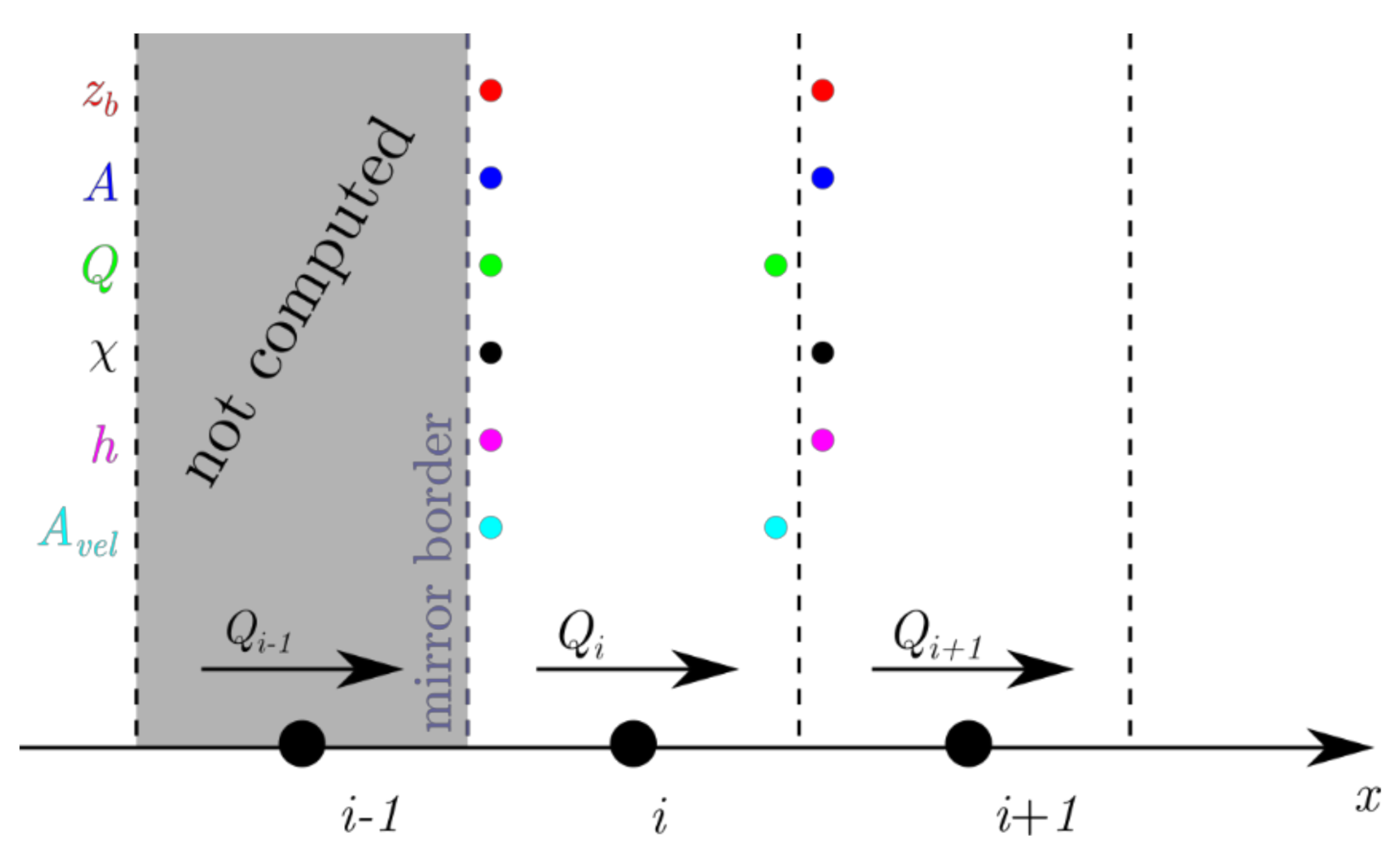
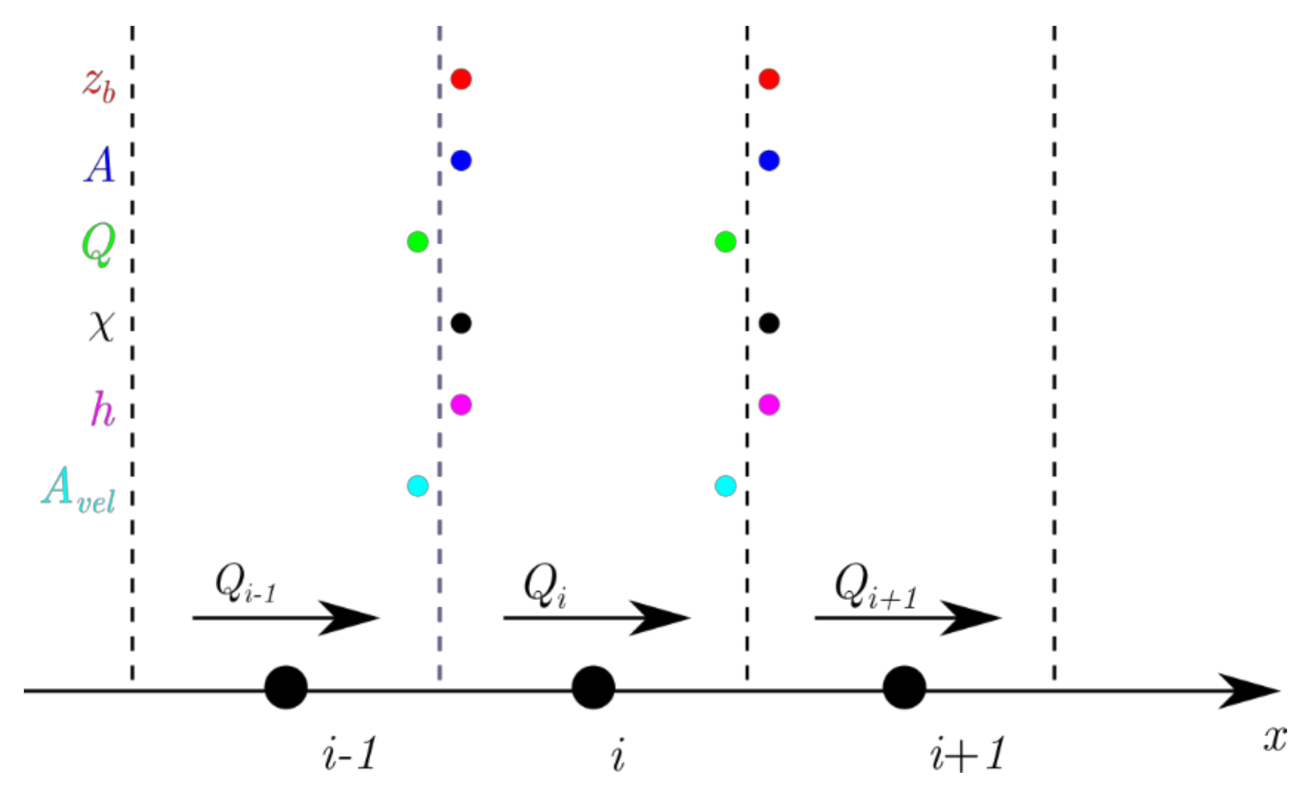
2.2.2. Evolutionary Domain
2.2.3. Combination of Solving Strategies
| Algorithm 1 |
| Initialize (computation list is empty) |
| Add most downstream node to computation list |
| While some nodes still have to be converged (): |
| Add most downstream node to computation list |
| Initialize lastly added upstream node |
| While nodes of computation list not converged (): |
| Compute cross section change for each node |
| If NKA activated: |
| Adapt cross section change with NKA algorithm |
| If lastly removed downstream node significantly impacted: |
| Add it back to the computation list and do not expand upstream |
| Else: |
| If downstream node in computation list fully converged (): |
| Remove this node from computation list |
| If upstream nodes remain to be added to computation list: |
| Add 1 upstream node to the computation list |
| Finalize |
2.3. Alternative Non-Linear Solver
3. Results and Discussion
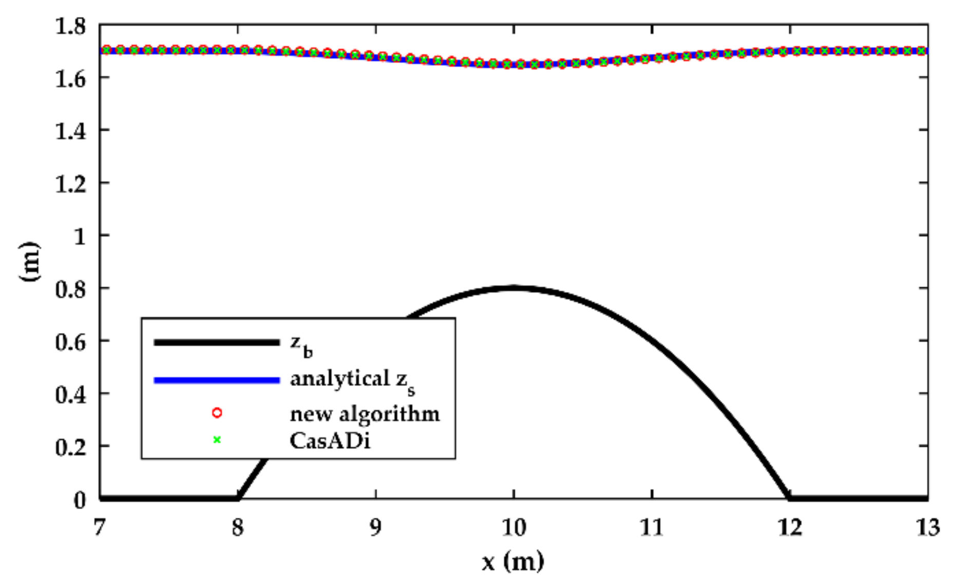
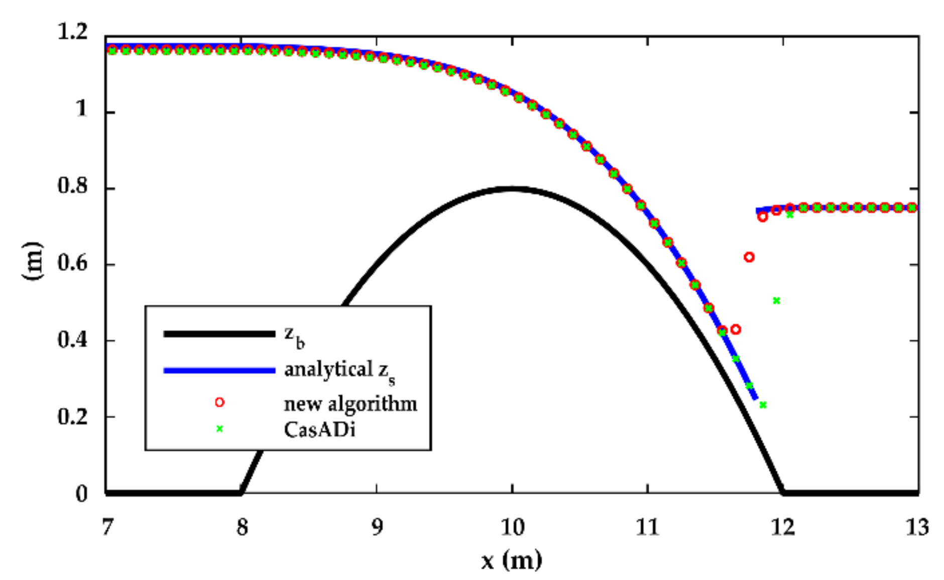
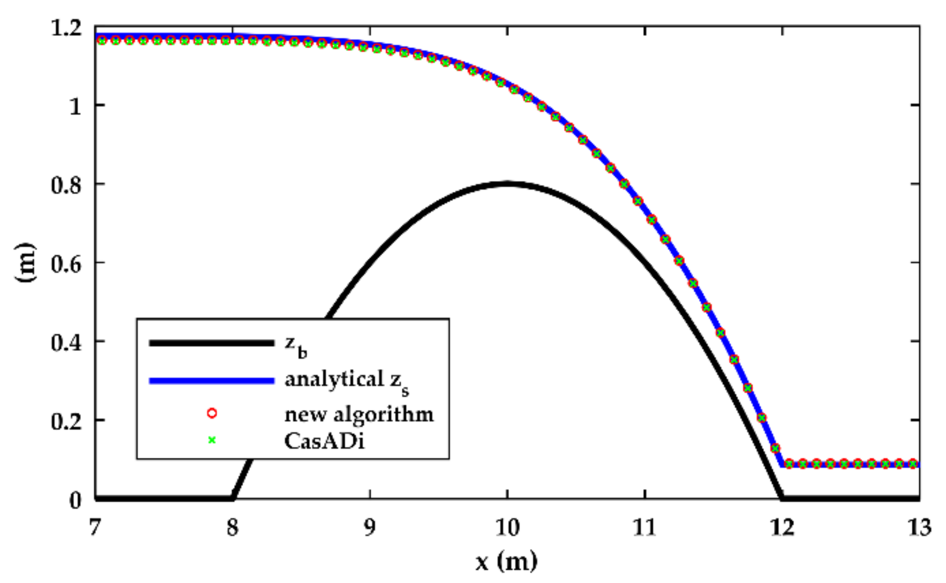
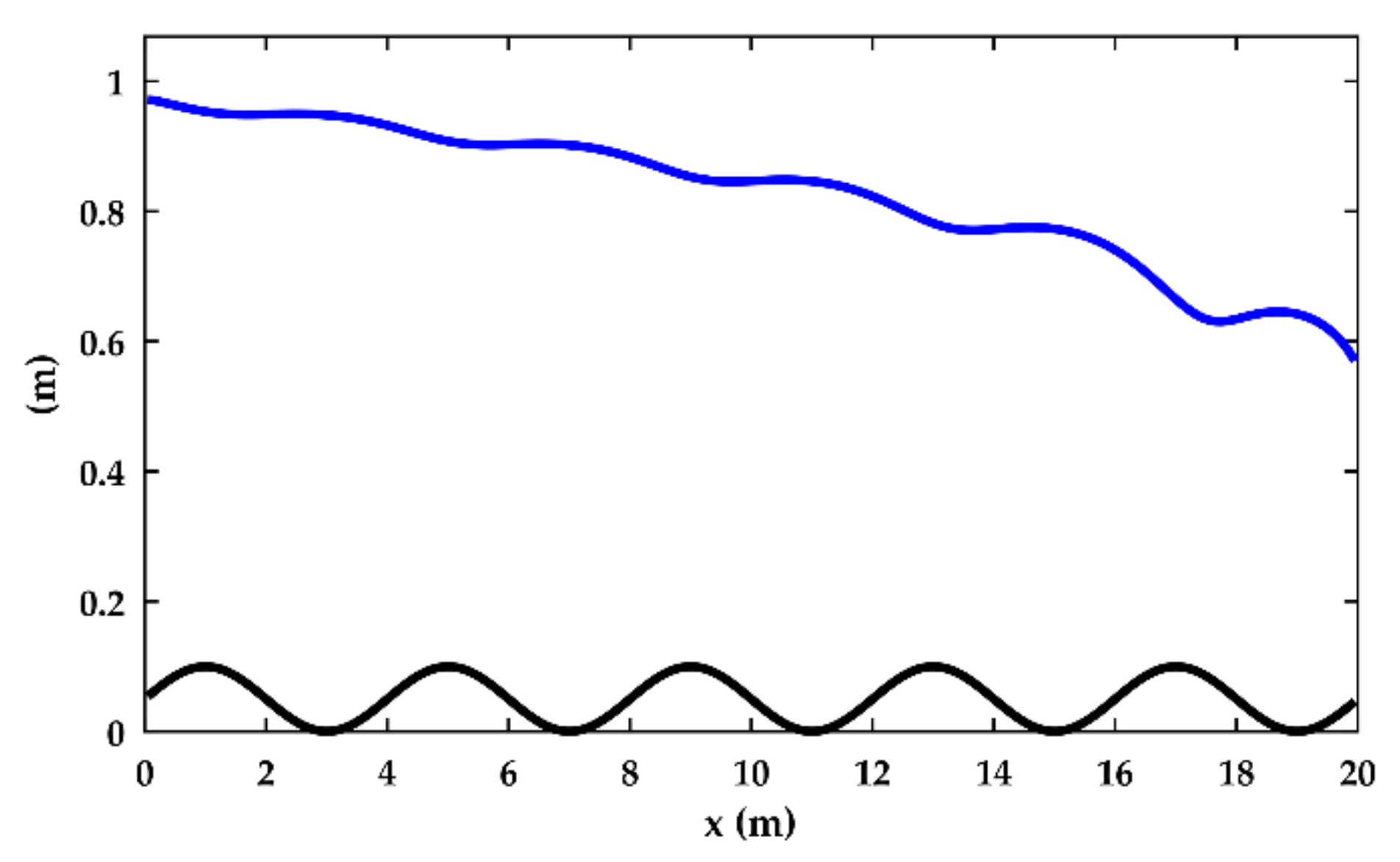
3.1. Validation
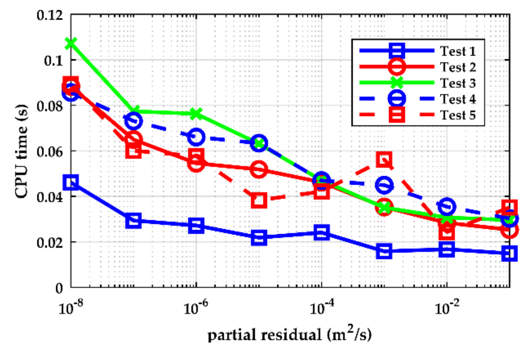
3.2. Optimal Setting of the New Algorithm
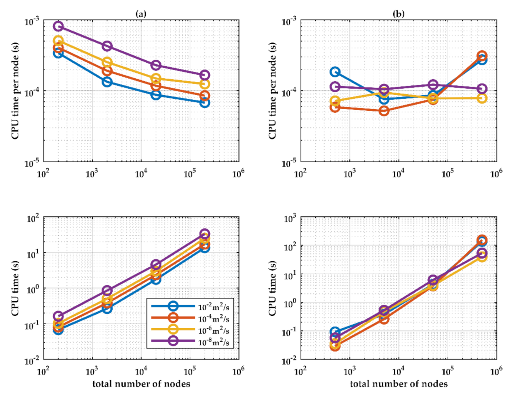
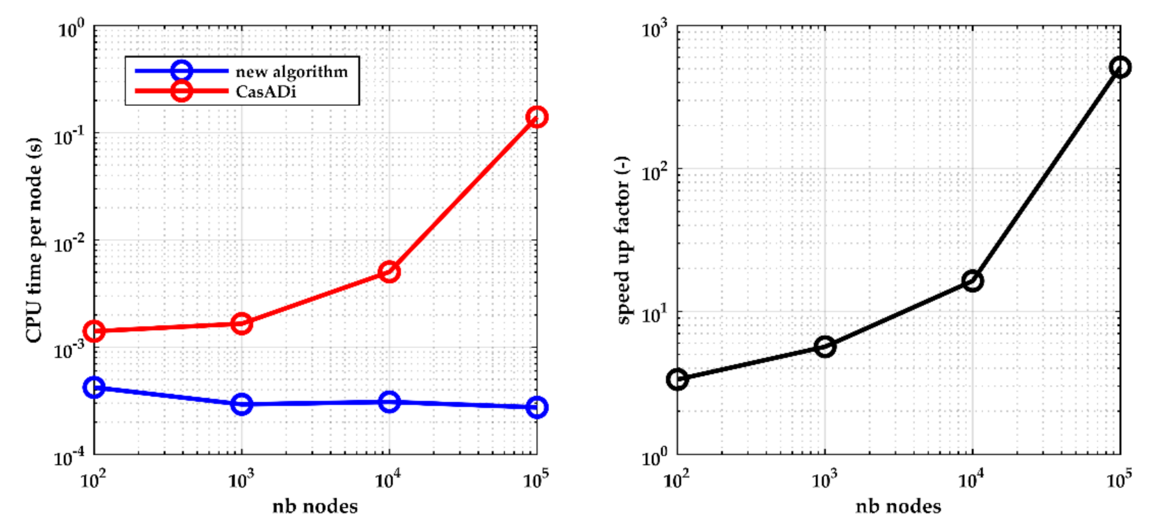
3.3. Performance of the Models
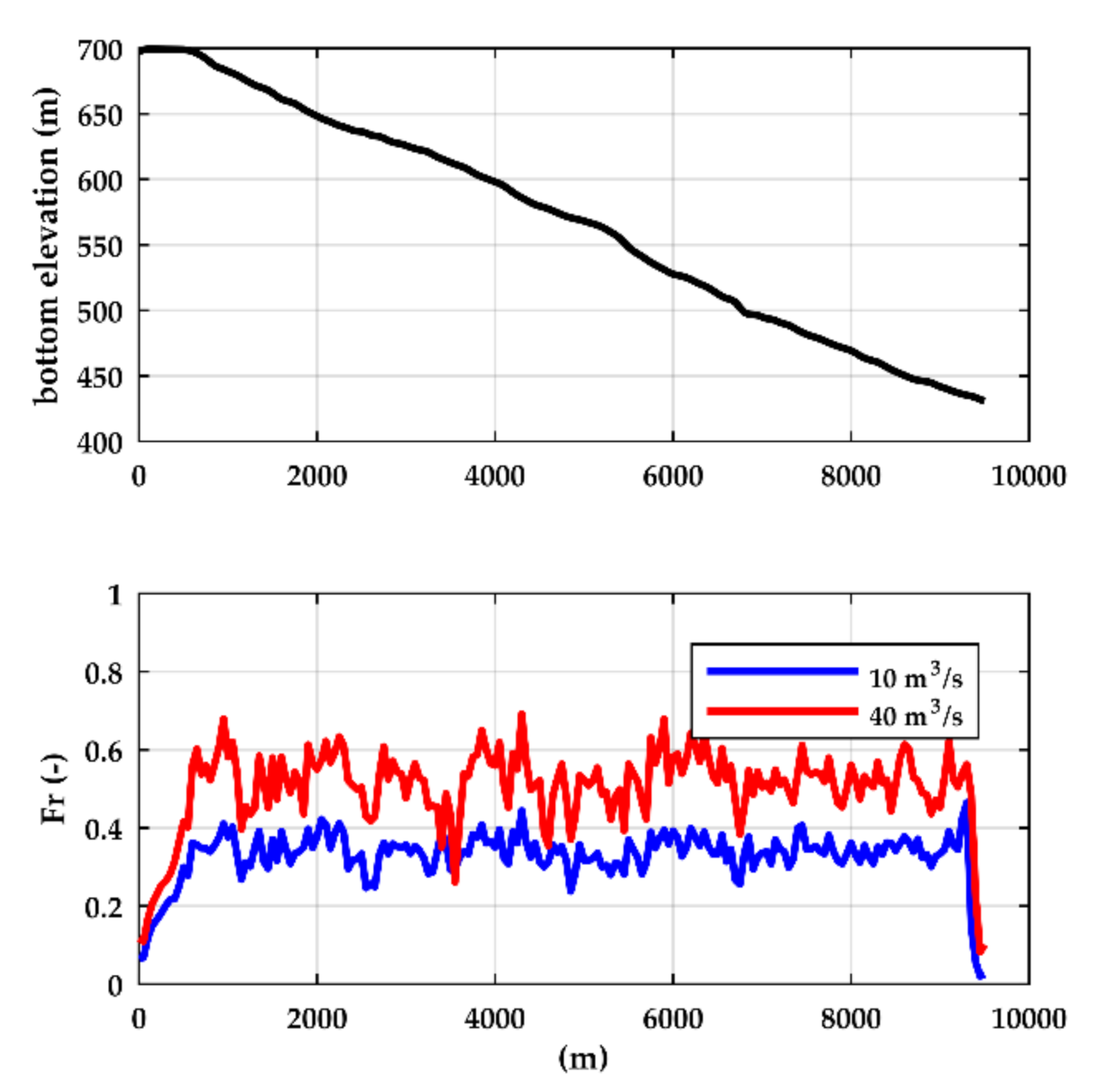
3.4. Real-World Application
4. Conclusions
Author Contributions
Funding
Conflicts of Interest
Computer Code and Software
References
- Proust, S.; Berni, C.; Boudou, M.; Chiaverini, A.; Dupuis, V.; Faure, J.-B.; Paquier, A.; Lang, M.; Guillen-Ludena, S.; Lopez, D.; et al. Predicting the flow in the floodplains with evolving land occupations during extreme flood events (FlowRes ANR project). In Proceedings of the E3S Web of Conferences, Lyon, France, 17–21 October 2016; Volume 7. [Google Scholar]
- Drab, A.; Riha, J. An approach to the implementation of European Directive 2007/60/EC on flood risk management in the Czech Republic. Nat. Hazards Earth Syst. Sci. 2010, 10, 1977–1987. [Google Scholar] [CrossRef]
- Schwanenberg, D.; Becker, B.P.J.; Xu, M. The open real-time control (RTC)-Tools software framework for modeling RTC in water resources sytems. J. Hydroinform. 2014, 17, 130–148. [Google Scholar] [CrossRef] [Green Version]
- Tayefi, V.; Lane, S.N.; Hardy, R.J.; Yu, D. A comparison of one- and two-dimensional approaches to modelling flood inundation over complex upland floodplains. Hydrol. Process. 2007, 21, 3190–3202. [Google Scholar] [CrossRef]
- Horritt, M.S.; Bates, P.D. Evaluation of 1D and 2D numerical models for predicting river flood inundation. J. Hydrol. 2002, 268, 87–99. [Google Scholar] [CrossRef]
- Cook, A.; Merwade, V. Effect of topographic data, geometric configuration and modeling approach on flood inundation mapping. J. Hydrol. 2009, 377, 131–142. [Google Scholar] [CrossRef]
- Goffin, L.; Dewals, B.J.; Erpicum, S.; Pirotton, M.; Archambeau, P. Non-linear optimization of a 1-D shallow water model and integration into Simulink for operational use. In Proceedings of the Sustainable Hydraulics in the Era of Global Change—4th European Congress of the International Association of Hydroenvironment Engineering and Research (IAHR 2016); Liege, Belgium, 27–29 July 2016, CRC Press/Balkema: Boca Raton, FL, USA, 2016; pp. 445–451. [Google Scholar]
- Bourdarias, C.; Gerbi, S.; Gisclon, M. A kinetic formulation for a model coupling free surface and pressurised flows in closed pipes. J. Comput. Appl. Math. 2008, 218, 522–531. [Google Scholar] [CrossRef] [Green Version]
- Paiva, R.C.D.; Collischonn, W.; Tucci, C.E.M. Large scale hydrologic and hydrodynamic modeling using limited data and a GIS based approach. J. Hydrol. 2011, 406, 170–181. [Google Scholar] [CrossRef]
- Paz, A.R.; Bravo, J.M.; Allasia, D.; Collischonn, W.; Tucci, C.E.M. Large-scale hydrodynamic modeling of a complex river network and floodplains. J. Hydrol. Eng. 2010, 15, 152–165. [Google Scholar] [CrossRef]
- Lai, X.; Jiang, J.; Liang, Q.; Huang, Q. Large-scale hydrodynamic modeling of the middle Yangtze River Basin with complex river-lake interactions. J. Hydrol. 2013, 492, 228–243. [Google Scholar] [CrossRef]
- Remo, J.W.F.; Pinter, N. Retro-modeling the Middle Mississippi River. J. Hydrol. 2007, 337, 421–435. [Google Scholar] [CrossRef]
- Biancamaria, S.; Bates, P.D.; Boone, A.; Mognard, N.M. Large-scale coupled hydrologic and hydraulic modelling of the Ob river in Siberia. J. Hydrol. 2009, 379, 136–150. [Google Scholar] [CrossRef] [Green Version]
- Kerger, F.; Archambeau, P.; Erpicum, S.; Dewals, B.J.; Pirotton, M. A fast universal solver for 1D continuous and discontinuous steady flows in rivers and pipes. Int. J. Numer. Methods Fluids 2011, 66, 38–48. [Google Scholar] [CrossRef]
- Sandric, I.; Ionita, C.; Chitu, Z.; Dardala, M.; Irimia, R.; Furtuna, F.T. Using CUDA to accelerate uncertainty propagation modelling for landslide susceptibility assessment. Environ. Model. Softw. 2019, 115, 176–186. [Google Scholar] [CrossRef]
- Neal, J.C.; Fewtrell, T.J.; Bates, P.D.; Wright, N.G. A comparison of three parallelisation methods for 2D flood inundation models. Environ. Model. Softw. 2010, 25, 398–411. [Google Scholar] [CrossRef]
- Lacasta, A.; Garcia-Navarro, P.; Burguete, J.; Murillo, J. Preprocess static subdomain decomposition in practical cases of 2D unsteady hydraulic simulation. Comput. Fluids 2013, 80, 225–232. [Google Scholar] [CrossRef] [Green Version]
- Brodtkorb, A.R.; Sætra, M.L.; Altinakar, M. Efficient shallow water simulations on GPUs: Implementation, visualization, verification, and validation. Comput. Fluids 2012, 55, 1–12. [Google Scholar] [CrossRef]
- Petaccia, G.; Leporati, F.; Torti, E. OpenMP and CUDA simulations of Sella Zerbino Dam break on unstructured grids. Comput. Geosci. 2016, 20, 1123–1132. [Google Scholar] [CrossRef]
- Smith, L.S.; Liang, Q. Towards a generalised GPU/CPU shallow-flow modelling tool. Comput. Fluids 2013, 88, 334–343. [Google Scholar] [CrossRef]
- Chaudhry, M.H. Open-Channel Flow; Springer Science & Business Media: Berlin/Heidelberg, Germany, 2007. [Google Scholar]
- Bruwier, M.; Archambeau, P.; Erpicum, S.; Pirotton, M.; Dewals, B. Discretization of the divergence formulation of the bed slope term in the shallow-water equations and consequences in terms of energy balance. Appl. Math. Model. 2016, 40, 7532–7544. [Google Scholar] [CrossRef]
- Franzini, F.; Soares-Frazão, S. Efficiency and accuracy of Lateralized HLL, HLLS and Augmented Roe’s scheme with energy balance for river flows in irregular channels. Appl. Math. Model. 2016, 40, 7427–7446. [Google Scholar] [CrossRef]
- Erpicum, S.; Dewals, B.; Archambeau, P.; Pirotton, M. Dam break flow computation based on an efficient flux vector splitting. J. Comput. Appl. Math. 2010, 234, 2143–2151. [Google Scholar] [CrossRef]
- Broyden, C.G. A class of methods for solving nonlinear simultaneous equations. Math. Comput. 1965, 19, 577–593. [Google Scholar] [CrossRef]
- Knoll, D.A.; Keyes, D.E. Jacobian-free Newton–Krylov methods: A survey of approaches and applications. J. Comput. Phys. 2004, 193, 357–397. [Google Scholar] [CrossRef] [Green Version]
- Anderson, D.G. Iterative Procedures for Nonlinear Integral Equations. J. ACM 1965, 12, 547–560. [Google Scholar] [CrossRef]
- Walker, H.F.; Ni, P. Anderson acceleration for fixed-point iterations. SIAM J. Numer. Anal. 2011, 49, 1715–1735. [Google Scholar] [CrossRef] [Green Version]
- Saad, Y.; Schultz, M.H. GMRES: A generalized minimal residual algorithm for solving nonsymmetric linear systems. SIAM J. Sci. Stat. Comput. 1986, 7, 856–869. [Google Scholar] [CrossRef] [Green Version]
- Carlson, N.N.; Miller, K. Design and application of a gradient-weighted moving finite element code I: In one dimension. SIAM J. Sci. Comput. 1998, 19, 728–765. [Google Scholar] [CrossRef]
- Carlson, N.N.; Miller, K. Design and Application of a Gradient-Weighted Moving Finite Element Code II: In Two Dimensions. SIAM J. Sci. Comput. 1998, 19, 766–798. [Google Scholar] [CrossRef] [Green Version]
- Calef, M.T.; Fichtl, E.D.; Warsa, J.S.; Berndt, M.; Carlson, N.N. Nonlinear Krylov acceleration applied to a discrete ordinates formulation of the k-eigenvalue problem. J. Comput. Phys. 2013, 238, 188–209. [Google Scholar] [CrossRef] [Green Version]
- Wang, C.; Cheng, J.; Berndt, M.; Carlson, N.N.; Luo, H. Application of nonlinear Krylov acceleration to a reconstructed discontinuous Galerkin method for compressible flows. Comput. Fluids 2018, 163, 32–49. [Google Scholar] [CrossRef]
- Andersson, J.A.E.; Gillis, J.; Horn, G.; Rawlings, J.B.; Diehl, M. CasADi—A software framework for nonlinear optimization and optimal control. Math. Program. Comput. 2018, 11, 1–36. [Google Scholar] [CrossRef]
- Baayen, J.; Piovesan, T.; VanderWees, J. Optimization problems subject to the nonlinear semi-implicitly discretized Saint-Venant equations have a unique solution. arXiv 2018, arXiv:1801.06507. [Google Scholar]
- Aureli, F.; Maranzoni, A.; Mignosa, P.; Ziveri, C. A weighted surface-depth gradient method for the numerical integration of the 2D shallow water equations with topography. Adv. Water Resour. 2008, 31, 962–974. [Google Scholar] [CrossRef]


| Test | Upstream BC | Downstream BC |
|---|---|---|
| A | q = 1 m2/s | h = 1.7 m |
| B | q = 0.4 m2/s | h = 0.75 m |
| C | q = 0.4 m2/s | Transmissive |
| Test | Analytical | New Algorithm | CasADi | ||
|---|---|---|---|---|---|
| Head (m) | Head (m) | Diff. | Head (m) | Diff. | |
| A | 1.71764 | 1.72147 | 0.22% | 1.71958 | 0.11% |
| B | 1.18040 | 1.17062 | −0.83% | 1.16664 | −1.17% |
| C | 1.18040 | 1.17062 | −0.83% | 1.16664 | −1.17% |
| Test | Channel Bed | Friction | BC |
|---|---|---|---|
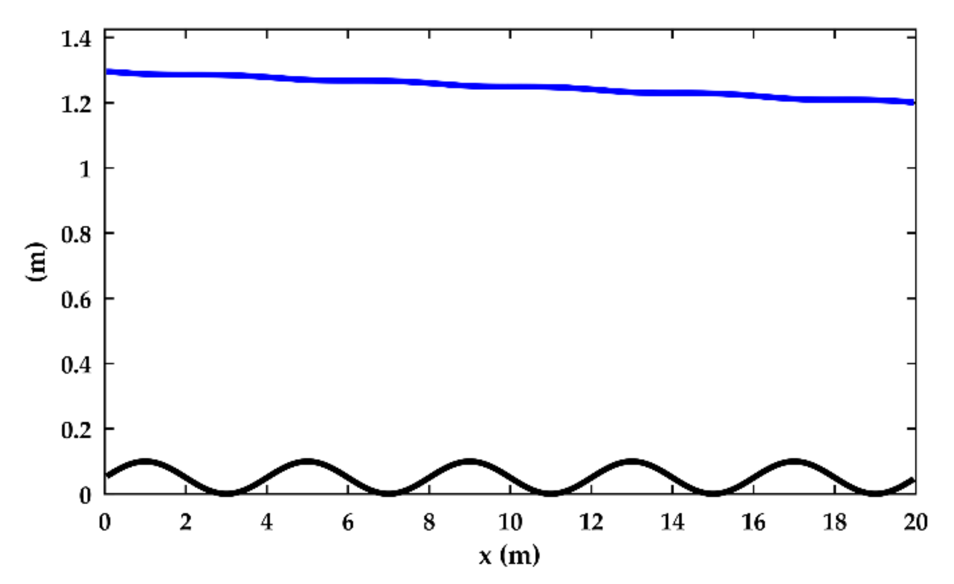
| 1 | , rectangular cross-section | Manning, n = 0.04 s/m1/3 | q = 1 m/s2, zdown = 1.2 m |
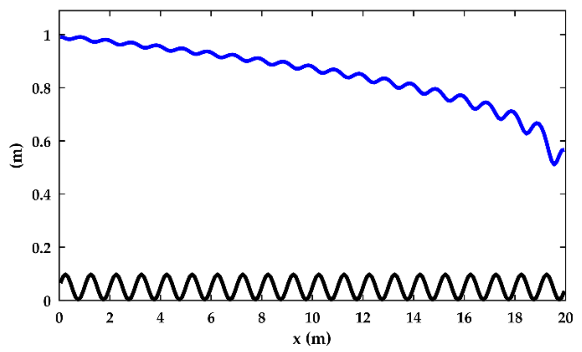
| 2 | , rectangular cross-section | Manning, n = 0.04 s/m1/3 | q = 1 m/s2, zdown = 0.55 m |
| 3 | , rectangular cross-section | Manning, n = 0.04 s/m1/3 | q = 1 m/s2, zdown = 0.55 m |
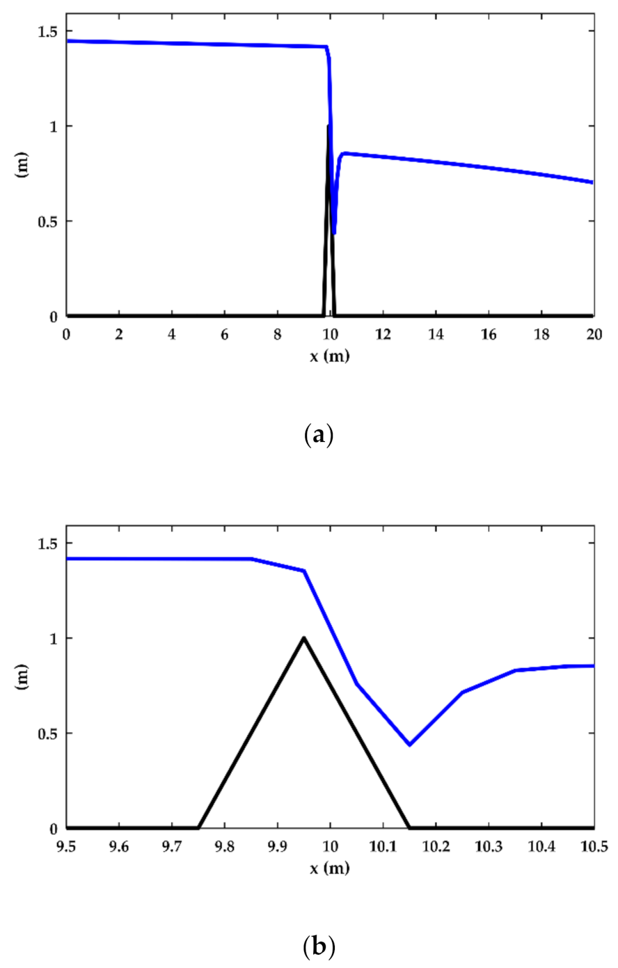
| 4 | Flat bottom with a weir, rectangular cross-section | Manning, n = 0.04 s/m1/3 | q = 1 m/s2, zdown = 0.7 m |
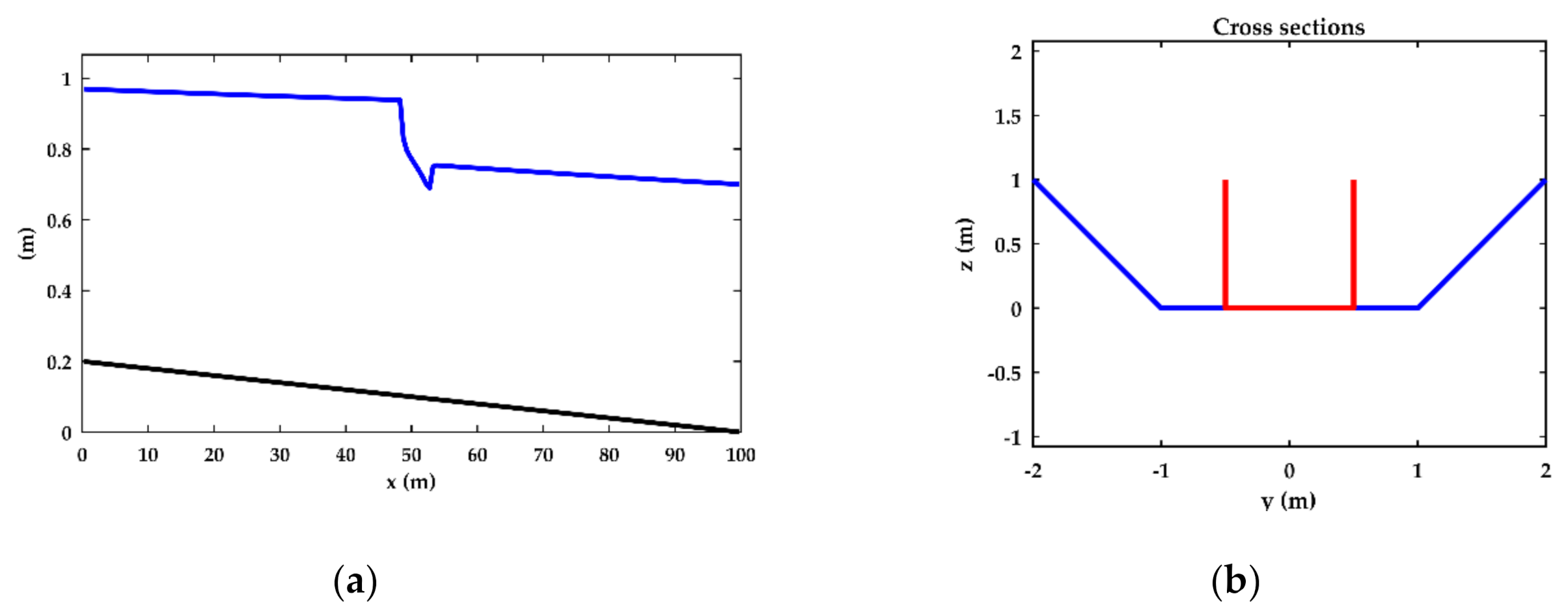
| 5 | 0.2% slope, sudden change in cross-section | Manning, n = 0.04 s/m1/3 | q = 1 m/s2, zdown = 0.7 m |
Publisher’s Note: MDPI stays neutral with regard to jurisdictional claims in published maps and institutional affiliations. |
© 2020 by the authors. Licensee MDPI, Basel, Switzerland. This article is an open access article distributed under the terms and conditions of the Creative Commons Attribution (CC BY) license (http://creativecommons.org/licenses/by/4.0/).
Share and Cite
Goffin, L.; Dewals, B.; Erpicum, S.; Pirotton, M.; Archambeau, P. An Optimized and Scalable Algorithm for the Fast Convergence of Steady 1-D Open-Channel Flows. Water 2020, 12, 3218. https://doi.org/10.3390/w12113218
Goffin L, Dewals B, Erpicum S, Pirotton M, Archambeau P. An Optimized and Scalable Algorithm for the Fast Convergence of Steady 1-D Open-Channel Flows. Water. 2020; 12(11):3218. https://doi.org/10.3390/w12113218
Chicago/Turabian StyleGoffin, Louis, Benjamin Dewals, Sebastien Erpicum, Michel Pirotton, and Pierre Archambeau. 2020. "An Optimized and Scalable Algorithm for the Fast Convergence of Steady 1-D Open-Channel Flows" Water 12, no. 11: 3218. https://doi.org/10.3390/w12113218
APA StyleGoffin, L., Dewals, B., Erpicum, S., Pirotton, M., & Archambeau, P. (2020). An Optimized and Scalable Algorithm for the Fast Convergence of Steady 1-D Open-Channel Flows. Water, 12(11), 3218. https://doi.org/10.3390/w12113218