Numerical Reconstruction of Three Holocene Glacial Events in Qiangyong Valley, Southern Tibetan Plateau and Their Implication for Holocene Climate Changes

Abstract
1. Introduction
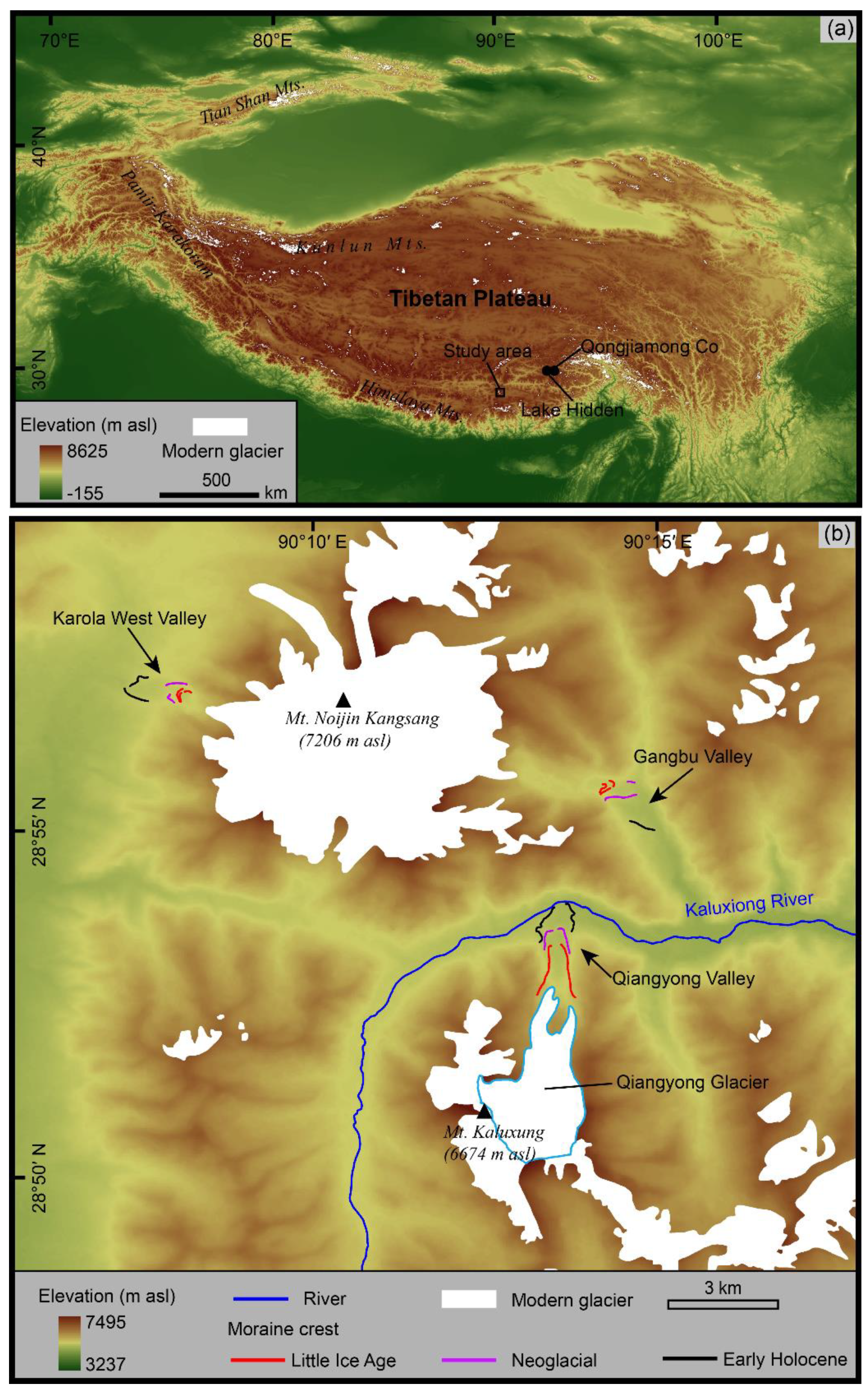
2. Study Area
3. Materials and Methods
3.1. Derivation of Glacier Bed Topography
3.2. Reconstruction of Paleo-Glacier Surface
3.3. Reconstruction of Paleoglacier ELA and Paleoclimate
4. Results and Discussion
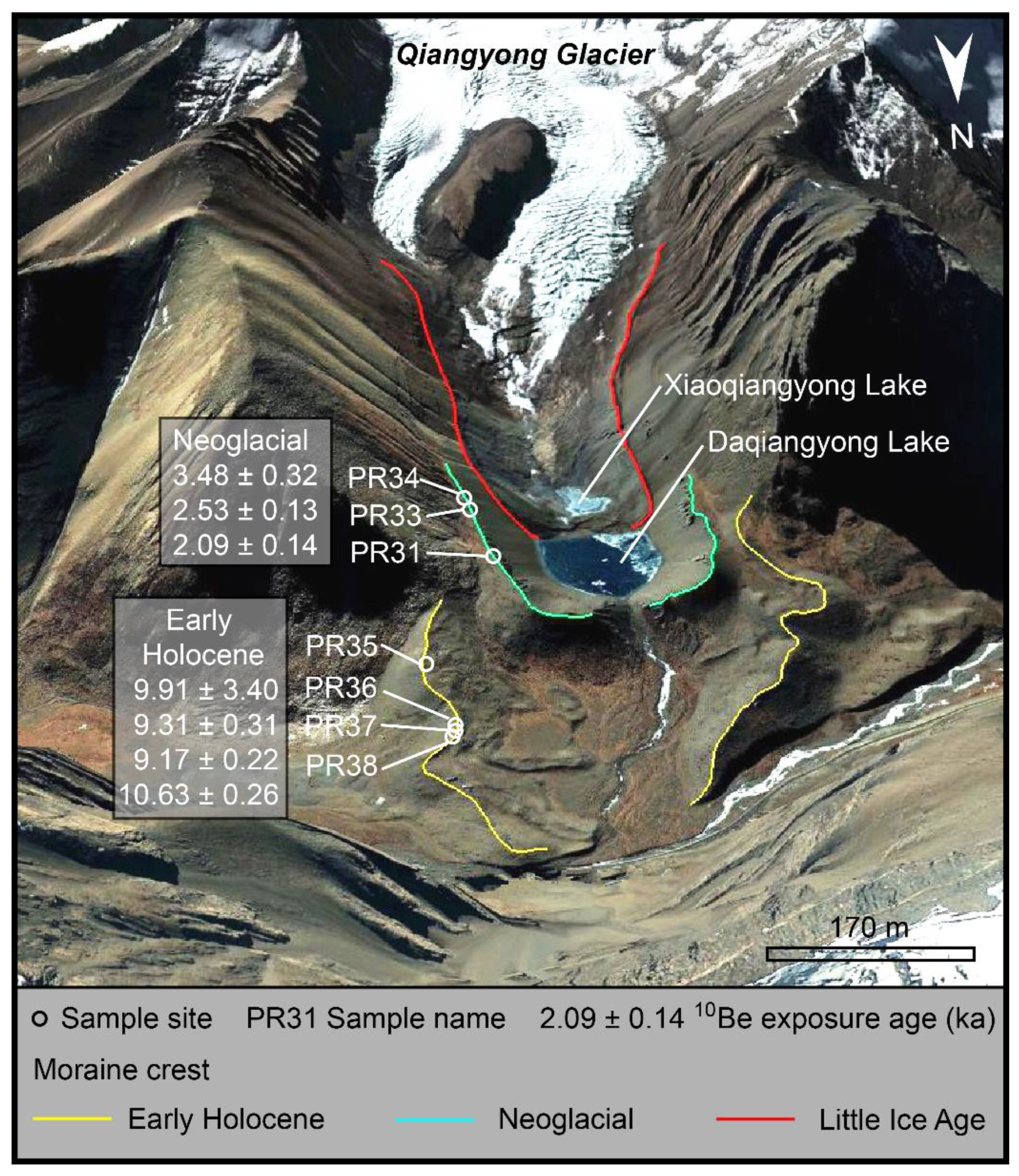
4.1. Glacier Extents of the Three Holocene Glacial Periods
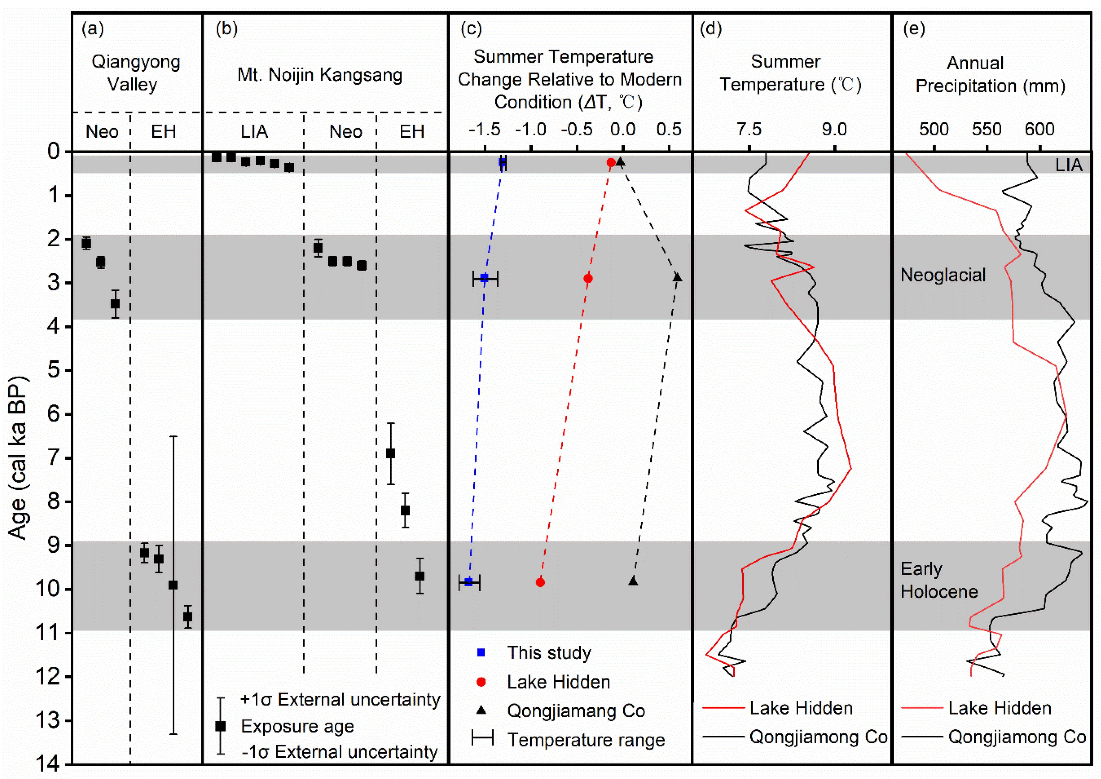
4.2. Climate Implications of the Three Glacial Events
5. Conclusions
Supplementary Materials
Author Contributions
Funding
Conflicts of Interest
References
- IPCC. The Physical Science Basis. Contribution of Working Group I to the Fifth Assessment Report of the Intergovernmental Panel on Climate Change; Cambridge University Press: Cambridge, UK, 2013. [Google Scholar] [CrossRef]
- Cuffey, K.M.; Paterson, W.S.B. The Physics of Glaciers, 4th ed.; Butterworth-Heinemann/Elsevier: Boston, MA, USA, 2010. [Google Scholar]
- Shi, Y. Characteristics of late Quaternary monsoonal glaciation on the Tibetan Plateau and in East Asia. Quatern. Int. 2002, 97–98, 79–91. [Google Scholar] [CrossRef]
- Thackray, G.D.; Owen, L.A.; Yi, C. Timing and nature of late Quaternary mountain glaciation. J. Quat. Sci. 2008, 23, 503–508. [Google Scholar] [CrossRef]
- Owen, L.A.; Caffee, M.W.; Finkel, R.C.; Seong, Y.B. Quaternary glaciation of the Himalayan-Tibetan orogen. J. Quat. Sci. 2008, 23, 513–531. [Google Scholar] [CrossRef]
- Owen, L.A. Latest Pleistocene and Holocene glacier fluctuations in the Himalaya and Tibet. Quat. Sci. Rev. 2009, 28, 2150–2164. [Google Scholar] [CrossRef]
- Zhou, S.; Chen, F.; Pan, B.; Cao, J.; Li, J.; Derbyshire, E. Environmental change during the Holocene in western China on a millennial timescale. Holocene 1991, 1, 151–156. [Google Scholar] [CrossRef]
- Yi, C.; Chen, H.; Yang, J.; Liu, B.; Fu, P.; Liu, K.; Li, S. Review of Holocene glacial chronologies based on radiocarbon dating in Tibet and its surrounding mountains. J. Quat. Sci. 2008, 23, 533–543. [Google Scholar] [CrossRef]
- Thompson, L.G.; Yao, T.; Davis, M.E.; Henderson, K.A.; Mosley-Thompson, E.; Lin, P.-N.; Beer, J.; Synal, H.-A.; Cole-Dai, J.; Bolzan, J.F. Tropical Climate Instability, The Last Glacial Cycle from a Qinghai-Tibetan Ice Core. Science 1997, 276, 1821–1825. [Google Scholar] [CrossRef]
- Seong, Y.B.; Owen, L.A.; Yi, C.; Finkel, R.C. Quaternary glaciation of Muztag Ata and Kongur Shan: Evidence for glacier response to rapid climate changes throughout the Late Glacial and Holocene in westernmost Tibet. Geol. Soc. Am. Bull. 2009, 121, 348–365. [Google Scholar] [CrossRef]
- Bond, G.; Kromer, B.; Beer, J.; Muscheler, R.; Evans, M.N.; Showers, W.; Hoffmann, S.; Lotti-Bond, R.; Hajdas, I.; Bonani, G. Persistent solar influence on North Atlantic climate during the Holocene. Science 2001, 294, 2130–2136. [Google Scholar] [CrossRef]
- Thompson, L.G.; Mosley-Thompson, E.; Davis, M.E.; Bolzan, J.F.; Dai, J.; Klein, L.; Yao, T.; Wu, X.; Xie, Z.; Gundestrup, N. Holocene--late pleistocene climatic ice core records from qinghai-tibetan plateau. Science 1989, 246, 474–477. [Google Scholar] [CrossRef]
- Owen, L.A.; Dortch, J.M. Nature and timing of Quaternary glaciation in the Himalayan–Tibetan orogen. Quat. Sci. Rev. 2014, 88, 14–54. [Google Scholar] [CrossRef]
- Finkel, R.C.; Owen, L.A.; Barnard, P.L.; Caffee, M.W. Beryllium-10 dating of Mount Everest moraines indicates a strong monsoon influence and glacial synchroneity throughout the Himalaya. Geology 2003, 31, 561–564. [Google Scholar] [CrossRef]
- Yang, J.; Zhang, W.; Cui, Z.; Yi, C.; Liu, K.; Ju, Y.; Zhang, X. Late Pleistocene glaciation of the Diancang and Gongwang Mountains, southeast margin of the Tibetan plateau. Quatern. Int. 2006, 154–155, 52–62. [Google Scholar] [CrossRef]
- Xu, X.; Yi, C. Little Ice Age on the Tibetan Plateau and its bordering mountains: Evidence from moraine chronologies. Glob. Planet Chang. 2014, 116, 41–53. [Google Scholar] [CrossRef]
- Saha, S.; Owen, L.A.; Orr, E.N.; Caffee, M.W. High-frequency Holocene glacier fluctuations in the Himalayan-Tibetan orogen. Quat. Sci. Rev. 2019, 220, 372–400. [Google Scholar] [CrossRef]
- Owen, L.A.; Finkel, R.C.; Barnard, P.L.; Ma, H.; Asahi, K.; Caffee, M.W.; Derbyshire, E. Climatic and topographic controls on the style and timing of Late Quaternary glaciation throughout Tibet and the Himalaya defined by 10Be cosmogenic radionuclide surface exposure dating. Quat. Sci. Rev. 2005, 24, 1391–1411. [Google Scholar] [CrossRef]
- Liu, J.; Yi, C.; Li, Y.; Bi, W.; Zhang, Q.; Hu, G. Glacial fluctuations around the Karola Pass, eastern Lhagoi Kangri Range, since the Last Glacial Maximum. J. Quat. Sci. 2017, 32, 516–527. [Google Scholar] [CrossRef]
- Li, J.; Zheng, B.; Yang, X. Glaciers in Tibet; Science Press: Beijing, China, 1986. [Google Scholar]
- Zhang, F.; Zhang, H.; Hagen, S.C.; Ye, M.; Wang, D.; Gui, D.; Zeng, C.; Tian, L.; Liu, J. Snow cover and runoff modelling in a high mountain catchment with scarce data: Effects of temperature and precipitation parameters. Hydrol. Process 2015, 29, 52–65. [Google Scholar] [CrossRef]
- Zheng, B. The influence of Himalayan uplift on the development of Quaternary glaciers. Z Geomorphol. 1989, 76, 89–115. [Google Scholar]
- James, W.H.M.; Carrivick, J.L. Automated modelling of spatially-distributed glacier ice thickness and volume. Comput. Geosci-UK 2016, 92, 90–103. [Google Scholar] [CrossRef]
- RGI Consortium. Randolph Glacier Inventory—A Dataset of Global Glacier Outlines: Version 6.0: Technical Report. Glob. Land Ice Meas. Space 2017. [Google Scholar] [CrossRef]
- Driedger, C.L.; Kennard, P.M. Glacier volume estimation on Cascade volcanoes: An analysis and comparison with other methods. Ann. Glaciol. 1986, 8, 59–64. [Google Scholar] [CrossRef]
- Nye, J.F. A method of calculating the thicknesses of the ice-sheets. Nature 1952, 169, 529–530. [Google Scholar] [CrossRef]
- Nye, J.F. The mechanics of glacier flow. J. Glaciol. 1952, 2, 82–93. [Google Scholar] [CrossRef]
- Pellitero, R.; Rea, B.R.; Spagnolo, M.; Bakke, J.; Ivy-Ochs, S.; Frew, C.R.; Hughes, P.; Ribolini, A.; Lukas, S.; Renssen, H. GlaRe, a GIS tool to reconstruct the 3D surface of palaeoglaciers. Comput. Geosci-UK 2016, 94, 77–85. [Google Scholar] [CrossRef]
- Benn, D.I.; Hulton, N.R.J. An ExcelTM spreadsheet program for reconstructing the surface profile of former mountain glaciers and ice caps. Comput. Geosci-UK 2010, 36, 605–610. [Google Scholar] [CrossRef]
- Van Der Veen, C.J. Fundamentals of Glacier Dynamics, 2nd ed.; Balkema: Rotterdam, The Netherlands, 2013. [Google Scholar]
- Porter, S.C. Equilibrium line altitudes of late Quaternary glaciers in the Southern Alps, New Zealand. Quat. Res. 1975, 5, 27–47. [Google Scholar] [CrossRef]
- Benn, D.I.; Owen, L.A.; Osmaston, H.A.; Seltzer, G.O.; Porter, S.C.; Mark, B. Reconstruction of equilibrium-line altitudes for tropical and sub-tropical glaciers. Quatern. Int. 2005, 138–139, 8–21. [Google Scholar] [CrossRef]
- Osmaston, H. Estimates of glacier equilibrium line altitudes by the Area×Altitude, the Area×Altitude Balance Ratio and the Area×Altitude Balance Index methods and their validation. Quatern. Int. 2005, 138–139, 22–31. [Google Scholar] [CrossRef]
- Dyurgerov, M.; Meier, M.F.; Bahr, D.B. A new index of glacier area change: A tool for glacier monitoring. J. Glaciol. 2009, 55, 710–716. [Google Scholar] [CrossRef]
- Rea, B.R. Defining modern day Area-Altitude Balance Ratios (AABRs) and their use in glacier-climate reconstructions. Quat. Sci. Rev. 2009, 28, 237–248. [Google Scholar] [CrossRef]
- Pellitero, R.; Rea, B.R.; Spagnolo, M.; Bakke, J.; Hughes, P.; Ivy-Ochs, S.; Lukas, S.; Ribolini, A. A GIS tool for automatic calculation of glacier equilibrium-line altitudes. Comput. Geosci-UK 2015, 82, 55–62. [Google Scholar] [CrossRef]
- Ohmura, A.; Kasser, P.; Funk, M. Climate at the Equilibrium Line of Glaciers. J. Glaciol. 1992, 38, 397–411. [Google Scholar] [CrossRef]
- Yao, T.; Thompson, L.; Yang, W.; Yu, W.; Gao, Y.; Guo, X.; Yang, X.; Duan, K.; Zhao, H.; Xu, B.; et al. Different glacier status with atmospheric circulations in Tibetan Plateau and surroundings. Nat. Clim. Chang. 2012, 2, 663–667. [Google Scholar] [CrossRef]
- Yao, T. Dataset of typical glacier changes on Tibetan Plateau and Its surrounding areas (2005–2016). Natl. Tibetan Plateau Data Cent. 2018. [Google Scholar] [CrossRef]
- Chen, F.; Zhang, J.; Liu, J.; Cao, X.; Hou, J.; Zhu, L.; Xu, X.; Liu, X.; Wang, M.; Wu, D.; et al. Climate change, vegetation history, and landscape responses on the Tibetan Plateau during the Holocene: A comprehensive review. Quat. Sci. Rev. 2020, 243, 1–21. [Google Scholar] [CrossRef]
- Balco, G.; Stone, J.O.; Lifton, N.A.; Dunai, T.J. A complete and easily accessible means of calculating surface exposure ages or erosion rates from 10Be and 26Al measurements. Quat. Geochronol. 2008, 3, 174–195. [Google Scholar] [CrossRef]
- Balco, G. Glacier change and paleoclimate applications of Cosmogenic-nuclide exposure dating. Annu. Rev. Earth Planet Sci. 2020, 48, 21–48. [Google Scholar] [CrossRef]
- Birks, H.J.B. Numerical tools in palaeolimnology–Progress, potentialities, and problems. J. Paleolimnol. 1998, 20, 307–332. [Google Scholar] [CrossRef]


| Glacial Stage | Area (km2) | Volume (m3) | Length (km) | Maximum Ice Thickness (m) | Average Ice Thickness (m) |
|---|---|---|---|---|---|
| Modern | 6.25 | 3.0 × 10⁸ | 4.7 | ~155 | ~47 |
| Little Ice Age | 7.68 | 4.6 × 10⁸ | 5.7 | ~223 | ~60 |
| Neoglacial | 8.45 | 6.2 × 10⁸ | 6.1 | ~246 | ~73 |
| Early Holocene | 10.00 | 8.1 × 10⁸ | 6.8 | ~268 | ~83 |
| Method | R/BR Value | Modern | Little Ice Age | Neoglacial | Early Holocene | Error # |
|---|---|---|---|---|---|---|
| AAR | 0.50 | 6100 | 5935 | 5927 | 5919 | ±25 |
| 0.60 | 5950 | 5835 | 5777 | 5769 | ±25 | |
| 0.65 | 5900 | 5735 | 5677 | 5669 | ±25 | |
| 0.70 | 5850 | 5635 | 5577 | 5519 | ±25 | |
| 0.80 | 5700 | 5435 | 5377 | 5319 | ±25 | |
| AABR | 1.04 | 6000 | 5835 | 5827 | 5769 | ±25 |
| 1.75 | 5900 | 5735 | 5687 | 5669 | ±25 | |
| 2.46 | 5850 | 5685 | 5637 | 5569 | ±25 |
Publisher’s Note: MDPI stays neutral with regard to jurisdictional claims in published maps and institutional affiliations. |
© 2020 by the authors. Licensee MDPI, Basel, Switzerland. This article is an open access article distributed under the terms and conditions of the Creative Commons Attribution (CC BY) license (http://creativecommons.org/licenses/by/4.0/).
Share and Cite
Sun, Y.; Xu, X.; Zhang, L.; Liu, J.; Zhang, X.; Li, J.; Pan, B. Numerical Reconstruction of Three Holocene Glacial Events in Qiangyong Valley, Southern Tibetan Plateau and Their Implication for Holocene Climate Changes. Water 2020, 12, 3205. https://doi.org/10.3390/w12113205
Sun Y, Xu X, Zhang L, Liu J, Zhang X, Li J, Pan B. Numerical Reconstruction of Three Holocene Glacial Events in Qiangyong Valley, Southern Tibetan Plateau and Their Implication for Holocene Climate Changes. Water. 2020; 12(11):3205. https://doi.org/10.3390/w12113205
Chicago/Turabian StyleSun, Yong, Xiangke Xu, Lianqing Zhang, Jinhua Liu, Xiaolong Zhang, Jiule Li, and Baolin Pan. 2020. "Numerical Reconstruction of Three Holocene Glacial Events in Qiangyong Valley, Southern Tibetan Plateau and Their Implication for Holocene Climate Changes" Water 12, no. 11: 3205. https://doi.org/10.3390/w12113205
APA StyleSun, Y., Xu, X., Zhang, L., Liu, J., Zhang, X., Li, J., & Pan, B. (2020). Numerical Reconstruction of Three Holocene Glacial Events in Qiangyong Valley, Southern Tibetan Plateau and Their Implication for Holocene Climate Changes. Water, 12(11), 3205. https://doi.org/10.3390/w12113205