Article

Variation in Reference Evapotranspiration over the Tibetan Plateau during 1961–2017: Spatiotemporal Variations, Future Trends and Links to Other Climatic Factors

College of Water Sciences, Beijing Normal University, Beijing 100875, China
*
Author to whom correspondence should be addressed.
Water 2020, 12(11), 3178; https://doi.org/10.3390/w12113178
Submission received: 19 October 2020 / Revised: 6 November 2020 / Accepted: 10 November 2020 / Published: 13 November 2020
(This article belongs to the Special Issue Climate Change Impacts on Water Resources)

Abstract

:
Reference evapotranspiration (ET0) is a key factor in the hydrological cycle and energy cycle. In the context of rapid climate change, studying the dynamic changes in ET0 in the Tibetan Plateau (TP) is of great significance for water resource management in Asian countries. This study uses the Penman–Monteith formula to calculate the daily ET0 of the TP and subsequently uses the Mann–Kendall (MK) test, cumulative anomaly curve, and sliding t-test to identify abrupt change points. Morlet wavelet analysis and the Hurst index based on rescaled range analysis (R/S) are utilized to predict the future trends of ET0. The Spearman correlation coefficient is used to explore the relationship between ET0 changes and other climate factors. The results show that the ET0 on the TP exhibited an increasing trend from 1961 to 2017, with the most significant increase occurring in winter; an abrupt change to a tendency to decrease occurred in 1988, and another abrupt change to a tendency to increase occurred in 2005. Spatially, the ET0 of the TP shows an increasing trend from east to west. The change trend of the ET0 on the TP will not be sustainable into the future. In addition, the mean temperature has the greatest impact on the ET0 changes in the TP.

1. Introduction

As an important factor in the hydrological cycle and atmospheric cycle, evaporation is a key research focus in the field of hydrology and atmospheric science in the context of climate change [1,2]. Because actual evapotranspiration is difficult to predict directly, researchers typically calculate the reference evapotranspiration (ET0) first when calculating the crop-water demand [3,4,5]. It is important for agricultural management departments to study the long-term variation in trends of ET0 and their relationship to climate factors [6,7].
Reference evapotranspiration, also known as crop reference evapotranspiration, is proposed on the basis of the concept of potential evapotranspiration [8]. Potential evapotranspiration was first proposed by Thornthwaite, which is the maximum evapotranspiration under ideal conditions, including soil evaporation and vegetation evapotranspiration [9]. In the meantime, a large number of scholars, represented by Penman, have continuously improved the theory and method of calculating the potential emission of vegetation [10,11,12,13,14]. Jensen put forward the concept of “crop potential evapotranspiration”, which is the upper limit value of evapotranspiration under ideal crop irrigation conditions and introduced the concept of potential evapotranspiration into agriculture for the first time [15]. At present, the widely accepted definition is put forward by FAO (Food and Agriculture Organization of the United Nations) based on summarizing the research results of Allen et al., which defines reference evapotranspiration (ET0) as the “evapotranspiration rate of the hypothetical crop with a plant height of 12 cm, ground resistance of 70 s/M and albedo of 0.23” [3].
The drastic changes in temperature have significantly affected the trend of evapotranspiration. With the deepening of the research, many scholars have discovered a common phenomenon that as the temperature rises, pan evapotranspiration does not increase simultaneously, but rather shows a downward trend in most regions in the world, so they named it the “evaporation paradox” [16,17]. This phenomenon has been verified in many places around the world since it was proposed. Hobbins et al. found that the actual evapotranspiration in the U.S. has decreased by as much as 64% in the past half-century [18]. The same phenomenon has been found in many parts of India, Australia, and China [19,20,21]. Some scholars have also found that the phenomenon of the evaporation paradox is obviously regional and seasonal, which makes the research on the trend of evapotranspiration continue to increase [22,23,24].
Studies show that from the middle and late 20th century to the early 21st century, China’s experience of climate change has been substantial in that there are abrupt climate changes and obvious trends in most areas of China [25,26,27,28]. The Tibetan Plateau (TP) is not only the main source of rivers in China and Asia, but also an important ecological barrier that is highly sensitive to global climate change [29,30,31]. The TP is a unique alpine mountain ecosystem that has had an intense response to climate change, especially in agriculture and animal husbandry [32,33,34]. More importantly, the water budget and energy exchange in the region have a considerable impact on the intensity of the Asian monsoon and high pressure [35,36]. Guo et al. concluded, by studying the trend of the evapotranspiration index of standard precipitation in China, that winter and spring in the TP will become drier in the 21st century [37]. Ye et al. further found that the frequency of extreme drought events in the Qaidam Basin is the highest (3–6 times) in the TP [38]. Wang et al. considered that drought is caused by a decrease in precipitation and an increase in temperature [39]. Some scholars have also found that the TP has experienced a continuous wet trend since the 1950s [40,41,42,43,44]. The prolonged rainy season and increased precipitation can effectively alleviate drought in the region [41,43]. Different conclusions can be drawn from the study of different drought indexes throughout different time ranges.
In the past half century, the evapotranspiration in the TP has experienced several significant transformations (1–3 times) [43,45,46]. At present, the Mann–Kendall (MK) test, Theil–Sen estimate, linear trend, sliding t-test, Pettitt test, and cumulative anomaly curve are commonly used to study the trend and changes of climate elements. Jiang et al. used the MK test, sliding t test, cumulative anomaly curve, and other methods to identify the trends and change-points of the TP runoff [47]. Attarod et al. used the MK test to examine the changing trends of meteorological parameters and ET0 in the Zagros region of western Iran [48]. Sonmez and Kale used the Pettitt analysis to determine that the hydrometeorological elements of the Filyos River (Turkey) experienced abrupt changes in approximately 2000 [49]. Chu et al. used the MK test and the Theil–Sen estimate to determine that the abrupt change point of ET0 in the Huaihe River Basin was approximately 1990 [50]. Wang et al. used the MK test and the Pettitt test change-point statistics to find that the hydrometeorological elements of the Taihang Mountain area changed abruptly in approximately 1982 [51]. Similarly, Liu et al. used the MK test and moving t-test methods to find that the evapotranspiration in the source region of the Yellow River on the TP had a sudden change during the 1980s [52]. However, a single method is typically inadequate for the identification of the abrupt change points of hydrometeorological elements, and it is necessary to integrate multiple methods to determine the abrupt change points of a certain sequence [53]. With regards to exploring the causes of changes in ET0 on the TP, scholars have arrived at different conclusions using varying research approaches. Liu et al. analyzed the meteorological elements in the active layer of the TP during different freeze-thaw stages and found that the contribution of each meteorological element to ET0 varied by season [54]. Therefore, with the extension of the research period and the increase in the number of factors considered, it is necessary to continue to explore the relationship between ET0 and other meteorological elements.
In summary, this study attempts to answer the following three questions: (1) What are the temporal and spatial trends of ET0 in different seasons across the TP from 1961 to 2017? (2) Does this time change trend have periodicity, or will such changes in trends continue into the future? (3) What is the relationship between ET0 and various meteorological elements and energy conditions, and which elements play a key role in this relationship? These results will deepen our understanding of climate change and guide the formulation of river drought warning and crop irrigation plans in many Asian countries.

2. Materials and Methods

2.1. Study Area and Data

The Tibetan Plateau (26°00′~39°47′ N, 73°19′~104°47′ E) is an Asian inland plateau with a total area of approximately 2.5 million square kilometers and an average altitude over 4000 m (Figure 1). The TP is the highest plateau in the world and is known as the “Third Pole” and the “Roof of the World” [55,56]. As the most sensitive area in the world to global climate change, the TP has been warming at a rate approximately twice that of global warming in the past 50 years [57]. Luo et al. found that the number and area of glacial lakes has increased by 56% and 35%, respectively [58]. This warming has seriously threatened the glaciers and freshwater reserves in the region and will affect the water supply security of billions of people [56,57,59].
Forty-six meteorological stations in the TP were selected to analyze the temporal and spatial evolution of sequences (Figure 1). Climate data from 1961 to 2017, including daily mean temperature (Tmean,°C), maximum temperature (Tmax, °C), minimum temperature (Tmin, °C), precipitation (P, mm), relative humidity (RH, %), actual atmospheric pressure (AP, kPa), sunshine duration (SD, hour), and wind speed (U2, m/s), were obtained from the China Meteorological Data Service Center (CMDC) (http://data.cma.cn/).The dataset is repeatedly monitored and controlled before it is released and has good quality. In addition, for the few missing data, we interpolate the missing data by referring to the observation data of the same period with similar topographical conditions and the altitude of the missing station.

2.2. Analytical Methods

2.2.1. FAO Penman–Monteith Formula

The Penman–Monteith (P–M) formula is the only standard method recommended by the FAO to calculate ET0 and is currently the most widely used method [3,60]. In this paper, the P–M formula is used to calculate daily ET0 values:
E T 0 = 0.408 R n G + γ 900 T m e a n + 273 U 2 e s e a + γ 1 + 0.34 U 2
where is the slope of the relationship curve between the saturated water pressure and temperature (k Pa°C−1); R n is the net radiation on the crop surface (MJ m−2·day−1); G is the soil heat flux (MJ m−2·day−1); γ is the hygrometer constant (k Pa°C−1); T m e a n is the average air temperature (°C); U 2 is the wind speed at a height of 2 m above the ground (m s−1); e s is the air saturation vapor pressure (kPa); and e a is the actual vapor pressure (k Pa).
The net radiation was calculated using the following formula:
R n = R n s R n l
R n s = 1 α R s
R s = a s + b s n N R a
R a = 24 60 π G s c d r w s sin φ sin θ + cos φ cos θ sin w s
R n l = σ T m a x , k 4 + T m i n , k 4 2 0.34 0.14 e a 1.35 R s R s o 0.35
where R n s is shortwave radiation (MJ m−2·day−1); α is the canopy reflectance of vegetation with a value of 0.23 [3]; n is the sunshine duration (h); N is the maximum possible sunshine duration (h); R a is the solar radiation at the top of the atmosphere (MJ m−2·day−1); G s c is the solar constant with a value of 0.082 (MJ m−2min−1); d r is the inverse relative distance between the Earth and Sun; w s is the angle of sunset sun (rad); φ is the latitude (rad); θ is the solar declination (rad);   R n l is the net longwave radiation (MJ m−2·day−1); σ is the Stephen–Boltzmann constant, with a value of 4.903 × 10⁻⁹ (MJ K−4 m−2day−1); T m a x , k is the maximum daily air temperature (K); T m i n , k is the minimum daily air temperature (K); and R s o is the value for short wave radiation on the surface of vegetation on sunny days (MJ m−2·day−1). Ye et al. found that a s   = 0.24, b s   = 0.6 and R s o = 0.64 + 5.48 × 10 5 Z R a are suitable for TP, where   Z is the altitude (m) [61].

2.2.2. Cumulative Anomaly Curve

A cumulative anomaly curve can indicate the long-term evolution trend and continuous change of a sequence, and it is a common method for determining the change trend of hydrological and meteorological sequences [62,63]. The method for calculation of the cumulative anomaly is as follows:
x t ¯ = i = 1 t x i x ¯ , t = 1 , 2 , 3 n
x ¯ = 1 n i = 1 n x i , i = 1 , 2 , 3 n
where x i is the meteorological dataset and   n is the length of the dataset. The anomaly is the distance to the average value, which reflects the degree of the data dispersion. An increase in the cumulative anomaly curve indicates an upward trend, while a decrease indicates a downward trend. Since the abrupt change point must appear near the peak or inflection point of the cumulative anomaly curve, the year of the change can be approximated.

2.2.3. Mann–Kendall Test

As recommended by the WMO, the Mann–Kendall (MK) test is widely used as a nonparametric test of temperature, precipitation, and other factors [64]. The advantage of this test is that the samples do not need to follow a particular distribution and are not disturbed by small fluctuations. The MK test can reveal the trend and transformation of a dataset [65].
The definitions of the two statistics, S and   Z , and the calculation process are as follows:
S = i = 1 n 1 j = i + 1 n s g n x j x i
s g n θ =       1 ,     i f   θ > 0       0 ,     i f   θ = 0 1 ,     i f   θ < 0
Var s = n n 1 2 n + 5 18
Z = s 1 v a r s , s > 0 0 , θ = 0 s + 1 v a r s , s < 0
where x i and x j are two sequential values in the meteorological dataset ( 1 < i < j < n );   n is the size of the dataset; sgn is a symbolic function; and Z is an indicator of the severity of the change trend. A positive value indicates that the trend is rising, while a negative value indicates that the trend is falling. When Z Z 1 α / 2 , the data series can be said to change significantly at the α significance level.
d k is defined as the sum of the cumulative numbers when x j > x i ( 1 < i < j < n ) . The mathematical expectation and variance of d k are as follows:
E d k = n n 1 4
D d k = k k 1 2 k + 5 72
U F k = d k E d k D d k
where 2 k n and U F 1 = 0 ; if U F k U α / 2 , the data series can be said to change significantly at the α significance level. U D k is the negative sequence of U F k . The MK mutation chart is to draw UFk, UDk, and the confidence interval in the same line chart. This chart has the following three characteristics:
When UFk > 0, it means that the sequence shows an upward trend, otherwise, it is a downward trend.
When the UFk line exceeds the critical line, it indicates a significant change trend.
When the intersection of the UFk curve and the UDk curve is within the confidence interval, the intersection point is a mutation point.

2.2.4. Other Methods

In order to determine the location of the abrupt change point more accurately, the moving t-test method is used in addition to the cumulative anomaly curve and the MK test. Wavelet analysis and the Hurst index analysis based on R/S are used to determine the change period and future trend [66]. Spearman’s correlation analysis is used to explore the relationship between ET0 and other factors [67].

3. Results

3.1. The Temporal Trend of ET0

Using the Thiessen polygon method to calculate the regional average ET0 value, and through the MK trend test ( α = 0.05), the statistical value Z of the annual and seasonal ET0 from 1961 to 2017 is calculated (Table 1). It shows that the Z value of the annual ET0 sequence was 1.59, which indicates that the ET0 in the TP was increasing, but the trend is not significant. The change trends of spring and autumn are the same, with a significant increasing trend in winter ( α = 0.001) and an insignificant downward trend only in summer. The cumulative anomaly method, the MK test and the 3-step sliding t-test are used to identify the abrupt change point (Figure 2). Figure 2a shows that the positive peak value of the cumulative anomaly curve occurred in 1988, indicating that the ET0 experienced a sudden change towards a tendency to decrease, and that, after 2005, the negative peak value tended to increase. As shown in Figure 2b, the intersection points of the positive and inverse sequence lines of the MK test in the confidence interval are in 1963, 1984, and 2013. Because the sequences before 1963 and after 2013 are too short to permit the use of these years as the abrupt change point, 1984 is considered the year of transition. In Figure 2c, the positive peaks of the t-test curves of the 5-year, 10-year, and 15-year sliding step lengths that exceeded the confidence interval all occurred in 1988, and the negative peaks beyond the lower critical line appeared in 2005. These results are consistent with those of the cumulative anomaly method. Based on the three test methods, it is determined that the transitional years for the ET0 sequence from 1961 to 2017 were 1988 (beginning of decreasing trend) and 2005 (beginning of increasing trend).
The results of the ET0 change analysis in the four seasons are shown in additional information (Figure 3, Figure 4, Figure 5 and Figure 6). Figure 3b shows that the intersections of the spring MK test curve in the confidence interval occurred in 1963, 1981, 1983, 1985, 2003, 2004, and 2005. Among these years, 2003 was the negative peak of the cumulative anomaly curve, after which the ET0 tended to increase; 1981 and 1985 were the abrupt change points of the cumulative anomaly curve after which the ET0 tended to decrease. Figure 4 shows that the three test results of the summer ET0 sequence were relatively consistent. There was only one intersection point in the middle of the MK curve, which was 1991. Moreover, 1991 was the positive peak of the cumulative anomaly curve, which also exceeded the upper critical line in the t-tests with 10-year and 15-year sliding step lengths, indicating that there was a change that tended to decrease at this time. Figure 5 shows that the MK test of the autumn ET0 did not identify effective abrupt change points, and the cumulative anomaly curve showed a positive peak in 1988, which also exceeded the upper critical line in the 10-year and 15-year sliding step t-tests. The autumn series shows a decreasing abrupt change in 1988, which was consistent with the results of the annual series. Figure 6 shows that the period from 1999 to 2004 was the negative peak section of the cumulative anomaly curve for the winter ET0 series, the 5-year and 10-year step sliding t-test curves exceeded the lower critical line in 2004, and the winter ET0 exhibited a sudden change that tended to increase in 2004.

3.2. The Spatial Distribution of ET0

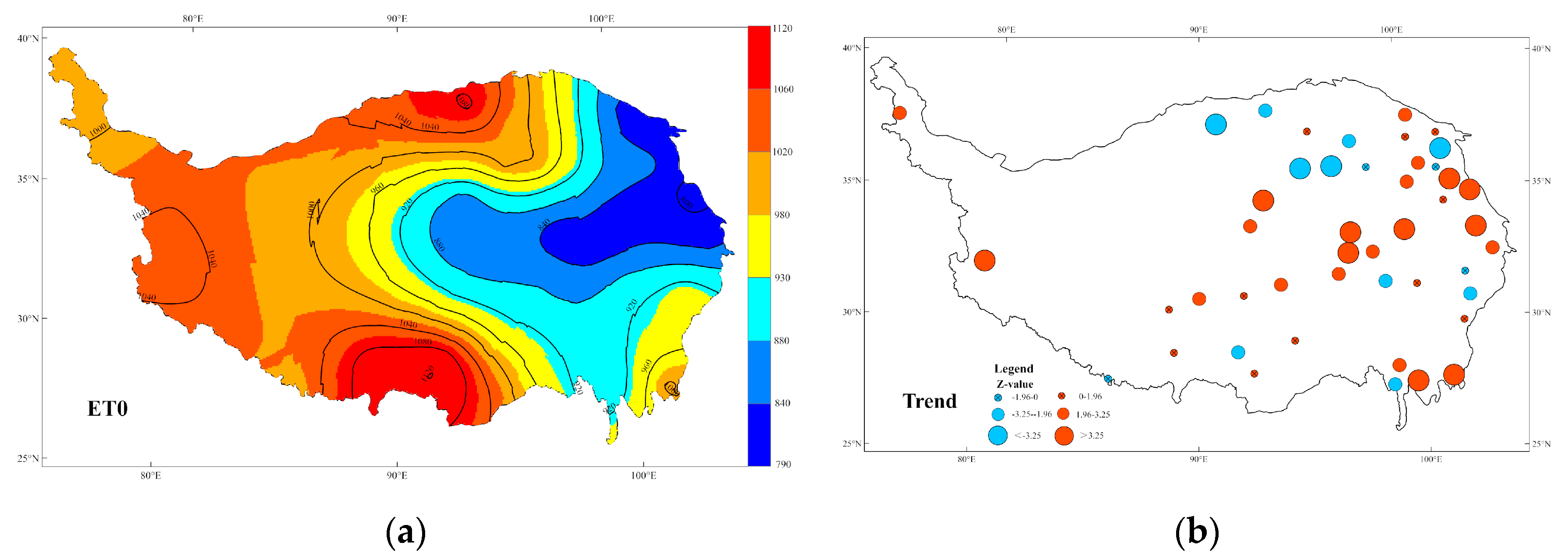
Figure 7 shows the spatial distribution trend of the annual average ET0 of the TP from 1961 to 2017 and the MK test statistical value Z of each station. Overall, the annual average ET0 of the TP gradually increased from east to west, and local peak centers appeared in the northern Qaidam Basin, the southeastern Himalayas, and the Hengduan Mountains. For the distribution of the Z values, 69.56% of the stations increased and 65.62% increased significantly, but the Qaidam Basin area decreased.
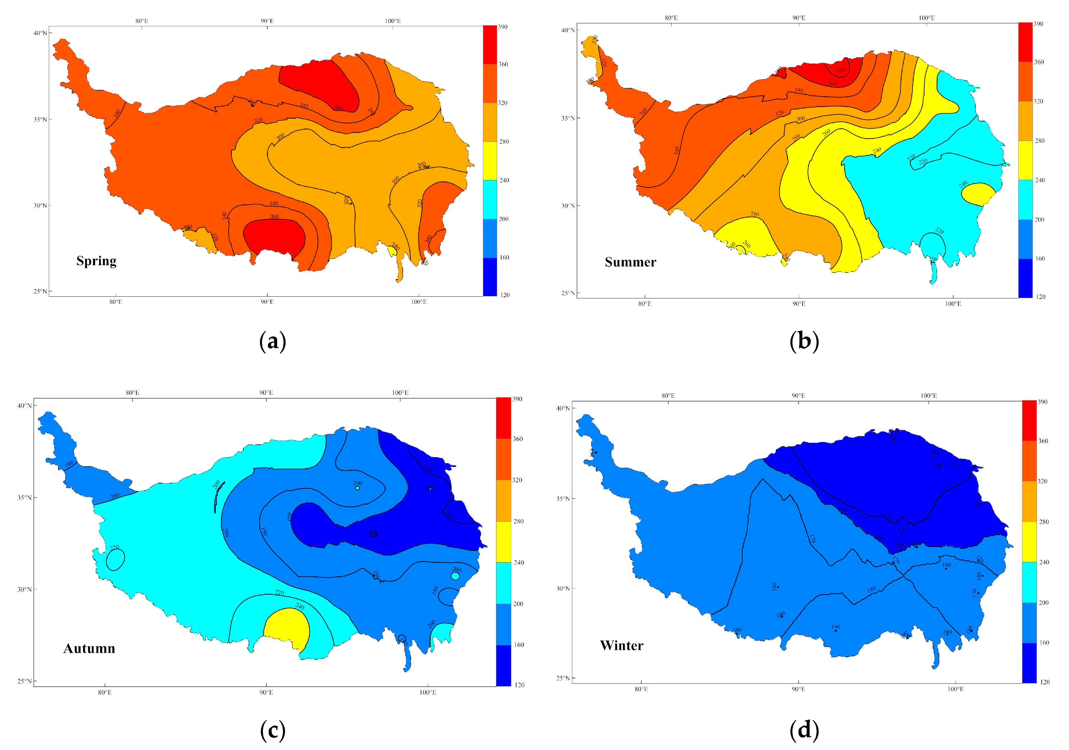
The spatial distribution of the ET0 in spring, summer, and autumn in the TP was the same as that of the annual ET0, showing an increasing trend from the east to the west (Figure 8). However, there was an increasing trend from the northeast to the southwest in winter (Figure 8d). Winter presented an increasing trend from the northeast to the southwest (Figure 8). In addition, the region had the highest average ET0 in spring and the lowest in winter. The contour of the ET0 was the densest in summer, which shows that the spatial variation is the most dramatic in this season (Figure 8b).
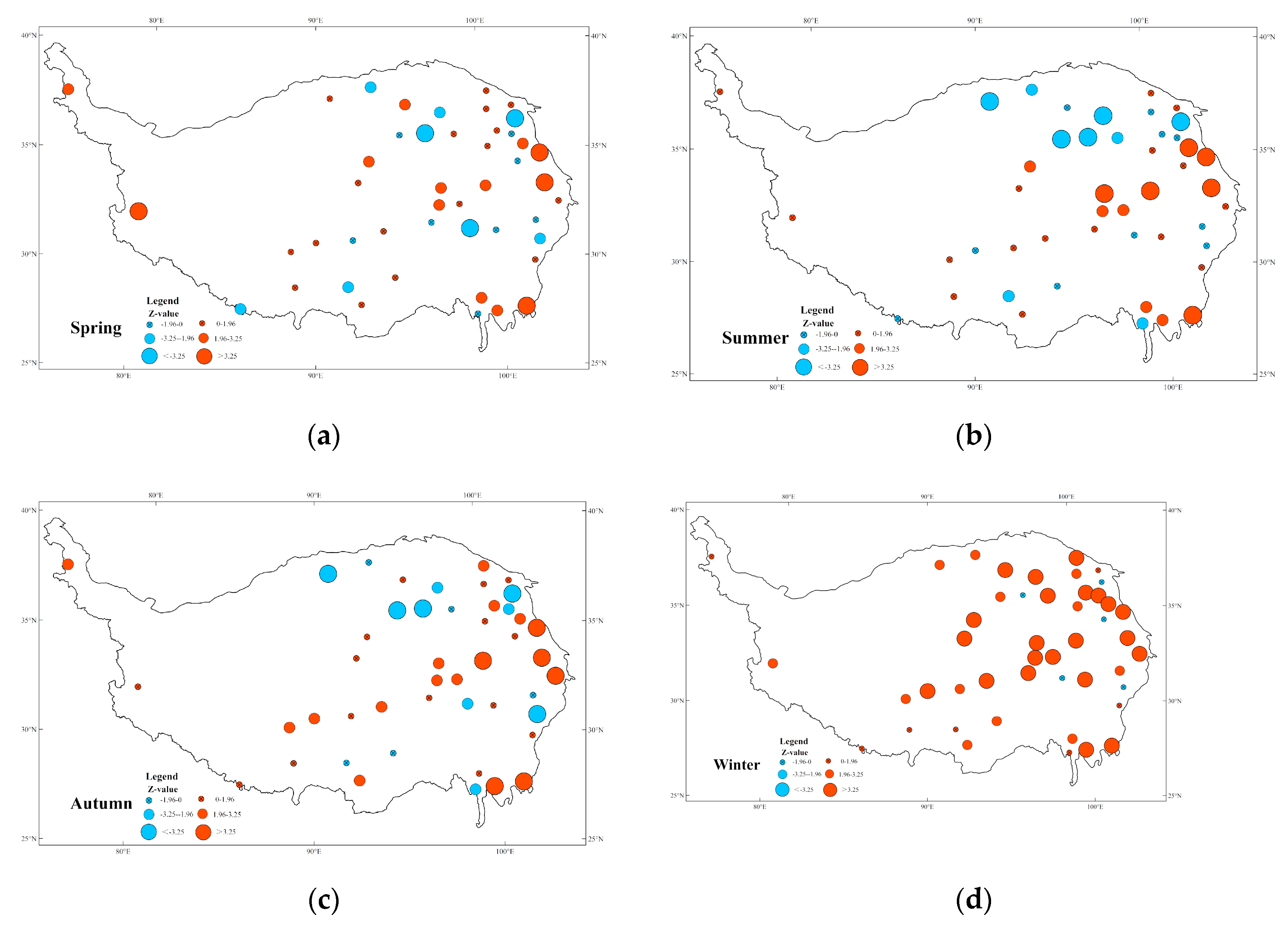
In the four seasons, the variation trend of the ET0 in spring was relatively mild, and the number of stations with a significant trend (|Z| > 1.96) accounted for only 45.65% of stations (Figure 9a), but the increasing trend of the ET0 at the two stations in the western TP was the most significant in spring. The distribution patterns in summer and autumn were similar, the decreasing trend in the Qaidam Basin was more significant in summer (Figure 9b), and the increasing trend in the TP was more obvious in autumn (Figure 9c). The increasing trend of the ET0 was the most significant in winter, with 89.13% of stations increasing, of which 73.91% increased significantly (Z > 1.96), and 26.09% of the stations increased very significantly (Z > 3.25). The number of sites showing an increasing trend gradually increased, and the increasing trend accelerated from winter to spring.

3.3. The Future Trend of ET0

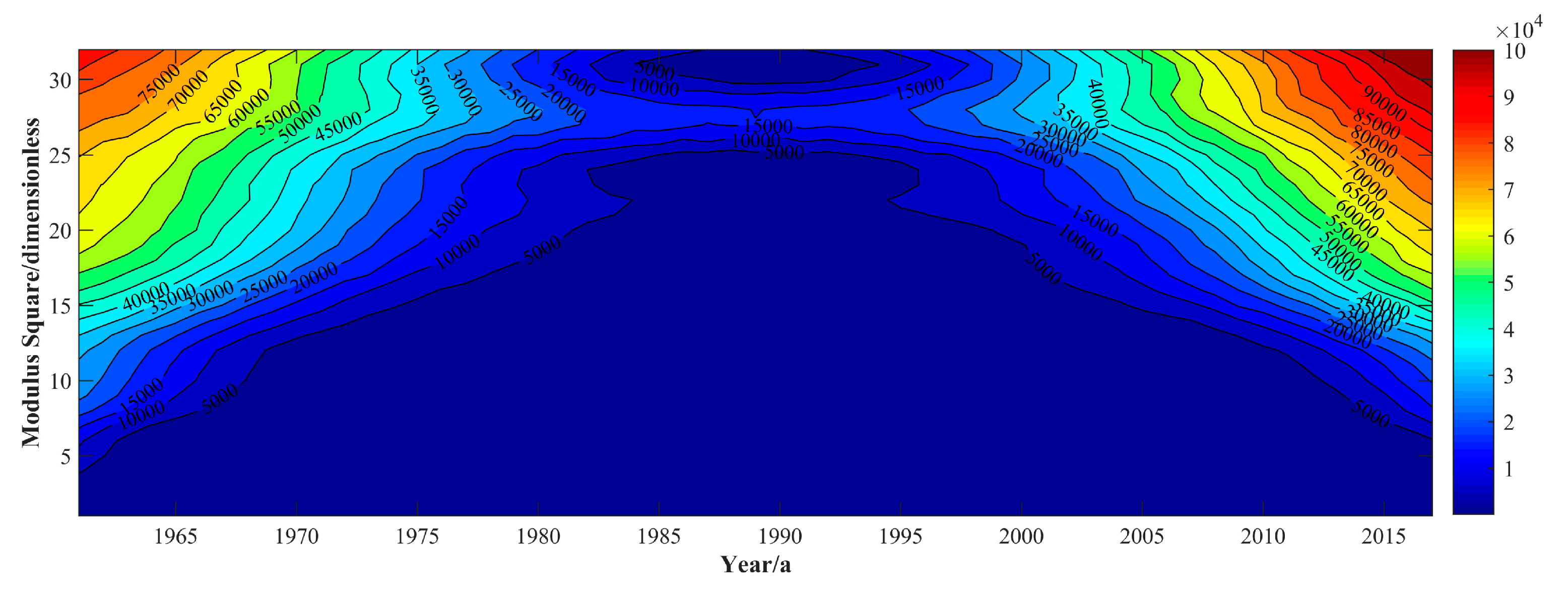
After reducing the boundary effect, the complex Morlet wavelet transformation was used to analyze the ET0 series. The isoline map of the real part of the wavelet analysis (Figure 10) and the time-frequency distribution map of the wavelet transform modulus (Figure 11) were plotted. Figure 10 shows that the 24–30a scale is very prominent, and that its scale center is approximately 27a. On this time scale, there are four partial high value centers and three low value centers in the ET0 of the TP, which occurred in 1962, 1981, 1999, and 2017 and 1973, 1989, and 2009, respectively. Figure 11 shows the oscillation energy in different periods. The oscillation energy is the strongest, and the period is the most significant, for the 20–32a time scale, but its periodic change is local (before 1973 and after 2005).
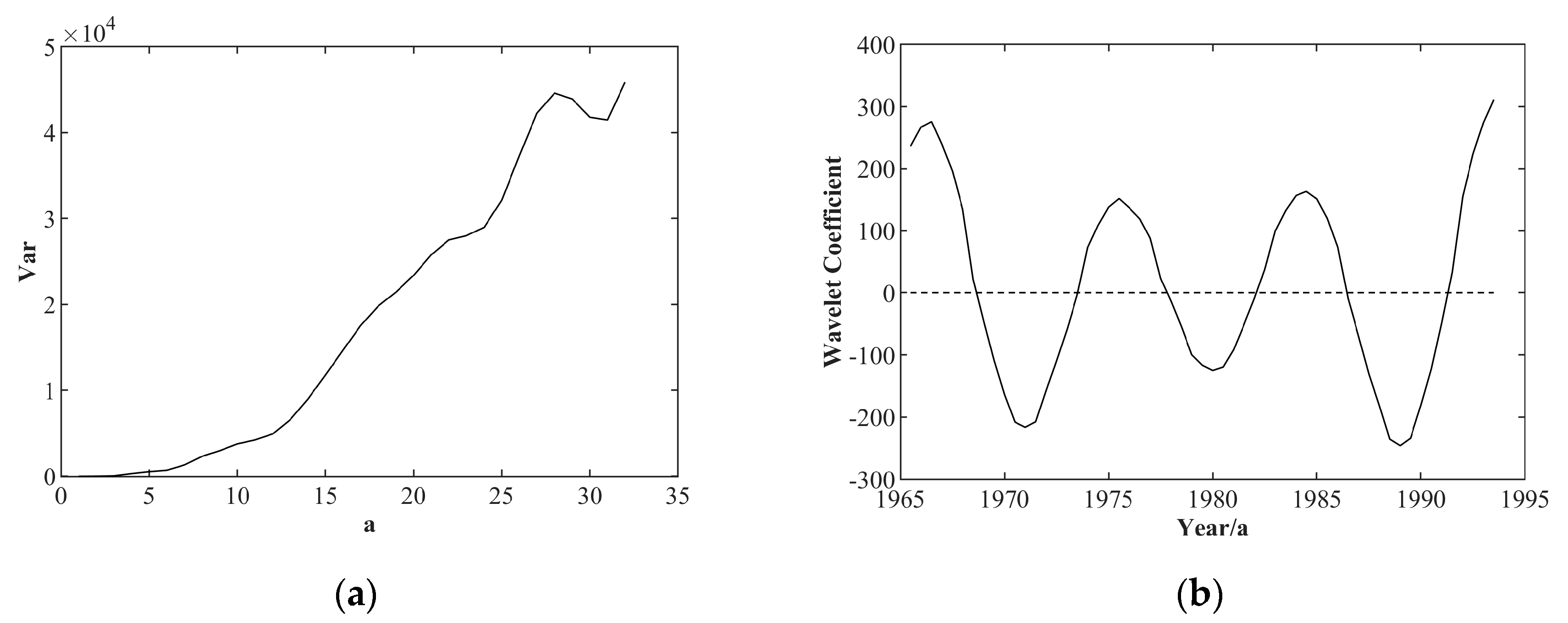
Figure 12a shows the wavelet variance diagram of the annual ET0 series over the TP. There is only one main peak value of the wavelet variance corresponding to the 28a time scale, which indicates that the ET0 sequence of the TP from 1961 to 2017 had the strongest periodic oscillation of approximately 28a, and the variance curve finally showed an upward trend, suggesting that it is likely that there will be another extreme value, indicating that there may be major periodic changes greater than 32a. Figure 12b shows that the average annual ET0 variation period of the TP is approximately 10 years on a 28a time scale, and the TP experienced approximately three wet–dry transition periods.
Table 2 shows the Hurst index of the ET0 sequence of the year and the four seasons. The Hurst index of the ET0 sequence of each time scale, calculated by the R/S analysis method, are all less than 0.5, which suggests that the future trend is anti-continuous.

3.4. The Relationships between the ET0 and Meteorological Elements and Energy Conditions

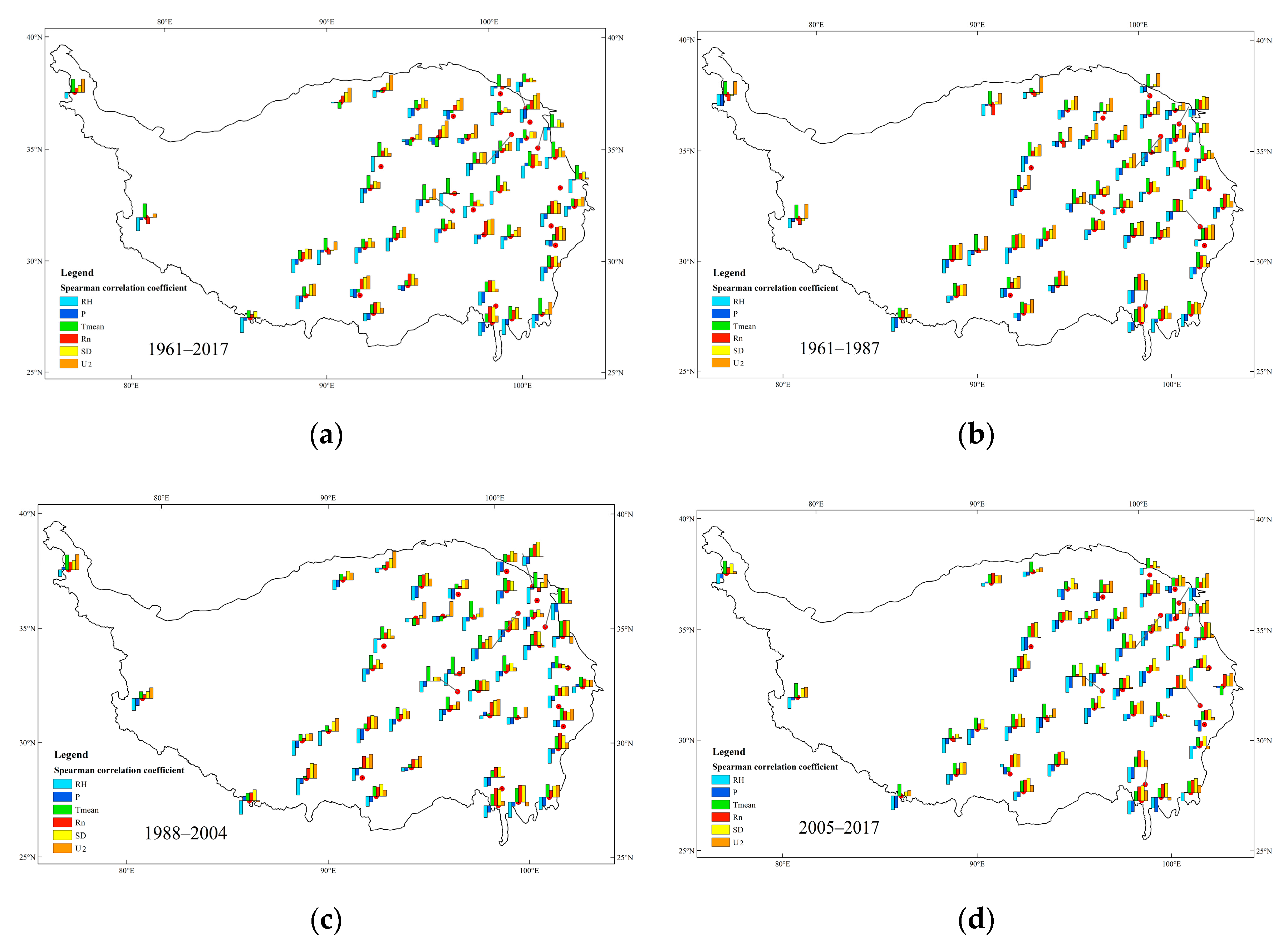
In this part, we try to explore the main factors that affect ET0 changes in different regions by comparing the correlation coefficient between the ET0 and each factor. The Spearman analysis has been used to calculate the correlations between the ET0 and RH, P, Tmean, Rn, SD, and U2 separately. Figure 13a shows the Spearman correlation coefficients between the ET0 changes of each meteorological station on the TP between 1961 and 2017 as well as other meteorological elements. There is a negative correlation between RH and P and the ET0. Tmean, Rn, SD, U2, and the ET0 in most regions were positively correlated. Among them, Tmean has had a greater impact on the central and eastern TP, Rn has had a greater impact on the central and southern regions, SD has had a greater impact on the east, and U2 has had a greater impact on the north. In addition, RH, Tmean, and U2 has had the greatest impacts on ET0.
The results in Section 3.1 show that a tendency to decrease occurred in the annual ET0 sequence of the whole region beginning in 1988, and a tendency to increase occurred beginning in 2005. The relationships between the ET0 series of these three periods and other meteorological elements were studied separately. The comparison of Figure 13b,c shows that before the first abrupt change (1961–1987), the influencing factors that had a positive correlation with the ET0 had a greater impact, especially Tmean, which had a significant impact on the entire region, and SD and U2 had a greater impact on the southern TP. After the abrupt change in 1988, the influence of RH, which had a negative correlation with the ET0, increased dramatically throughout the whole region, and the influence of Rn on the eastern region also increased. Figure 13c,d shows that after the sudden increase in 2005, the influence of RH and P on the central region increased, and the influence of U2, which has a positive correlation with the ET0, on the northeastern TP increased.

4. Discussion

4.1. Variation of ET0 Sequence

This study concludes that the ET0 of the TP showed an increasing trend between 1961 and 2017, with a particularly significant (α = 0.001) increase in ET0 occurring in winter. This is inconsistent with the phenomenon of the evaporation paradox previously discussed by many scholars. Zhang et al. and Liu et al. studied pan evaporation from the 1960s to the beginning of the 21st century and found that the TP also had an evaporation paradox [68,69]. This was caused by the inconsistent length of the time series selected in the study. The longer time series selected in this study was closer to the current changes. Similarly, the results obtained by some scholars, including those after 2005, are also find that pan evapotranspiration experienced an initial decrease, followed by an increase [70,71,72], which is consistent with those outlined here. Fan et al. also came to this conclusion that the increasing trend in the spring and winter seasons was more significant [71].

4.2. Abrupt Change in the ET0 Sequence

Similarly, the length of the time series selected also has a decisive influence on the results of change analysis. This study fully considered the limitations of the research method when conducting climate change research, and therefore, three methods, the MK test, cumulative anomaly method, and sliding t-test, were used to identify the abrupt change points. This study concludes that for the annual ET0 sequence that occurred between 1961 and 2017, there was a tendency to decrease beginning in 1988 and a tendency to increase beginning in 2005. Many scholars also concluded that abrupt changes occurred in the 1980s [45,46,51,52]. The increasing trend at the beginning of the 21st century is reported less frequently in the existing conclusions, but it was also noted by previous scholars [45]. This is because, in previous studies, the abrupt change points at the beginning of the 21st century were closer to the end of the sequence, making it impossible to draw conclusions. In this study, a time series with a length of 12 years after the abrupt change point in 2005 was detected, allowing it to be characterized as an abrupt change point. The time series selected in this paper is long enough to prove this phenomenon.

4.3. The Linkages of ET0 with Other Factors

Differing from the Pearson correlation coefficient, the Spearman correlation coefficient chosen for this study does not make assumptions about the distribution of variables and is suitable for non-parametric tests [73]. Our research found that the change in the ET0 between 1961 and 2017 had the greatest positive correlation with Tmean, followed by U2 and SD. Jian et al. similarly found an increase in the ET0, due to temperature changes [74]. Chen et al. and Xie and Zhu concurred that wind speed has an important influence on the ET0 of the TP [75,76]. Ma et al. found that energy conditions are a key factor and are also related to the SD obtained by this research [77]. Song et al. found that the decline in the ET on the TP from 2000 to 2010 could be attributed to relative humidity [78], in our research results, the ET0 also shows a strong correlation with relative humidity in this period. To further explore the differences in influencing factors in different regions, the Spearman coefficient of each site was spatially plotted. The influence on sites in high-altitude areas in southwestern China was lower for Tmean than for Rn, SD, and U2. This could be attributed to the thinner air in high-altitude areas, which is affected by energy conditions.

5. Conclusions

Based on the meteorological data measured at 46 meteorological stations on the TP between 1961 and 2017, this study calculated daily net solar radiation and ET0 using the Penman–Monteith formula. Compared with most studies, the period of this study is larger, the rules obtained are more accurate, and the research results are more convincing. In addition, to explore the time trend of ET0, the MK test, cumulative anomaly method, and sliding t-test were used to identify abrupt change points. Periodicity was explored through the Morlet wavelet analysis and Hurst index based on R/S analysis. In addition, the Spearman correlation coefficient was utilized to explore the relationship between ET0 and other meteorological elements. The main conclusions of this research are as follows:
(1)
The annual ET0 of the TP showed an increasing trend from 1961 to 2017, where the increasing trend of the ET0 in winter was particularly significant. The ET0 sequence experienced two abrupt changes. The first occurred in 1988, to initiate a decreasing trend, and the second occurred in 2005, to initiate an increasing trend.
(2)
The multiyear averaged ET0 sequence of the TP showed an increasing distribution from east to the west in space. Among the four seasons, spring showed the highest ET0, and the contours of ET0 were the densest in summer, with the most dramatic spatial changes. Three seasons, spring, summer and autumn showed a low ET0 in the east and a high ET0 in the west, but in winter, the ET0 was high in the south and low in the north.
(3)
The first main cycle of the annual ET0 in the Tibetan Plateau appeared on a 28-year time scale, and we observed three dry and wet cycles at 10-year intervals. Because the Hurst index is less than 0.5 (0.31), the future change trend of the annual ET0 series in the TP is anti-persistent.
(4)
Regarding changes in the annual ET0 sequence of the TP between 1961 and 2017, the positively correlated factor Tmean played a leading role, followed by U2 and SD, and the negatively correlated factor RH had a great impact. In addition, Rn and SD had a greater impact in high-altitude areas.

Author Contributions

Conceptualization, methodology, software, Y.L.; validation, X.Y. and Q.W.; formal analysis, writing—original draft preparation, Y.L. and Q.W.; investigation, resources, data curation, W.J. and Q.J.; supervision, project administration, funding acquisition, J.Y. All authors have participated in the review and editing. All authors have read and agreed to the published version of the manuscript.

Funding

This research was funded by the National Natural Science Foundation of China, grant number 51779007 and the National Key Research and Development Program of China, grant number 2016YFC0401308.

Acknowledgments

The authors would like to thank the China Meteorological Data Service Center (CMDC) for providing data. The authors are very grateful to the four reviewers for their professional advice, which not only improves the details and methods of this paper, but also opens up the research ideas for the next stage.

Conflicts of Interest

The authors declare no conflict of interest.

References

  1. Zylicz, T. IPCC. AURA 2015, 1, 29. [Google Scholar] [CrossRef]
  2. Seneviratne, S.I.; Corti, T.; Davin, E.L.; Hirschi, M.; Jaeger, E.B.; Lehner, I.; Orlowsky, B.; Teuling, A.J. Investigating soil moisture-climate interactions in a changing climate: A review. Earth Sci. Rev. 2010, 99, 125–161. [Google Scholar] [CrossRef]
  3. Allen, R.G.; Pereira, L.S.; Raes, D.; Smith, M. Crop Evapotranspiration: Guidelines for Computing Crop Water Requirements-FAO Irrigation and Drainage Paper 56; FAO: Rome, Italy, 1998. [Google Scholar] [CrossRef]
  4. Zhang, Y.; Chiew, F.H.S.; Peña-Arancibia, J.; Sun, F.; Li, H.; Leuning, R. Global variation of transpiration and soil evaporation and the role of their major climate drivers. J. Geophys. Res. 2017, 122, 6868–6881. [Google Scholar] [CrossRef]
  5. Gao, G.; Chen, D.; Xu, C.Y.; Simelton, E. Trend of estimated actual evapotranspiration over China during 1960–2002. J. Geophys. Res. Atmos. 2007. [Google Scholar] [CrossRef] [Green Version]
  6. Zhou, Z.; Ding, Y.; Shi, H.; Cai, H.; Fu, Q.; Liu, S.; Li, T. Analysis and prediction of vegetation dynamic changes in China: Past, present and future. Ecol. Indic. 2020, 117, 106642. [Google Scholar] [CrossRef]
  7. Sharma, V.; Nicholson, C.; Bergantino, A.; Irmak, S.; Peck, D. Temporal Trend Analysis of Meteorological Variables and Reference Evapotranspiration in the Inter-mountain Region of Wyoming. Water 2020, 12, 2159. [Google Scholar] [CrossRef]
  8. Xiang, K.; Li, Y.; Horton, R.; Feng, H. Similarity and difference of potential evapotranspiration and reference crop evapotranspiration—A review. Agric. Water Manag. 2020, 232, 106043. [Google Scholar] [CrossRef]
  9. Thornthwaite, C.W. An Approach toward a Rational Classification of Climate. Geogr. Rev. 1948, 38, 55. [Google Scholar] [CrossRef]
  10. Penman, H.L. Natural evaporation from open water, hare soil and grass. Proc. R. Soc. Lond. A Math. Phys. Sci. 1948, 193, 120–145. [Google Scholar] [CrossRef] [Green Version]
  11. Penman, H.L. Evaporation: An introductory survey. Neth. J. Agric. Sci. 1956, 4, 9–29. [Google Scholar] [CrossRef]
  12. Anonymous. Proceedings of the informal meeting on physics in agriculture. Neth. J. Agric. Sci. 1956, 4, 1–6. [Google Scholar] [CrossRef]
  13. Makkink, G.F. Testing the Penman formula by means of lysismeters. Int. Water Eng. 1957, 11, 277–288. [Google Scholar]
  14. De Vries, H. Variation in the concentration of radiocarbon with time and location on earth. Proc. K. Ned. Akad. Wet. 1958, 61, 1–9. [Google Scholar]
  15. Jensen, M. Water consumption by agricultural plants. In Water Deficits and Plant Growth: Development, Control, and Measurement; Academic Press: Cambridge, MA, USA, 1968; ISBN 0124241549. [Google Scholar]
  16. Brutsaert, W.; Parlange, M.B. Hydrologic cycle explains the evaporation paradox. Nature 1998, 396, 30. [Google Scholar] [CrossRef]
  17. Roderick, M.L.; Farquhar, G.D. The cause of decreased pan evaporation over the past 50 years. Science 2002. [Google Scholar] [CrossRef]
  18. Hobbins, M.T.; Ramírez, J.A.; Brown, T.C. Trends in pan evaporation and actual evapotranspiration across the conterminous U.S.: Paradoxical or complementary? Geophys. Res. Lett. 2004. [Google Scholar] [CrossRef] [Green Version]
  19. Jhajharia, D.; Singh, V.P.; Kumar, R.; Choudhary, R.R. Searching evidence for the existence of evaporation paradox in arid environments of northwest India. Glob. Nest J. 2014, 17, 3–11. [Google Scholar] [CrossRef] [Green Version]
  20. Rayner, D.P. Wind run changes: The dominant factor affecting pan evaporation trends in Australia. J. Clim. 2007, 20, 3379–3394. [Google Scholar] [CrossRef]
  21. Lu, X.; Bai, H.; Mu, X. Explaining the evaporation paradox in Jiangxi Province of China: Spatial distribution and temporal trends in potential evapotranspiration of Jiangxi Province from 1961 to 2013. Int. Soil Water Conserv. Res. 2016, 4, 45–51. [Google Scholar] [CrossRef] [Green Version]
  22. Huang, H.; Han, Y.; Cao, M.; Song, J.; Xiao, H.; Cheng, W. Spatiotemporal Characteristics of Evapotranspiration Paradox and Impact Factors in China in the Period of 1960–2013. Adv. Meteorol. 2015, 2015, 1–10. [Google Scholar] [CrossRef] [Green Version]
  23. Fu, G.; Charles, S.P.; Yu, J. A critical overview of pan evaporation trends over the last 50 years. Clim. Chang. 2009, 97, 193–214. [Google Scholar] [CrossRef]
  24. Zhang, Q.; Wang, W.; Wang, S.; Zhang, L. Increasing trend of pan evaporation over the semiarid loess plateau under a warming climate. J. Appl. Meteorol. Climatol. 2016, 55, 2007–2020. [Google Scholar] [CrossRef]
  25. Huang, X.; Ma, L.; Liu, T.; Sun, B.; Zhou, Y.; Yang, C.; Qiao, Z. Spatial and temporal variability of the abrupt interannual temperature change and warming hiatus in China, 1951–2016. Meteorol. Appl. 2020. [Google Scholar] [CrossRef]
  26. Shi, P.J.; Sun, S.; Wang, M.; Li, N.; Wang, J.A.; Jin, Y.Y.; Gu, X.T.; Yin, W.X. Climate change regionalization in China (1961–2010). Sci. China Earth Sci. 2014. [Google Scholar] [CrossRef]
  27. Wu, H.; Hou, W.; Qian, Z.H.; Hu, J.G. The research on the sensitivity of climate change in China in recent 50 years based on composite index. Wuli Xuebao Acta Phys. Sin. 2012. [Google Scholar] [CrossRef]
  28. Wang, B.; Hong, G.; Cui, C.-Q.; Yu, H.; Murty, T. Comprehensive analysis on China’s National Climate Change Assessment Reports: Action and emphasis. Front. Eng. Manag. 2019, 6, 52–61. [Google Scholar] [CrossRef]
  29. Immerzeel, W.W.; Droogers, P.; de Jong, S.M.; Bierkens, M.F.P. Large-scale monitoring of snow cover and runoff simulation in Himalayan river basins using remote sensing. Remote Sens. Environ. 2009, 113, 40–49. [Google Scholar] [CrossRef]
  30. Deng, C.; Zhang, W. Spatiotemporal distribution and the characteristics of the air temperature of a river source region of the Qinghai-Tibet Plateau. Environ. Monit. Assess. 2018, 190, 368. [Google Scholar] [CrossRef]
  31. Liu, Z.; Yao, Z.; Wang, R.; Yu, G. Estimation of the Qinghai-Tibetan Plateau runoff and its contribution to large Asian rivers. Sci. Total Environ. 2020, 749, 141570. [Google Scholar] [CrossRef]
  32. Zhou, D.; Hao, L.; Kim, J.B.; Liu, P.; Pan, C.; Liu, Y.; Sun, G. Potential impacts of climate change on vegetation dynamics and ecosystem function in a mountain watershed on the Qinghai-Tibet Plateau. Clim. Chang. 2019, 156, 31–50. [Google Scholar] [CrossRef]
  33. Cao, S.; Cao, G.; Han, G.; Wu, F.; Lan, Y. Comparison of evapotranspiration between two alpine type wetland ecosystems in Qinghai lake basin of Qinghai-Tibet Plateau. Ecohydrol. Hydrobiol. 2020, 20, 215–229. [Google Scholar] [CrossRef]
  34. Guo, B.; Zang, W.; Yang, F.; Han, B.; Chen, S.; Liu, Y.; Yang, X.; He, T.; Chen, X.; Liu, C.; et al. Spatial and temporal change patterns of net primary productivity and its response to climate change in the Qinghai-Tibet Plateau of China from 2000 to 2015. J. Arid Land 2020. [Google Scholar] [CrossRef] [Green Version]
  35. Zhang, G.; Chen, F.; Chen, Y.; Li, J.; Peng, X. Evaluation of Noah-MP land-model uncertainties over sparsely vegetated sites on the Tibet Plateau. Atmosphere 2020, 11, 458. [Google Scholar] [CrossRef]
  36. Yin, Y.; Han, C.; Yang, G.; Huang, Y.; Liu, M.; Wang, X. Changes in the summer extreme precipitation in the Jianghuai plum rain area and their relationship with the intensity anomalies of the south Asian high. Atmos. Res. 2020, 236, 104793. [Google Scholar] [CrossRef]
  37. Guo, X.; Yang, Y.; Li, Z.; You, L.; Zeng, C.; Cao, J.; Hong, Y. Drought trend analysis based on the standardized precipitation-evapotranspiration index using NASA’s earth exchange global daily downscaled projections, high spatial resolution coupled model intercomparison project phase 5 projections, and assessment of p. Water 2019, 11, 2455. [Google Scholar] [CrossRef] [Green Version]
  38. Ye, C.; Sun, J.; Liu, M.; Xiong, J.; Zong, N.; Hu, J.; Huang, Y.; Duan, X.; Tsunekawa, A. Concurrent and Lagged Effects of Extreme Drought Induce Net Reduction in Vegetation Carbon Uptake on Tibetan Plateau. Remote Sens. 2020, 12, 2347. [Google Scholar] [CrossRef]
  39. Wang, P.; Wu, X.; Hao, Y.; Wu, C.; Zhang, J. Is Southwest China drying or wetting? Spatiotemporal patterns and potential causes. Theor. Appl. Climatol. 2020, 139, 1–15. [Google Scholar] [CrossRef]
  40. Zhang, H.; Ding, M.; Li, L.; Liu, L. Continuous Wetting on the Tibetan Plateau during 1970–2017. Water 2019, 11, 2605. [Google Scholar] [CrossRef] [Green Version]
  41. Lu, Y.; Jiang, S.; Ren, L.; Zhang, L.; Wang, M.; Liu, R.; Wei, L. Spatial and Temporal variability in precipitation concentration over mainland China, 1961–2017. Water 2019, 11, 881. [Google Scholar] [CrossRef] [Green Version]
  42. Tao, Y.; Wang, W.; Song, S.; Ma, J. Spatial and temporal variations of precipitation extremes and seasonality over China from 1961–2013. Water 2018, 10, 719. [Google Scholar] [CrossRef] [Green Version]
  43. Hu, Y.; Xu, J.; Huang, Y.; Zhou, Y.; Pang, Y.; Shi, Z.; Chen, X. Spatial and temporal variations in the rainy season onset over the Qinghai-Tibet Plateau. Water 2019, 11, 1960. [Google Scholar] [CrossRef] [Green Version]
  44. Sun, S.; Chen, B.; Shao, Q.; Chen, J.; Liu, J.; Zhang, X.J.; Zhang, H.; Lin, X. Modeling evapotranspiration over China’s landmass from 1979 to 2012 using multiple land surface models: Evaluations and analyses. J. Hydrometeorol. 2017, 18, 1185–1203. [Google Scholar] [CrossRef]
  45. Yao, T.; Lu, H.; Feng, W.; Yu, Q. Evaporation abrupt changes in the Qinghai-Tibet Plateau during the last half-century. Sci. Rep. 2019, 9. [Google Scholar] [CrossRef] [PubMed]
  46. Wang, W.; Xing, W.; Shao, Q.; Yu, Z.; Peng, S.; Yang, T.; Yong, B.; Taylor, J.; Singh, V.P. Changes in reference evapotranspiration across the Tibetan Plateau: Observations and future projections based on statistical downscaling. J. Geophys. Res. Atmos. 2013, 118, 4049–4068. [Google Scholar] [CrossRef]
  47. Jiang, C.; Li, D.; Gao, Y.; Liu, W.; Zhang, L. Impact of climate variability and anthropogenic activity on streamflow in the Three Rivers Headwater Region, Tibetan Plateau, China. Theor. Appl. Climatol. 2017, 129, 667–681. [Google Scholar] [CrossRef]
  48. Attarod, P.; Miri, S.; Shirvany, A.; Bayramzadeh, V. Variations in leaf area index of Quercus brantii trees in response to changing climate. J. Agric. Sci. Technol. 2018, 20, 1417–1429. [Google Scholar]
  49. Sönmez, A.Y.; Kale, S. Climate change effects on annual streamflow of filyos river (Turkey). J. Water Clim. Chang. 2018, 11, 420–433. [Google Scholar] [CrossRef]
  50. Chu, R.; Li, M.; Islam, A.R.M.T.; Fei, D.; Shen, S. Attribution analysis of actual and potential evapotranspiration changes based on the complementary relationship theory in the Huai River basin of eastern China. Int. J. Climatol. 2019, 39, 4072–4090. [Google Scholar] [CrossRef]
  51. Wang, J.; Gao, Y.; Wang, S. Assessing the response of runoff to climate change and human activities for a typical basin in the Northern Taihang Mountain, China. J. Earth Syst. Sci. 2018, 127, 37. [Google Scholar] [CrossRef] [Green Version]
  52. Liu, R.; Wen, J.; Wang, X.; Wang, Z. Validation of evapotranspiration and its long-term trends in the yellow river source region. J. Water Clim. Chang. 2017, 8, 495–509. [Google Scholar] [CrossRef]
  53. Sharma, C.; Ojha, C.S.P. Modified Signal-to-Noise Ratio Method for Early Detection of Climate Change. J. Hydrol. Eng. 2020, 25, 04020032. [Google Scholar] [CrossRef]
  54. Liu, X.; Yang, W.; Zhao, H.; Wang, Y.; Wang, G. Effects of the freeze-thaw cycle on potential evapotranspiration in the permafrost regions of the Qinghai-Tibet Plateau, China. Sci. Total Environ. 2019, 687, 257–266. [Google Scholar] [CrossRef] [PubMed]
  55. Tapponnier, P.; Zhiqin, X.; Roger, F.; Meyer, B.; Arnaud, N.; Wittlinger, G.; Jingsui, Y. Oblique stepwise rise and growth of the tibet plateau. Science 2001, 294, 1671–1677. [Google Scholar] [CrossRef] [PubMed]
  56. Qiu, J. China: The third pole. Nature 2008, 454, 393–396. [Google Scholar] [CrossRef] [Green Version]
  57. Chen, H.; Zhu, Q.; Peng, C.; Wu, N.; Wang, Y.; Fang, X.; Gao, Y.; Zhu, D.; Yang, G.; Tian, J.; et al. The impacts of climate change and human activities on biogeochemical cycles on the Qinghai-Tibetan Plateau. Glob. Chang. Biol. 2013, 19, 2940–2955. [Google Scholar] [CrossRef]
  58. Luo, W.; Zhang, G.; Chen, W.; Xu, F. Response of glacial lakes to glacier and climate changes in the western Nyainqentanglha range. Sci. Total Environ. 2020, 735, 139607. [Google Scholar] [CrossRef]
  59. Yu, G.A.; Lu, J.; Lyu, L.; Han, L.; Wang, Z. Mass flows and river response in rapid uplifting regions—A case of lower Yarlung Tsangpo basin, southeast Tibet, China. Int. J. Sediment Res. 2020. [Google Scholar] [CrossRef]
  60. Han, J.; Wang, J.; Zhao, Y.; Wang, Q.; Zhang, B.; Li, H.; Zhai, J. Spatio-temporal variation of potential evapotranspiration and climatic drivers in the Jing-Jin-Ji region, North China. Agric. For. Meteorol. 2018, 75–83. [Google Scholar] [CrossRef]
  61. Ye, J.; Guo, A.; Sun, G. Statistical analysis of reference evapotranspiration on the tibetan Plateau. J. Irrig. Drain. Eng. 2009. [Google Scholar] [CrossRef]
  62. Bhardwaj, A.; Misra, V. Defining the Northeast Monsoon of India. Mon. Weather Rev. 2019, 147, 791–807. [Google Scholar]
  63. Peng, D.; Qiu, L.; Fang, J.; Zhang, Z. Quantification of Climate Changes and Human Activities That Impact Runoff in the Taihu Lake Basin, China. Math. Probl. Eng. 2016, 2016. [Google Scholar] [CrossRef] [Green Version]
  64. Hůnová, I.; Bäumelt, V.; Modlík, M. Long-term trends in nitrogen oxides at different types of monitoring stations in the Czech Republic. Sci. Total Environ. 2019, 699, 134378. [Google Scholar] [CrossRef] [PubMed]
  65. Gocic, M.; Trajkovic, S. Analysis of changes in meteorological variables using Mann-Kendall and Sen’s slope estimator statistical tests in Serbia. Glob. Planet. Chang. 2013, 100, 172–182. [Google Scholar] [CrossRef]
  66. Sun, J.; Wang, X.; Shahid, S. Precipitation and runoff variation characteristics in typical regions of North China Plain: A case study of Hengshui City. Theor. Appl. Climatol. 2020, 1–15. [Google Scholar] [CrossRef]
  67. Kumar, N.; Tischbein, B.; Beg, M.K. Multiple trend analysis of rainfall and temperature for a monsoon-dominated catchment in India. Meteorol. Atmos. Phys. 2018, 131, 1019–1033. [Google Scholar] [CrossRef]
  68. Zhang, Y.; Liu, C.; Tang, Y.; Yang, Y. Trends in pan evaporation and reference and actual evapotranspiration across the Tibetan Plateau. J. Geophys. Res. Atmos. 2007. [Google Scholar] [CrossRef]
  69. Liu, X.; Zheng, H.; Zhang, M.; Liu, C. Identification of dominant climate factor for pan evaporation trend in the Tibetan Plateau. J. Geogr. Sci. 2011, 21, 594–608. [Google Scholar] [CrossRef]
  70. Cong, Z.T.; Yang, D.W.; Ni, G.H. Does evaporation paradox exist in China? Hydrol. Earth Syst. Sci. 2009, 13, 357–366. [Google Scholar] [CrossRef] [Green Version]
  71. Fan, J.; Wu, L.; Zhang, F.; Xiang, Y.; Zheng, J. Climate change effects on reference crop evapotranspiration across different climatic zones of China during 1956–2015. J. Hydrol. 2016, 542, 923–937. [Google Scholar] [CrossRef]
  72. Liu, X.; Luo, Y.; Zhang, D.; Zhang, M.; Liu, C. Recent changes in pan-evaporation dynamics in China. Geophys. Res. Lett. 2011. [Google Scholar] [CrossRef] [Green Version]
  73. Patakamuri, S.K.; Muthiah, K.; Sridhar, V. Long-Term homogeneity, trend, and change-point analysis of rainfall in the arid district of ananthapuramu, Andhra Pradesh State, India. Water 2020, 12, 211. [Google Scholar] [CrossRef] [Green Version]
  74. Jian, D.; Ma, Z.; Chen, L.; Duan, J.; Mitchell, D.; Zheng, Z.; Lv, M.; Zhang, H. Effects of 1.5 °C and 2 °C of warming on regional reference evapotranspiration and drying: A case study of the Yellow River Basin, China. Int. J. Climatol. 2020. [Google Scholar] [CrossRef]
  75. Xie, H.; Zhu, X. Reference evapotranspiration trends and their sensitivity to climatic change on the Tibetan Plateau (1970–2009). Hydrol. Process. 2012, 27, 3685–3693. [Google Scholar] [CrossRef]
  76. Shenbin, C.; Yunfeng, L.; Thomas, A. Climatic change on the Tibetan Plateau: Potential evapotranspiration trends from 1961-2000. Clim. Chang. 2006, 76, 291–319. [Google Scholar] [CrossRef]
  77. Ma, Y.J.; Li, X.Y.; Liu, L.; Yang, X.F.; Wu, X.C.; Wang, P.; Lin, H.; Zhang, G.H.; Miao, C.Y. Evapotranspiration and its dominant controls along an elevation gradient in the Qinghai Lake watershed, northeast Qinghai-Tibet Plateau. J. Hydrol. 2019, 575, 257–268. [Google Scholar] [CrossRef]
  78. Song, L.; Zhuang, Q.; Yin, Y.; Zhu, X.; Wu, S. Spatio-temporal dynamics of evapotranspiration on the Tibetan Plateau from 2000 to 2010. Environ. Res. Lett. 2017, 12, 014011. [Google Scholar] [CrossRef]
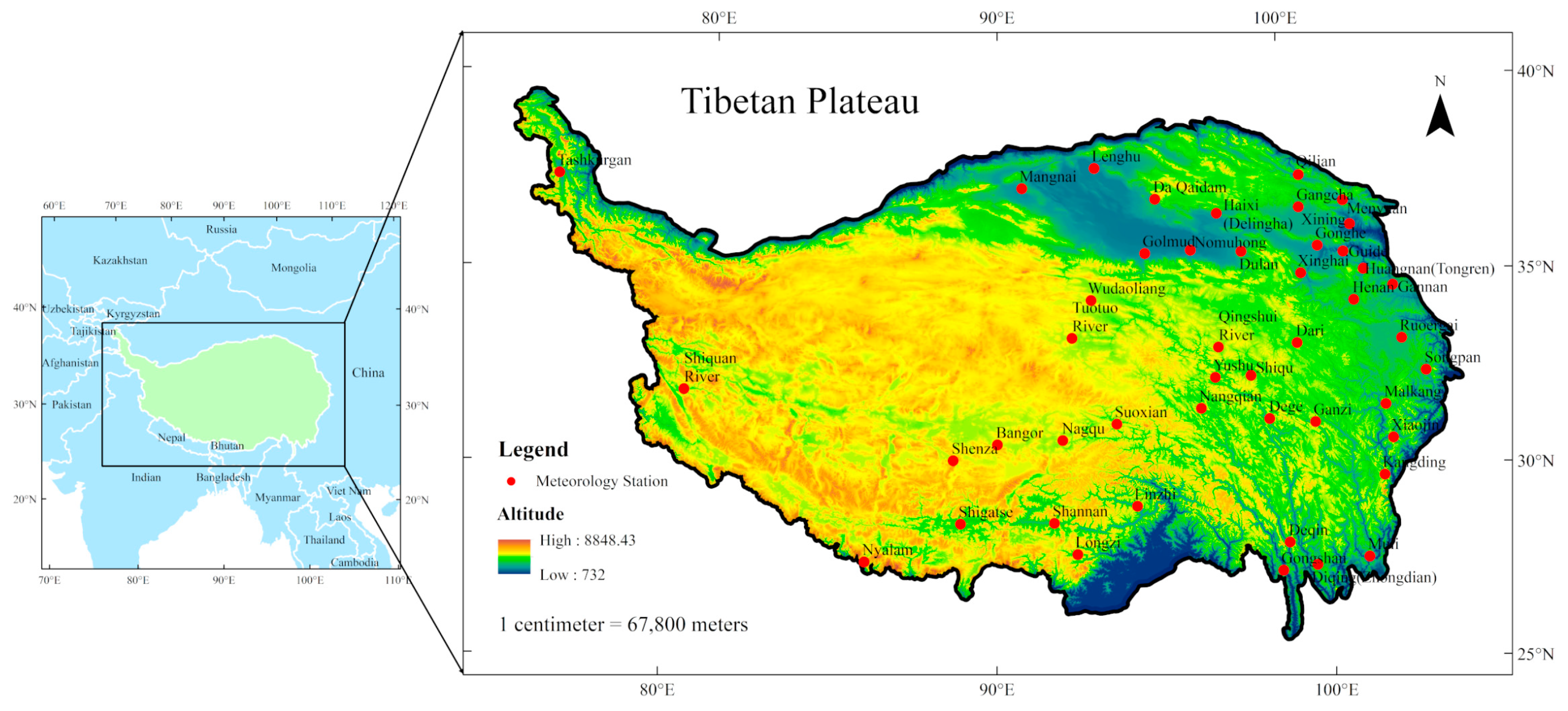
Figure 1. The location of the Qinghai-Tibet Plateau and the distribution of meteorological stations.
Water 12 03178 g001
Figure 2. The abrupt change point identification diagram of the reference evapotranspiration (ET0) sequence, where (a) is the cumulative anomaly curve; (b) is the positive and negative sequence line of the Mann–Kendall (MK) test; and (c) is the sliding t-test curve with three steps, and the corresponding color is marked as the peak value of each curve.
Water 12 03178 g002
Figure 3. The abrupt change point identification diagram of spring ET0 sequence, where the picture category of the (ac) is same to Figure 2.
Water 12 03178 g003
Figure 4. The abrupt change point identification diagram of summer ET0 sequence, where the picture category of the (ac) is same to Figure 2.
Water 12 03178 g004
Figure 5. The abrupt change point identification diagram of autumn ET0 sequence, where the picture category of the (ac) is same to Figure 2.
Water 12 03178 g005
Figure 6. The abrupt change point identification diagram of winter ET0 sequence, where the picture category of the (ac) is same to Figure 2.
Water 12 03178 g006
Figure 7. (a) The distribution of the multi-year average ET0 in the Tibetan Plateau (TP); (b) the distribution of the statistical value Z of the Mann–Kendall test at each station of TP from 1961 to 2017. At the α = 0.05 significance level, if |Z| > 1.96, ET0 changes significantly. The red bubble represents the increasing trend, the blue bubble represents the decreasing trend, and a larger bubble size suggests an increased significance.
Water 12 03178 g007
Figure 8. The spatial distribution of ET0 in the four seasons, where (a) is spring; (b) is summer; (c) is autumn; (d) is winter.
Water 12 03178 g008
Figure 9. The distribution of the of the Mann–Kendall Z statistic for ET0 series at each station of from 1961 to 2017, where (a) is spring; (b) is summer; (c) is autumn; (d) is winter. The significance level and expression method are the same as in Figure 7b.
Water 12 03178 g009
Figure 10. Contour map of the real part of wavelet coefficients.
Water 12 03178 g010
Figure 11. Time-frequency distribution of the wavelet transform modulus.
Water 12 03178 g011
Figure 12. (a) The wavelet variance analysis chart; (b) the wavelet coefficient chart for the 28a time scale.
Water 12 03178 g012
Figure 13. Distribution of correlation between the ET0 and other factors; (a) 1961–2017, (b) before the first abrupt change (1961–1987); (c) between two abrupt changes (1988–2004); (d) after the second abrupt change (2005–2017).
Water 12 03178 g013
Table 1. Z-values from the Mann–Kendall (MK) test of reference evapotranspiration (ET0) at different scales.
ScaleYearSpringSummerAutumnWinter
Z value1.591.58−1.080.863.93 ***
*** Significance level of 0.001 (p < 0.001).
Table 2. The Hurst index of the ET0 series for the year and four seasons.
ScaleYearSpringSummerAutumnWinter
Hurst index0.310.210.280.300.31
Publisher’s Note: MDPI stays neutral with regard to jurisdictional claims in published maps and institutional affiliations.