Investigating River Water/Groundwater Interaction along a Rivulet Section by ²²²Rn Mass Balancing

Abstract

Investigation of river water/groundwater interaction aims generally at: (i) localizing water migration pathways; and (ii) quantifying water and associated matter exchange between the two natural water resources. Related numerical models generally rely on model-specific parameters that represent the physical conditions of the catchment and suitable aqueous tracer data. A generally applicable approach for this purpose is based on the finite element model FINIFLUX that is using the radioactive noble gas radon-222 as naturally occurring tracer. During the study discussed in this paper, radon and physical stream data were used with the aim to localize and quantify groundwater discharge into a well-defined section of a small headwater stream. Besides site-specific results of two sampling campaigns, the outcomes of the study reveal: (i) the general difficulties of conducting river water/groundwater interaction studies in small and heterogeneous headwater catchments; and (ii) the particular challenge of defining well constrained site- and campaign-specific values for both the groundwater radon endmember and the radon degassing coefficient. It was revealed that determination of both parameters should be based on as many data sources as possible and include a critical assessment of the reasonability of the gathered and used datasets. The results of our study exposed potential limitations of the approach if executed in small and turbulent headwater streams. Hence, we want to emphasize that the project was not only executed as a case study at a distinct site but rather aimed at evaluating the applicability of the chosen approach for conducting river water/groundwater interaction studies in heterogeneous headwater catchments.

1. Introduction

Groundwater and surface water differ generally in their chemical, physical and biological properties. Thus, water exchange between these two hydrological domains affects the water quality of both types of water bodies. In addition to the physical water exchange, various biogeochemical processes occur at the groundwater–surface water interface (i.e., in the hyporheic zone), resulting in retention, transformation, precipitation and/or sorption of chemical substances (e.g., [1]). Hence, localizing pathways as well as quantifying both physical water exchange and the associated matter flux is crucial for the understanding and protection of natural water resources and, if required, for the design and implementation of remediation strategies.

The interaction between groundwater and surface water can be directed in two ways: (i) groundwater discharging into the surface water body; and (ii) surface water infiltrating into the aquifer. In the case of watercourses, we distinguish accordingly between gaining sections (with groundwater discharging through the hyporheic zone into the stream) and losing sections (with stream water infiltrating through the hyporheic zone into the aquifer). Depending on the physical gradient between the stream water level and the hydraulic head of the surrounding aquifer, gaining and losing sections can alternate not only with time (i.e., seasonally or on short-term, e.g., during storm events) but also in space, even over short distances. For instance, a decrease in the groundwater discharge rate or even a change from gaining to losing may be triggered by a pressure increase on the streambed caused by a temporarily rising river water level due to a flood event (e.g., [2]) or due to a temporary obstacle on the streambed (e.g., [3]). A review of the principal drivers and mechanisms of groundwater/surface water exchange was published by Sophocleous [4]. Kalbus et al. [5] discussed a range of available methodical approaches for its investigation.

Numerical modeling is an essential tool for the investigation of groundwater/surface water exchange and for the evaluation of the associated matter fluxes. The models rely on model-specific parameters and indicators that represent case-specific physical conditions of the catchment. Environmental tracers (i.e., naturally occurring substances that show a significant concentration gradient between hydraulically connected groundwater and surface water domains) have proven suitable tools to disentangle water flow pathways and to parameterize numerical models in order to derive site-specific water and solute fluxes.

In this study, we demonstrated the use of the ubiquitously occurring radioactive noble gas radon (²²²Rn) as an environmental tracer for localizing and quantifying water fluxes from groundwater into stream reaches that are subject to alternating water gaining and losing conditions. The study was carried out along a defined and well-studied 1050 m reach of a rivulet in the Harz Mountains, Germany (cf. Figure 1). A rivulet was purposely chosen as study site because the major part of any catchment’s overall groundwater discharge is entering the surface water in the network of headwater rivulets, making the hyporheic zone of these rivulets the dominant domain for biogeochemical processes [6]. However, while radon has been used to map and quantify groundwater discharge to larger rivers already in the past (predominantly gaining rivers with >1 m³ s⁻¹ river discharge; e.g., [7,8,9]), the approach has rarely been used for studying small headwaters with more rapidly changing hydrological boundary conditions and alternating gaining and losing sections. Hence, besides producing site-specific results, a general aim of the study was evaluating the applicability of the approach for small headwater streams.

For numerical mass-balance modeling of radon, we applied the implicit finite element model FINIFLUX [10]. All input parameters required for the model were measured during two sampling campaigns that reflected strongly contrasting hydraulic conditions within the catchment. During the two campaigns, we measured the radon concentrations of both the rivulet water and the hydraulically connected groundwater directly on site by means of mobile radon detection equipment. Since the loss of radon by degassing plays a significant role in shallow and turbulent watercourses, the radon degassing coefficient (k) was determined based on four different approaches that use either empirical equations (two approaches) or direct measurements in the field (two approaches). This application of several individual approaches for radon degassing evaluation allowed (besides a better assessment of the respective site-specific results) their comparison, i.e., a general evaluation of their advantages and disadvantage if used for studies in small headwater rivulets. For direct measurement of k in the field, two indicators were chosen: the radon concentration decrease in losing subsections of the rivulet (Field Campaign 1) and the concentration decrease of propane downstream of a propane point injection (Field Campaign 2). The two empirical approaches are discussed in Section 2.2.2. Furthermore, the rivulet discharge rate was determined using salt pulse tracer injections and continuous bromide injections. Water conductivity and temperature were recorded by means of mobile sensors.

2. Materials and Methods

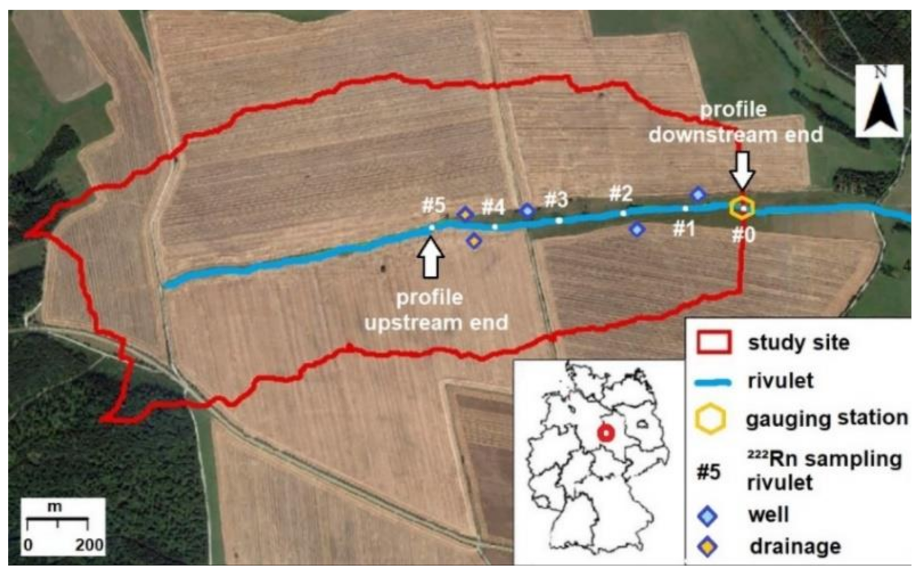
2.1. Study Area

The study was executed within the research catchment “Schaefertal”, which is part of a first-order catchment located in the Harz Mountains, Central Germany. The Schaefertal rivulet runs through the catchment’s central axis from west to east. The studied section of the rivulet reaches from a gauging station at the catchment outlet (downstream end of the investigated profile) to 1050 m upstream (Figure 1). The “Schaefertal” research site spreads from the uppermost western part of the catchment down to the gauging station and covers an area of 1.44 km². The gauging station is the only pathway for water discharge out of the research site because of a 55 m long and 7 m deep subsurface barrier that blocks all subsurface flow out of it. The site has been subject to hydrological research since 1968 (e.g., [11]).

Surface elevations within the site range from a maximum of 473 masl in the west to 393 masl at the gauging station in the east. Within the central axis (i.e., the riparian zone of the Schaefertal rivulet), the soils are dominated by Gleysols and Luvisols. The surrounding hillslopes are dominated by Luvisols and Cambisols and are mainly used for agriculture [12]. Two small stands of forest are located near the western, i.e., uphill edge of the catchment.

The local aquifer consists of two major domains: (i) an upper ca. 0.5 m layer with rather high permeability and a well-developed root zone; and (ii) a subjacent layer with a high loam content and thus lower permeability [13]. The overall aquifer thickness varies from 2 m at the top of the slopes to 5 m at the valley bottom with a 2.4 m average [12].

Two sampling campaigns were carried out during the study. Although both campaigns were carried out during the winter with low air and water temperatures, they reflect strongly differing hydrological conditions (see Supplementary Materials: “Water level, Q, prec.”). During the first campaign (22 January 2019), the catchment was partly covered with snow, outside temperatures were well below 0 °C and groundwater recharge was low during the previous weeks. That resulted in a low rivulet discharge rate of only about 6 L s⁻¹ measured at the gauging station. Thus, the first campaign is referred to as “low-flow campaign” in the following.

During the second campaign three weeks later (13 February 2019), the catchment soils were saturated with water due to recent snowmelt in addition to considerable rains during the five days preceding the campaign (in total ca. 31 mm). Outside temperatures were around 5 °C and rivulet discharge was more than seven times as high as during the first campaign (about 45 L s⁻¹ at the gauging station). Thus, the second campaign is referred to as “high-flow campaign” in the following.

2.2. Onsite Methods

2.2.1. Radon as Aqueous Tracer

Radon (²²²Rn) is constantly produced in every aquifer matrix by radioactive decay of its parent nuclide ²²⁶Ra. In contrast, its production in surface water bodies is generally negligible. Consequently, radon activity concentrations in groundwater are in general about 3–5 orders of magnitude higher than in surface waters.

If groundwater discharges into a surface water body, the groundwater derived radon is lost quickly due to both degassing to the atmosphere and radioactive decay (half-life 3.8 days). That allows: (i) using radon distribution patterns along a watercourse for the localization of groundwater discharge zones; and (ii) using radon mass balances within a defined sub-reach of the watercourse for the quantification of groundwater discharge and thus for the investigation of the associated matter fluxes.

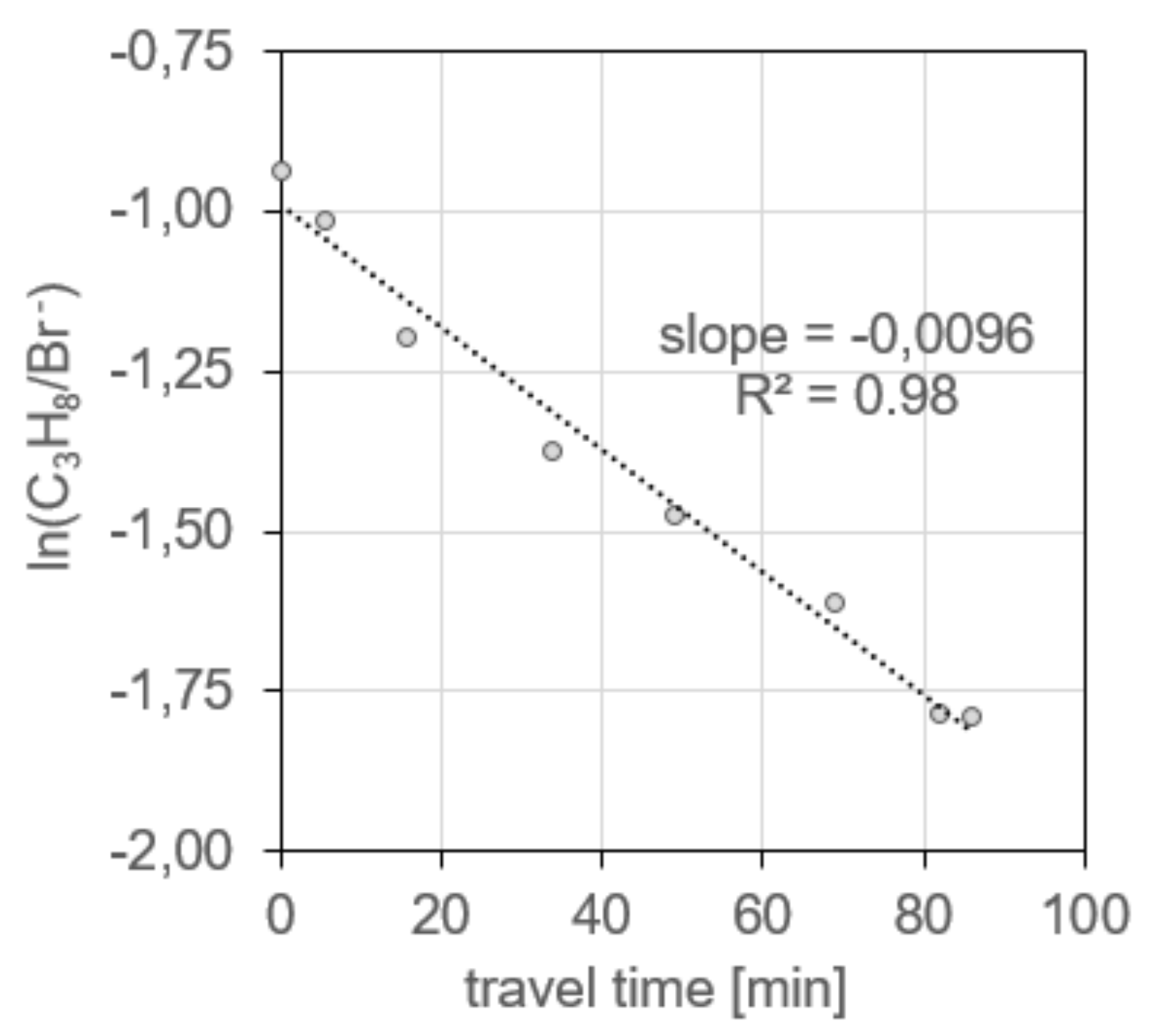
2.2.2. Determination of the Radon Degassing Rate

While radon loss by decay is exactly quantifiable based on the radon half-life, the determination of its loss by degassing to the atmosphere is more involved. Hence, the radon degassing rate is one of the largest uncertainties in radon mass-balances for stream sub-reaches [14].

Gas exchange between surface waters and the atmosphere has been investigated in a considerable number of studies with differing purposes. Early investigations focused on re-aeration of surface water bodies, i.e., on oxygen enrichment of the water column. Later studies introduced approaches that aimed to quantify greenhouse gas exchange (CO₂ and CH₄) across the air/water interface as well as gross stream ecosystem productivity [15,16,17]. Comparable approaches can be used for evaluating radon degassing from surface waters to the atmosphere.

Radon degassing is primarily driven by turbulence in the stream water column, which reduces the thickness of the stagnant boundary layer at the water–air interface (e.g., [18,19]). Turbulence, in turn, is dependent on many factors, such as stream geometry (width, depth and slope), bed roughness and flow velocity. Consequently, shallow and turbulent headwater streams show a much more intense and much less quantifiable degassing than major rivers.

Generally, gas loss from streams can be quantified with the gas specific degassing coefficient (k, (d⁻¹)) (also called piston velocity or re-aeration coefficient). Many empirical equations relate stream physical properties to gas exchange and hence to gas-specific values of k (see compilation in [20]). As briefly mentioned above, these empirical approaches tend to work well in systems similar to those where they were derived, which are usually larger streams and rivers. However, they tend to particularly fail in small headwater streams [21]. This is thought to be due to scaling problems in turbulence generation between rivers and small rivulets.

Because of this general difficulty in degassing determination, we applied and compared the results of two experimental and two empirical methods to estimate k_Rn for the 1050 m profile of the Schaefetal rivulet. Besides, a better evaluation of the respective site-specific results this multi method approach allowed a comparison of the techniques, i.e., a general evaluation of their advantages and disadvantage in small headwater studies.

During the low-flow campaign (i.e., the first campaign), we estimated k_Rn experimentally based on the decrease in radon concentration over the losing sub-sections of the rivulet [22]. The method assumes that there is no groundwater discharge within the losing sub-sections and that all radon concentration decrease is due to degassing (radioactive decay can be neglected over these very short time scales). Since the resulting degassing coefficient is based on a fit of the radon concentration profile over the losing sub-sections, we call it k_Rn-fit. We compared the measurement data based k_Rn-fit with the results of two empirical equations (k_Rn-emp1 and k_Rn-emp2) from the compilation of Parker and Gay [20], which are both based on the stream velocity (v [m d⁻¹]) and the stream depth (d [m]). The first empirical equation (Equation (1)) was originally from [23], and the second (Equation (2)) from [24]. Note that both these equations have been scaled from feet to meters and from O₂ to radon [25].

$${\mathrm{k}}_{\mathrm{Rn}-\mathrm{emp}1}=9.301\times {10}^{-3}\left(\frac{{\mathrm{v}}^{0.5}}{{\mathrm{d}}^{1.5}}\right)$$

(1)

$${\mathrm{k}}_{\mathrm{Rn}-\mathrm{emp}2}=4.87\times {10}^{-4}{\left(\frac{\mathrm{v}}{\mathrm{d}}\right)}^{0.85}$$

(2)

In our high-flow campaign (i.e., our second campaign), we additionally used a propane injection approach that allowed determining radon degassing experimentally (k_Rn-meas) by actual onsite propane degassing measurement. The propane approach could not be applied during the low-flow campaign because the low rivulet water level did not allow sound propane injection.

While propane has been used to quantify stream/atmosphere exchange since the 1970s (e.g., [15,26]), the approach has seldom been applied for quantifying radon degassing from streams as part of a radon mass-balance ([10,25]). In the high-flow campaign, the propane was added to the rivulet at the upstream end of the investigated reach at a constant rate of through an Accurel tube (PP V8/2) that was fixed to the streambed. The 20 L min⁻¹ injection rate was adjusted by means of a pressure regulator. Once the propane concentration had reached steady state along the investigated 1050 m profile, water samples (5 mL) were taken at eight stations using gas-tight glass syringes. In the laboratory (~4 h after sampling), 5 mL of air were brought into the syringe, shaken for 1 min and left standing for 5 min. The headspace was then injected into previously evacuated headspace vials. The propane concentration was quantified by gas chromatography–flame ionization detection (GC-FID) after calibration with known high purity propane standards. The decrease in propane from station to station was used to calculate the propane degassing coefficient “k_p”. To account for any propane concentration dilution along the profile, bromide was released simultaneously to the propane to the rivulet as conservative tracer (cf. Section 2.2.5). Using the resulting data, k_p was calculated for each sub-section of the 1050 m profile as:

$${\mathrm{k}}_{\mathrm{p}}=\frac{1}{\mathsf{\tau }}\ln \left(\frac{{\left[{\mathrm{C}}_3{\mathrm{H}}_8\right]}_{\mathrm{U}}\times {\mathrm{Br}}^{-}{}_{\mathrm{D}}}{{\left[{\mathrm{C}}_3{\mathrm{H}}_8\right]}_{\mathrm{D}}\times {\mathrm{Br}}^{-}{}_{\mathrm{U}}}\right)$$

(3)

where τ is the travel time [h] between the injection point and the downstream sampling station; U and D indicate adjacent upstream and downstream stations of the sub-section, respectively; C₃H₈ is the propane concentration in the stream water [mg l⁻¹]; and Br⁻ is the steady state bromide concentration in the stream water [mg l⁻¹].

If there are no sudden substantial concentration changes along the complete profile, k_p can (alternatively to Equation (3)) also be calculated as the slope of the linear regression line of ln(C₃H₈/Br⁻) vs. travel time [27]. This approach produces an average propane specific degassing coefficient for the whole stream reach.

Finally, the achieved propane specific k_p needs to be scaled to the radon specific k_Rn-meas. This was done by using the ratio of the Schmidt numbers of the two gases:

$${\mathrm{k}}_{\mathrm{Rn}-\mathrm{meas}}={\mathrm{k}}_{\mathrm{p}}\times \left(\frac{{\mathrm{Sc}}_{\mathrm{Rn}}}{{\mathrm{Sc}}_{\mathrm{P}}}\right){}^{\mathrm{n}}$$

(4)

where Sc_Rn and Sc_P represent the Schmidt numbers of radon and propane, respectively. The exponent n depends on the degree of turbulence and ranges between −1/2 and −2/3, with lower values for more turbulent conditions [18]. We used a value of 1/2 as most consistent with a shallow turbulent rivulet. The Schmidt number for propane was calculated as in [28], also including a temperature correction to 5 °C for the rivulet water during the high-flow campaign. The Schmidt number for radon was calculated as the ratio between the kinematic viscosity to the molecular diffusion coefficient, both scaled to 5 °C. The resulting Schmidt number ratio Sc_Rn/Sc_P was ~0.73 and the correction factor (Sc_Rn/Sc_p)^−0.5 was 1.16.

It should be kept in mind however that Equations (1) and (2) were set up for radon degassing from major rivers (as mentioned above) and that scaling problems to small (turbulent) rivulets might exist. Furthermore, there are uncertainties when extrapolating the propane experiment data to radon. This includes the made assumptions about hydrology and river geometry as well as the scaling from propane to radon (cf. Section 4).

2.2.3. Determination of ²²⁶Ra in River Sediments

²²²Rn is permanently produced by the decay of ²²⁶Ra in the sediment of the rivulet. To evaluate the radon equilibrium concentration of the sediment pore water as potential radon source, three sediment samples were taken for determination of the ²²⁶Ra activity concentration. The analyzed sample material represented the rivulet sediments within the studied reach of the watercourse. The radium activity concentration was measured using an ORTEC-Gamma-X HPGe coaxial low-energy n-type detector (ORTEC AMETEK; Oak Ridge, Tennessee, United States). Detector and measuring geometry were calibrated using the certified IAEA reference material RGU-1. The radium activity concentration was determined based on the distinct gamma emission energies of the short-lived radon progeny ²¹⁴Pb (295.2 and 351.9 keV) and ²¹⁴Bi (609.3 and 1120.3 keV) with a mean standard deviation of 5%. To ensure decay equilibrium between radium and short-lived radon progeny, the samples were stored before measurement for 27 days (seven ²²²Rn half-lives) in the radon-tight capsules that were placed on the detector for measurement.

2.2.4. Radon Determination in Groundwater and Surface Water

For groundwater endmember determination of radon, samples were taken from three groundwater wells located close to the rivulet and two subsurface agricultural drainages. For radon mapping along the rivulet, samples were taken from six locations distributed equidistantly between the gauging station (Point #0) and the end of the profile 1050 m upstream of it (Point #5) (cf. Figure 1). The water samples from the wells (n = 3), the drainages (n = 2) and the rivulet (n = 6) were transferred into a stripping unit avoiding turbulence and thus minimizing degassing during the sampling process. Radon on-site measurement was executed as described by Schubert et a l. [2] using the radon-in-air monitor AlphaGuard (Bertin Technologies, Montigny-le-Bretonneux, France). The recorded radon-in-air values were converted into radon-in-water concentration allowing for the radon partition coefficient as described by [19].

2.2.5. Rivulet Discharge Determination

For the two field campaigns, two common tracer approaches were applied for determining the discharge of the rivulet [L s⁻¹]. During the low-flow campaign, the discharge was derived from salt pulse tracer injections at six locations along the rivulet (#5–#0; cf. Figure 1). All measurements were done using electric conductivity probes (CTD divers), which had been calibrated to allow converting the measurements into Cl- concentrations based on a linear relationship. For each measurement, 500 g sodium chloride were dissolved in 2 L of rivulet water and injected as a slug into the rivulet 20 m upstream of the respective location. Discharge was derived as the ratio of added tracer mass and integrated tracer flux. The tracer flux was quantified based on the detected concentration breakthrough curve at the respective station. The tracer breakthrough was also measured at the next downstream location, which allowed deriving the fractional tracer loss for each sub-section.

During the high-flow campaign, a continuous and constant upstream bromide injection (Q_Br) was executed as part of the propane degassing experiment (cf. Section 2.2.2). The resulting bromide dataset could also be used for rivulet discharge determination (making further salt pulse tracer injections dispensable). Bromide was added to the rivulet at a rate of 650 mL min⁻¹ 15 m upstream from the uppermost sampling point (Point #5). Once steady state was reached over the complete length of the investigated 1050 m profile, the rivulet discharge Q_Br [L s⁻¹] was calculated by:

$${\mathrm{Q}}_{\mathrm{Br}}=\frac{{\mathrm{Br}}^{-}{}_{\mathrm{inject}}\times {\mathrm{Q}}_{\mathrm{in}}}{\left[{\mathrm{Br}}_{\mathrm{stream}}^{-}\right]-\left[{\mathrm{Br}}_{\mathrm{back}}^{-}\right]}$$

(5)

where Br⁻_inject is the bromide concentration in the injection fluid, Br⁻_stream [mg L⁻¹] is the bromide concentration in the rivulet water at steady state, Br⁻_back [mg L⁻¹] is the background bromide concentration in the rivulet and Q_in is the rate of tracer injection to the rivulet [L s⁻¹].

In addition to the two described tracer approaches, the rivulet discharge was also measured physically as point value by the weir at the catchment outlet. The resulting data were a suitable measure for evaluating the reasonability of the tracer results.

2.3. Processing of the Field Data with FINIFLUX

Groundwater discharge to the rivulet was quantified using a steady state mass balance for in-stream radon for each of the five sub-sections of the 1050 m profile. The mass balance was calculated using the FINIFLUX model, which is described in detail in [15]. FINIFLUX numerically solves the mass balance equation for in-stream ²²²Rn at the reach scale by using a Petrov-Galerkin Finite Element scheme based on on-site radon measurement results (Equation (6)). Groundwater discharge was calculated individually for each of the five sub-sections between the six radon sampling stations Point #5 (upstream) and Point #0 (downstream gauging station).

$${\mathrm{Q}}_{\mathrm{s}}\frac{\mathrm{dc}}{\mathrm{dx}}=\mathrm{I}\left({\mathrm{c}}_{\mathrm{gw}}-\mathrm{c}\right)-\mathrm{kwdc}-{\mathrm{dwc}\mathsf{\lambda }}_{\mathrm{Rn}}+{\mathsf{\alpha }}_1-{\mathsf{\alpha }}_2\mathrm{c}+\frac{{\mathrm{Q}}_{\mathrm{r}}}{{\mathrm{R}}_{\mathrm{L}}}\left({\mathrm{c}}_{\mathrm{trib}}-\mathrm{c}\right)$$

(6)

where x [m] is the length of the investigated sub-section, w [m] is its mean width and d [m] is its mean depth. I [m³ m⁻¹ d⁻¹] is the groundwater discharge rate within the sub-section, i.e., the parameter of interest. Q_s [m³ d⁻¹] is the discharge of the rivulet. c and c_gw [Bq m⁻³] are the ²²²Rn activities in the rivulet water specific for the sub-section and the overall groundwater endmember, respectively. The parameter k [d⁻¹] is the degassing coefficient and λ_Rn [d⁻¹] is the first-order decay constant for ²²²Rn. Q_r [m³ d⁻¹] is the inflow from tributaries within the sub-section, R_L [m] is the mean width of the tributaries where they enter the investigated stream and c_trib [Bq m⁻³] is the mean ²²²Rn activity in the tributaries. Since there are no tributaries to the Schaefertal rivulet, the last three parameters were neglected. (The water discharge rate from the two drains was negligible.) The parameters α₁ and α₂ quantify hyporheic exchange. They depend on the physical characteristics of the hyporheic zone and its residence time distribution, i.e., hyporheic depth and mean residence time. The related details on the definition of α₁ and α₂ are discussed in Pittroff et al. [29] and Frei et al. [30].

The modeled radon profile (Equation (6)) was fitted to the measured radon data by varying: (i) the groundwater discharge rate; (ii) hyporheic depth; and (iii) hyporheic mean residence time. This fitting process was done using the BeoPEST code [31].

3. Results

3.1. Radon Degassing Rate

Table 1. Degassing coefficients determined for the investigated 1050 m profile of the Schäfetal rivulet. The k_Rn-emp values are the averaged results from all five sub-sections.

Evaluation Method	kRn Low-Flow Campaign [d−1]	kRn High-Flow Campaign [d−1]
Radon fitting (kRn-fit)	27.0	33.0
Empirical Equation (1) (kRn-emp1)	10.4	7.9
Empirical Equation (2) (kRn-emp2)	5.5	5.9
Propane experiment (kRn-meas)	not executed	15.9

summarizes the radon losses to the atmosphere based on degassing coefficients (k) derived from the decrease in radon activity over losing sub-sections (k_Rn-fit), two independent empirical models (k_Rn-emp1 and k_Rn-emp2) and the propane degassing experiment (k_Rn-meas, high-flow campaign only).

The fitting of radon losses resulted in coefficients of k_Rn-fit = 27 d⁻¹ and k_Rn-fit = 33 d⁻¹ for the low-flow campaign and the high-flow campaign, respectively. The two empirical models produced k_Rn-emp coefficients ranging between 10.4 and 5.5 d⁻¹, depending on equation and campaign. The propane degassing experiment showed an exponential decrease in propane concentrations with travel time (and distance) without any sudden changes (see Supplementary Materials: “Results from propane experiment”). Hence, we calculated a single propane degassing coefficient k_p from the slope of the linear regression line (Figure 2). Converting k_p into k_Rn-meas resulted in a radon degassing rate of k_Rn-meas = 15.9 d⁻¹.

3.2. Radon Production in the Sediment by ²²⁶Ra Decay

The detected mean ²²⁶Ra activity of the three sediment samples was A_Ra = 30 ± 5 Bq kg⁻¹. With a measured sediment dry density of ρ = 1200 kg m⁻³, an assumed emanation coefficient of the material of ε = 0.24 [32] and a measured sediment pore space of n = 0.4, this radium activity yields theoretically a radon pore water concentration of C_Rn = 21.6 ± 3.6 kBq m⁻³ (Equation (7)).

$${\mathrm{C}}_{\mathrm{Rn}}=\frac{{\mathrm{A}}_{\mathrm{Ra}}\times \mathsf{\epsilon }\times \mathsf{\rho }}{\mathrm{n}}$$

(7)

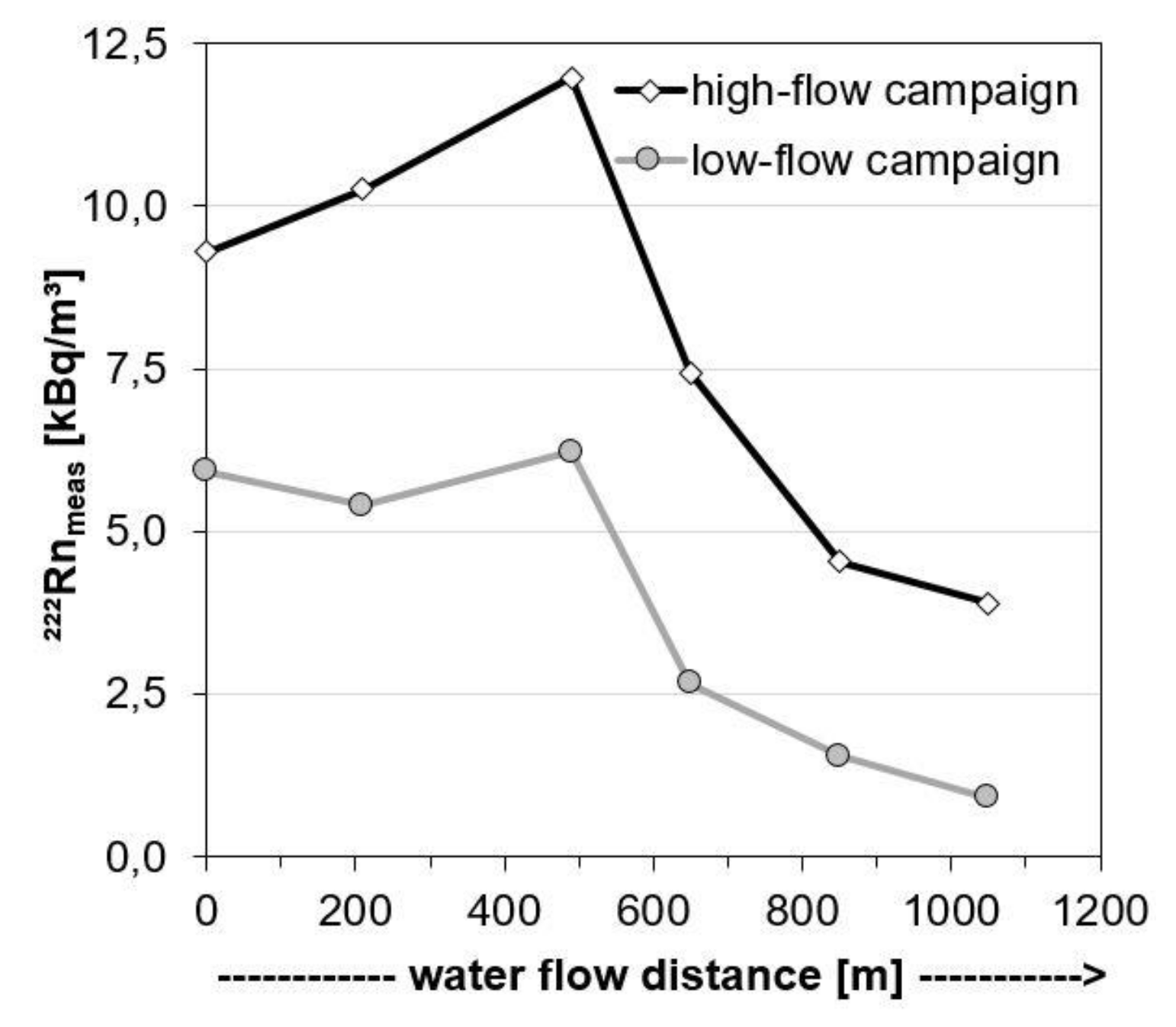
3.3. Radon Concentration in Groundwater and Rivulet Water

Groundwater: The two drainage water samples can be considered representative for groundwater because no radon degassing occurs within the subsurface drainage system, since the headspace air in the system is in radon partition equilibrium with the constantly flowing drain water. Interaction with the outside air at the discharge point of the system is negligible. The resulting groundwater endmember (n = 5) revealed a radon concentration of about 23.2 ± 1.4 kBq m⁻³ (

Table 2. ²²²Rn activity concentrations in groundwater (GW) and rivulet water samples (Points #5–#0) detected during two sampling campaigns; all activity concentrations in [Bq m⁻³].

	22 January 2019	13 February 2019
Drainage mean	23,210 ± 1138
GW mean	23,243 ± 1696
Point #5	5924 ± 129	9300 ± 657
Point #4	5403 ± 052	10,265 ± 695
Point #3	6227 ± 193	11,983 ± 732
Point #2	2671 ± 160	7447 ± 509
Point #1	1543 ± 062	4532 ± 348
Point #0	915 ± 043	3903 ± 318

). This concentration comes close to the radon pore water concentration of 21.6 kBq m⁻³ calculated based on the mean ²²⁶Ra activity of the sediment samples. Hence, 23.2 ± 1.4 kBq m⁻³ could be considered a reasonable value and was used as groundwater endmember for further mass-balance modeling.

Rivulet water: The radon concentration profile along the rivulet (Rn_meas, n = 6, Table 2) showed a distinct gradient with higher (or even rising) concentrations in the two upstream and declining concentrations in the three downstream sub-sections (Figure 3) of the 1050 m profile. This overall pattern was similar during both sampling campaigns. However, significantly higher concentrations were observed in the high-flow campaign, with radon activities being approximately double that observed in the low-flow campaign.

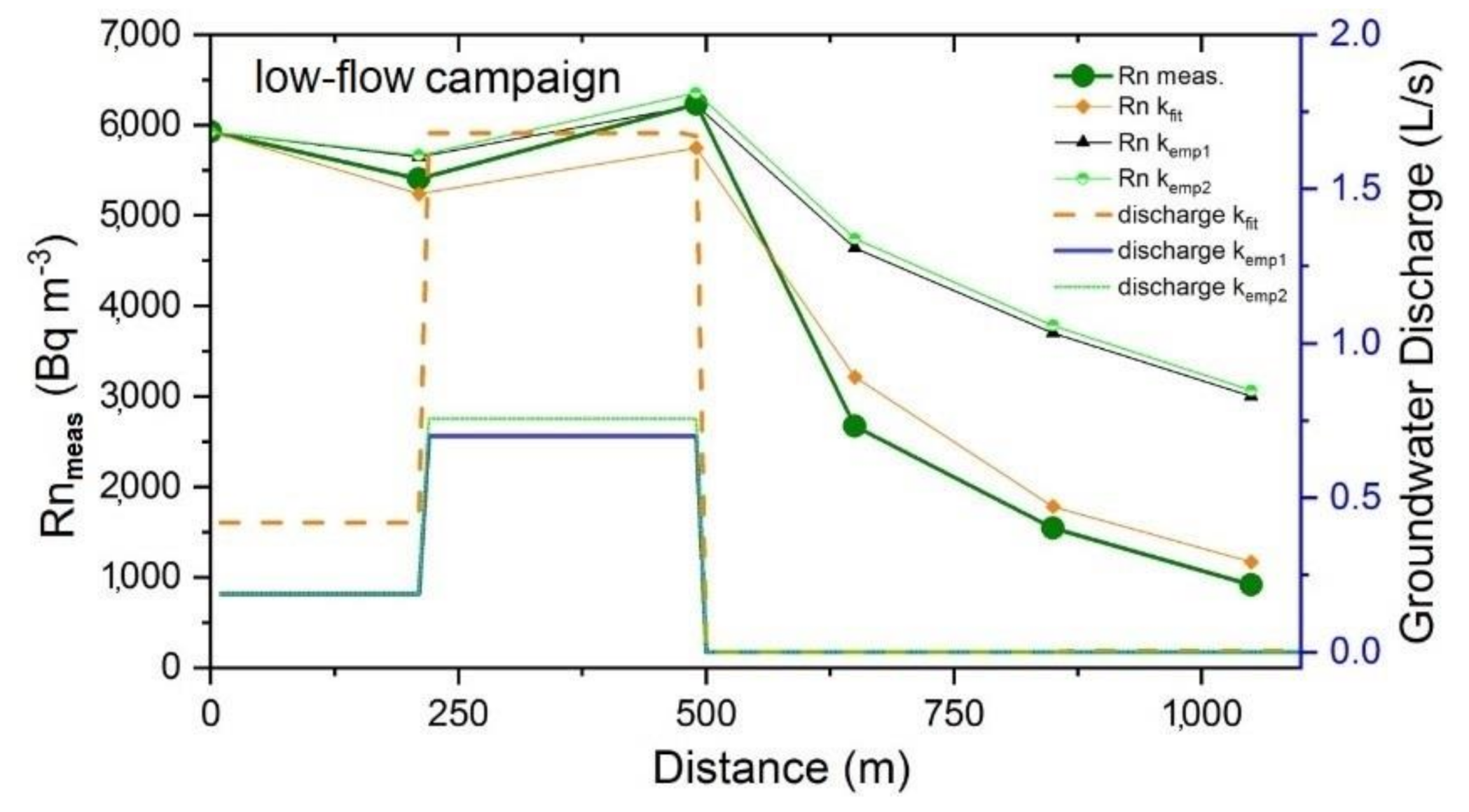
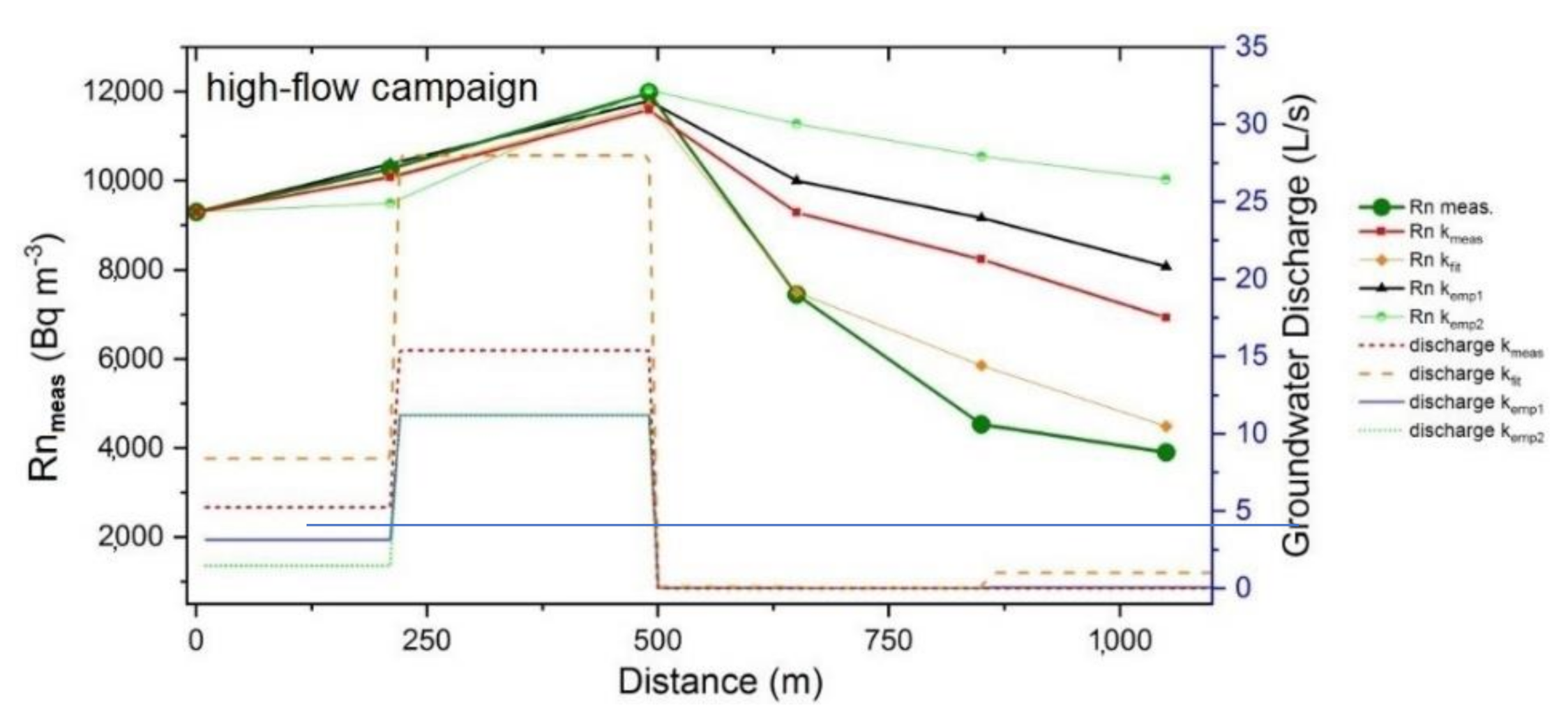
3.4. Groundwater Discharge Localization and Quantification Using FINIFLUX

Low-flow campaign (see Supplementary Materials: “Parameters used for FINIFLUX simulations”): The groundwater discharge rates that result from the FINIFLUX model for the five sub-sections of the 1050 m profile are displayed in Figure 4. The three discharge plots calculated based on the degassing coefficients k_Rn-fit, k_Rn-emp1 and k_Rn-emp2 show consistently that the majority of groundwater discharge occurred in the upper two sub-sections of the profile. At the same time, the two radon concentration profiles modeled based on the empirical parameters k_Rn-emp1 and k_Rn-emp2 show that these parameters strongly underestimate radon loss by degassing; the two plots only poorly capture the measured decrease in radon concentration (Rn_meas) over the three sub-sections downstream. Only the radon concentration profile modeled based on k_Rn-fit resembles the measured radon profile. This is expected however as k_meas is part of the fitting process.

The exponential decrease in Rn_meas in the three downstream sub-sections indicates degassing as the dominant radon sink and very little to no groundwater discharge. Given that the geometry of the stream (depth and width) was relatively constant, a linear or a polynomial radon trend would rather have pointed toward a substantial impact of processes other than degassing such as groundwater discharge, hyporheic flux or contribution of tributaries.

The groundwater discharge rates that were modeled individually for each of the five sub-sections as displayed in Figure 4 were compared to the net water gain to the 1050 m rivulet profile as determined based on the salt pulse tracer data. While the FINIFLUX run based on k_Rn-fit resulted in a cumulative net groundwater discharge of 2.1 L s⁻¹, the salt tracer data showed a net water gain of 1.2 L s⁻¹. The two model runs based on the seemingly unsuitable empirical parameters k_Rn-emp1 and k_Rn-emp2 produced cumulative net groundwater discharge ranging from 0.6 to 0.9 L s⁻¹.

High-flow campaign (see Supplementary Materials: “Parameters used for FINIFLUX simulations”): The groundwater discharge rates for the five sub-sections that result from the FINIFLUX model are displayed in Figure 5. As for the low-flow campaign, all model approaches consistently indicate groundwater discharge in the upper two sub-sections. Furthermore, k_Rn-emp1 and k_Rn-emp2 again underestimate degassing in the lower sections, i.e., they were not able to account for the rapid radon concentration decrease over the three downstream sub-sections. Surprisingly, the degassing value calculated from the propane experiment (k_Rn-meas) was also not sufficient to account for the radon decrease in the three lower sub-sections of the profile. Only the k_Rn-fit value was able to produce a reasonable model fit to the measured data, again as expected due to the inclusion of Rn_meas in the fitting process. However, the good model fit based on k_Rn-fit was at the expense of the water balance. While the overall net water gain based on the bromide data was ~13.5 L s⁻¹ (i.e., about ten times as high as during the low-flow campaign), the cumulative groundwater discharge as estimated by FINIFLUX based on k_Rn-fit was 37 L s⁻¹, i.e., overestimating groundwater discharge by a factor of about three. The model run based on k_Rn-emp1 gave a cumulative discharge of 16 L s⁻¹, k_Rn-emp2 gave a discharge of 13 L s⁻¹ and k_Rn-meas resulted in a groundwater discharge of 22 L s⁻¹. This shows that in particular the empirical equations came close to the measured water balance despite the pore model fit to radon in the lower sections of the streamlet.

Each k value (for both campaigns) was systematically varied by ±25% to estimate how sensitive the modeled groundwater discharge was to uncertainties of k in the individual degassing models. For the low flow campaign, the resulting calculated cumulative groundwater discharge ranged 0.75–1.13 L s⁻¹ using k_Rn-emp1 and 0.42–0.65 L s⁻¹ for k_Rn-emp2 with the higher discharge rates associated with larger k values. This ± 25% change in k corresponds to a relative uncertainty ranging between ca. 12% and 28%. For the high-flow campaign, the same calculation gave groundwater discharge rates of 13.2–17.9 L s⁻¹ for k_Rn-emp1, 11.8–15.0 L s⁻¹ for k_Rn-emp2 and 19.6–26.4 L s⁻¹ for kRn-meas. This corresponds to a relative change in the groundwater discharge rate ranging between about 10% and 19% (

Table 3. Error propagation evaluation of the degassing coefficient (k). The displayed values show the groundwater discharge rates (I) [L s⁻¹] resulting from the degassing coefficients (k) used in the model and changed by ± 25%.

		−25%	Used Value	25%
low-flow	kemp1	0.75	0.9	1.13
	%	−16.7		25.6
	kemp2	0.42	0.6	0.65
	%	−27.6		12.1
high-flow	kemp1	13.2	16.3	17.9
	%	−19.0		9.8
	kemp2	11.8	13.2	15.0
	%	−10.6		13.6
	kmeas	19.6	22.6	26.4
	%	−13.3		16.8

).

4. Discussion

4.1. Site-Specific Results

Low-flow campaign: Despite not fitting the measured radon data (Rn_meas) in the three lower sub-sections, the cumulative groundwater discharge calculated based on the two empirical parameters (k_Rn-emp1 and k_Rn-emp2) gave plausible water fluxes. The results suggest that ~75% of the water gained to the rivulet along the 1050 m profile was derived from groundwater. In contrast, the cumulative groundwater discharge based on k_Rn-fit was 175% of the water gain derived from the salt tracer data. Even though the latter two results differ significantly in relative numbers, one has to consider that the difference in absolute values is only 0.9 L s⁻¹. (1.2 vs. 2.1 L s⁻¹). Three potential explanations can be given for this (in absolute values) slight overestimation of the FINIFLUX model based on k_Rn-fit.

A first general reason is the uncertainties of the input data. A second potential explanation is that some of the rivulet water is temporarily infiltrating the hyporheic zone, accumulating radon on its subsurface flow path and re-emerging further downstream. Such hyporheic exchange will be interpreted by FINIFLUX as groundwater discharge, while there is no net change for the water balance. Such effects on the radon balance have been observed in braided rivers with a large proportion of parafluvial flow [33,34]. While this has not been systemically investigated for radon in headwater catchments, it is known that such minor streams have a large proportion of water flowing through the hyporheic zone due to: (i) relatively large in-stream hydrological gradients; (ii) turbulent conditions; and (iii) a large stream bed to discharge ratio [35,36]. Indeed, Liao et al. [37] showed in a small headwater stream in southern Germany that the entire stream water passes through the hyporheic zone at least once over a 200 m reach. As a third explanation, it is possible that degassing is not uniform over the investigated profile of the rivulet. It could be assumed that the degassing value estimated for the three losing sub-sections downstream is not representative for the two gaining upstream sub-sections (where potentially less radon is lost by degassing), thus overestimating the degassing there and requiring higher groundwater discharge to compensate the modeled radon loss to the atmosphere.

High-flow campaign: The radon concentrations during the high-flow campaign were double that of the low-flow campaign. This suggests that groundwater was contributing a significant proportion of the total flow in the rivulet. This could be due to pressure loading of snowmelt water on the shallow aquifer, pushing “old” (residence time longer than ~20 days) riparian groundwater into the rivulet.

Generally, the modeling of the high-flow campaign proved more difficult than the low-flow campaign discussed above. The strong discrepancy between net water gain based on the bromide data and the cumulative groundwater discharge based on k_Rn-fit (13.5 vs. 37 l s⁻¹) cannot be explained with statistical uncertainties of the input data alone. The second explanation discussed for the low-flow campaign assuming rivulet water infiltrating the hyporheic zone and re-emerging further downstream also seems rather unlikely. In contrast to the low-flow campaign, where this explanation was reasonable, there is no evidence of the required substantial interaction in the downstream sub-sections. The third explanation given for the low-flow campaign is not reasonable either, since it is not supported by the propane experiment, which showed relatively uniform degassing over the complete 1050 m profile.

With these three explanations being not satisfactory, we consider it likely that radon in the rivulet is significantly diluted in the lower three sub-sections by (practically radon-free) surface-near interflow and surface water runoff due to the preceding rain and the recent snowmelt. Such water flow can be expected to occur spatially homogeneously and does hence not result in any abrupt radon concentration decrease. However, the concentration decrease results in an overestimation of radon degassing and hence in an overestimation of the discharging groundwater volume required for its compensation in the radon mass balance.

We have to admit that the latter explanation is also somewhat unsatisfactory. However, at the present time, we have no alterative way of accounting for the rapid loss in radon in the mass-balance and prefer the surface water runoff idea for maintaining the water balance.

The groundwater discharge modeled with k_Rn-mean also exceeded the water balance. The reasons for this discrepancy may be similar to those given above or from difficulties in scaling propane degassing to radon degassing using the Schmidt number. The temperature correction for the Schmidt number for each gas is likely to be associated with a significant uncertainty as it is based on empirical relationships between temperature and Schmidt number values, with reference temperatures commonly being between 20 and 25 °C [28].

In contrast to the unreasonably high groundwater discharge rate based on k_Rn-fit, there was a good agreement between the bromide-based results and the cumulative groundwater discharge rates based on k_Rn-emp1 and k_Rn-emp2 (13.5 vs. ~13–16 L s⁻¹). This supports the assumption that some process such as concentration dilution by snowmelt is decreasing the radon concentration in the rivulet water on top of degassing.

4.2. General Results

The sensitivity of groundwater discharge estimations to the used model parameters depends generally on the used model [22,38]. Besides the site-specific and campaign-specific results presented above, the outcome of the study allows general conclusions regarding the sensitivity of the individual FINIFLUX model parameters and their impact on the model results, i.e., on the general strengths and weaknesses of the FINIFLUX approach for small headwater streams. The site-specific input parameters of the FINIFLUX model that are required for the qualitative and quantitative evaluation of groundwater discharge into streams include the following (cf. Equation (6)):

(i)

The dimensions of the stream sub-section in question (and of its potential tributaries)

(ii)

The water discharge rate of the stream within this sub-section (and of the potential tributaries)

(iii)

The sub-section specific ²²²Rn concentration in the stream water (and in potential tributaries)

(iv)

The radon groundwater endmember representative for the hydraulically connected aquifer

(v)

The sub-section specific radon degassing coefficient

Generally, the stream dimensions of major rivers are known. The information can in most cases be requested from local authorities or attained from satellite data. The situation is different for minor streams or headwater rivulets. Width and depth data have to be measured or estimated in the field. Furthermore, while the stream dimensions of major streams may vary over short distances by only a few percent, such relative changes can be much more pronounced in small streams. Hence, the stream dimensions assumed for modeling a sub-reach of a minor stream might reflect the real situation only vaguely. In particular, headwater (or any small) rivulets are sensible in this regard. The width or depth might change by 50% or more over short distances, which makes it more difficult to define the input parameters.

The situation is comparable for the river water discharge rate. For major rivers, it is continuously monitored at readily installed gauging stations, and the data are generally freely available. On the other hand, discharge rates are in general not monitored for minor streams and rivulets, which react, on top of this, much more sensibly to varying environmental situations. Stream water that is infiltrating the hyporheic zone and re-appearing, after a certain distance of subsurface flow, is likely but at the same time difficult to detect. However, rivulet discharge rates can be determined with minor effort using standard methods. In our case, it was determined: (i) in the sub-sections using salt pulse tracer injections and continuous bromide injections; and (ii) overall at the gauging station. The resulting data are consistent and reliable.

Regarding the measurement of the river water radon concentration, the situation is advantageous for smaller watercourses. In contrast to major rivers, where an incomplete mixing of stream water and discharging groundwater along river sections might be a source of error for representative river water sampling [39,40], such incomplete mixing is much less likely in turbulent small rivulets. Hence, representative radon concentration mapping along small headwater streams is generally possible with low statistical uncertainty in the results. In the given case, the radon concentration in the rivulet was measured on site with the reported uncertainties (cf. Table 2).

A sensitive parameter that is in general (and independently from the river size) less unequivocal to define is the local radon groundwater endmember [41,42,43]. Site-specific values can be spatially variable due to small-scale changes in the local aquifer geology. A statistically reliable value therefore requires data input from as many independent sources as possible. Such sources include: (i) potentially existing datasets collected by, e.g., water authorities or water providers, an option that is more likely in the case of major rivers; (ii) calculations based on the ²²⁶Ra activity of aquifer or sediment material (based on reasonable values for radon emanation coefficient and density/porosity of the mineral matrix; cf. Equation (7)); and (iii) measurements of water samples taken from wells, springs or drainages that tap the aquifer in question. In the study presented here, groundwater endmembers were estimated from well water (²²²Rn), drainage water (²²²Rn) and sediment measurements (²²⁶Ra) with consistent results (cf. Section 3.2 and Section 3.3). If the results of an investigation turn out to be more diverse, which tends to be the case in larger catchments than the Schaefertal, the appropriateness of the datasets must be evaluated individually in view of the data source reliability and the site-specific conditions.

As most critical model parameter of the FINIFLUX approach when applied for small and turbulent headwater streams, our study revealed the radon degassing coefficient. The difficulty of defining the most suitable degassing coefficient is reflected in Section 3.4. While all other model parameters could be determined with satisfying uncertainty, the assumed degassing coefficient used for the modeling is rather poorly constrained and, at the same time, has a high impact on the radon mass-balance. This can be seen by the sensitivity analysis, where a ±25% change in the k value can lead to between 10% and 27% difference in the calculated groundwater flux. As for the radon groundwater endmember, it is therefore mandatory to include as many data sources or detection approaches as possible to reduce the uncertainty associated with quantifying the degassing. Potential options include: (i) applying empirical equations; (ii) attributing detected radon losses in (verifiably) losing stream sections exclusively to radon degassing; and (iii) degassing experiments based on upstream gas injections. While the latter approach appears to be the most promising one because it is based on direct measurements, it includes the challenge of incorrect scaling from the tracer gas loss (in our case propane) and radon loss coefficients. Scaling the gas loss coefficients is based on empirical relations (cf. Equation (4)). The empirical equations use the Schmidt numbers of the gasses as essential data, a dimensionless number defined as the ratio of dynamic viscosity and mass diffusivity. Similar Schmidt numbers indicate that momentum and mass transfer by diffusion (i.e., gas loss) are comparable, and that concentration boundary layers are similar. However, while mass diffusion in liquids grows with temperature, viscosity behaves roughly inversely proportional with temperature, so that the Schmidt number quickly decreases with temperature. Hence, the empirical assumptions made might be inaccurate, especially at unusually low water and air temperatures as during our sampling campaigns. Hence, even if a wide range of independent datasets were available, the resulting degassing rate could still be inconclusive (cf. Table 1). In such a case, the reasonability of the individual datasets must be evaluated in view of the specific circumstances of the site (morphology of the streambed, intensity of water turbulence and assumptions in the model used), the time of sampling (season and hydrological situation) and finally the own experience. Furthermore, it might be advisable to adapt the overall degassing coefficient, as determined for the whole investigated stream section, sub-section-wise based on obvious small-scale changes in stream characteristics (turbulence, width and depth).

5. Conclusions

Two field campaigns were carried out under strongly different hydrological conditions along a well-defined 1050 m section of a small headwater stream. While the first campaign (low-flow campaign) took place under hydrological drought low-flow conditions, the second campaign (high-flow campaign) was characterized by recent rains and snowmelt triggering a high rivulet discharge and increased interflow and surface water runoff into the rivulet.

The overall study aimed at: (i) a site-specific evaluation of groundwater discharge into the investigated section of the rivulet; and (ii) a general evaluation of the applicability of the FINIFLUX approach for small headwater streams. Accordingly, the results of the study revealed the following conclusions.

(i)

Specifically: The groundwater discharge areas along the investigated section of the rivulet that were suggested by earlier hydrological modeling of the site [12] could be confirmed using radon measurements and mass-balance calculations with FINIFLUX. Groundwater discharge zones could be localized and discharge fluxes quantified, despite significant uncertainty in parameterizing radon degassing in the FINIFLUX model.

(ii)

Generally: In contrast to conventional hydrological modeling, the FINIFLUX approach is based on a combination of real tracer data (radon, Br⁻ and propane) and mass-balance modeling. This adds certainty that the distributed highly parameterized process-based modeling is representing the field site realistically. However, in the case of groundwater discharge localization and quantification in small headwater streams, the model is only suitable when the required parameters can be well constrained. While most required input parameters are attainable with reasonable statistical certainty, the determination of reliable values for the following is challenging, but at the same time critical for reliable estimates of groundwater fluxes: (i) the radon groundwater endmember; and (ii) the radon degassing coefficient. In particular, estimation of the radon degassing rate requires a site-specific critical assessment of the reasonability of the used datasets and the resulting outcomes. The determination of both radon groundwater endmember and radon degassing coefficient should hence not rely on only vague estimations or single data sources but be based on as many as possible data sources.

References

1. Fleckenstein, J.H.; Krause, S.; Hannah, D.M.; Boanom, F. Groundwater-surface water interactions: New methods and models to improve understanding of processes and dynamics. Adv. Water Resour. 2010, 33, 1291–1295. [Google Scholar] [CrossRef]
2. Schubert, M.; Knöller, K.; Treutler, H.C.; Weiß, H.; Dehnert, J. On the Use of Naturally Occurring Radon-222 as Tracer for the Estimation of the Infiltration of Surface Waters into Aquifers. In Radioactivity in the Environment Vol. 8—Radioactivity in the Environment; Povinec, P., Sanchez-Cabeza, J.A., Eds.; Elsevier Book Series: Amsterdam, The Netherlands, 2006; pp. 326–334. [Google Scholar]
3. Hutchinson, P.A.; Webster, I.T. Solute Uptake in Aquatic Sediments due to Current-Obstacle Interactions. J. Environ. Eng. 1998, 124, 419–426. [Google Scholar] [CrossRef]
4. Sophocleous, M. Interactions between groundwater and surface water: The state of the science. Hydrogeol. J. 2002, 10, 52–67. [Google Scholar] [CrossRef]
5. Kalbus, E.; Reinstorf, F.; Schirmer, M. Measuring methods for groundwater / surface water interactions: A review. Hydrol. Earth Syst. Sci. Discuss. Eur. Geosci. Union 2006, 10, 873–887. [Google Scholar] [CrossRef] [Green Version]
6. Bishop, K.; Buffam, I.; Erlandsson, M.; Fölster, J.; Laudon, H.; Seibert, J.; Temnerud, J. Aqua Incognita: The unknown headwaters. Hydrol. Process. 2008, 22, 1239–1242. [Google Scholar] [CrossRef]
7. Cartwright, I.; Gilfedder, B.S. Mapping and quantifying groundwater inflows to Deep Creek (Maribyrnong catchment, SE Australia) using 222Rn, implications for protecting groundwater-dependant ecosystems. Appl. Geochem. 2015, 52, 118–129. [Google Scholar] [CrossRef]
8. Cook, P.G.; Lamontagne, S.; Berhane, D.; Clark, J.F. Quantifying groundwater discharge to Cockburn River, southeastern Australia using dissolved gas tracers 222Rn and SF6. Water Resour. Res. 2006, 42. [Google Scholar] [CrossRef] [Green Version]
9. Unland, N.P. Investigating the spatio-temporal variability in groundwater and surface water interactions: A multi-technique approach. Hydrol. Earth Syst. Sci. 2013, 17, 3437–3453. [Google Scholar] [CrossRef] [Green Version]
10. Frei, S.; Gilfedder, B.S. Technical Note: FINIFLUX an implicit Finite Element model for quantification of groundwater fluxes and hyporheic exchange in streams and rivers using Radon. Water Resour. Res. 2015, 51, 6776–6786. [Google Scholar] [CrossRef] [Green Version]
11. Wollschlschläger, U.; Attinger, S.; Borchardt, D.; Brauns, M.; Cuntz, M.; Dietrich, P. The Bode hydrological observatory: A platform for integrated, interdisciplinary hydro-ecological research within the Tereno Harz/central German lowland observatory. Environ. Earth Sci. 2016, 76, 29. [Google Scholar] [CrossRef]
12. Yang, J.; Heidbüchel, I.; Musolff, A.; Reinstorf, F.; Fleckenstein, J.H. Exploring the dynamics of transit times and subsurface mixing in a small agricultural catchment. Water Resour. Res. 2018, 54, 2317–2335. [Google Scholar] [CrossRef]
13. Anis, M.R.; Rode, M. Effect of climate change on overland flow generation: A case study in central Germany. Hydrol. Process. 2015, 29, 2478–2490. [Google Scholar] [CrossRef]
14. Schubert, M.; Petermann, E.; Stollberg, R.; Gebel, M.; Scholten, J.; Knöller, K.; Lorz, C.; Glück, F.; Riemann, K.; Weiß, H. Improved approach for the investigation of submarine groundwater discharge by means of radon mapping and radon mass balancing. Water 2019, 11, 749. [Google Scholar] [CrossRef] [Green Version]
15. Genereux, D.P.; Hemond, H.F. Determination of gas exchange rate constants for a small stream on walker branch watershed Tennessee. Water Resour. Res. 1992, 9, 2365–2374. [Google Scholar] [CrossRef]
16. MacIntyre, S.; Wanninkhof, R.; Chanton, J.P.; Matson, P.A.; Harriss, R.C. Trace gas exchange across the air-water interface in freshwaters and coastal marine environments. In Biogenic Trace Gases: Measuring Emissions from Soil and Water; Lawton, J.H., Likens, G.E., Eds.; Blackwell Science: New York, NY, USA, 1995; pp. 52–97. [Google Scholar]
17. Roberts, B.J.; Mulholland, P.J. In-stream biotic control on nutrient biogeochemistry in a forested stream, West Fork of Walker Branch. J. Geophys. Res. 2007, 112, G04002. [Google Scholar] [CrossRef] [Green Version]
18. Jähne, B.; Haußecker, H. Air water gas exchange. Annu. Rev. Fluid Mech. 1998, 30, 443–468. [Google Scholar] [CrossRef]
19. Schubert, M.; Paschke, A.; Lieberman, E.; Burnett, W.C. Air-Water Partitioning of 222Rn and its Dependence on Water Salinity. Environ. Sci. Technol. 2012, 46, 3905–3911. [Google Scholar] [CrossRef]
20. Parker, G.W.; Gay, F.B. A procedure for estimating reaeration coefficients for Massachusetts streams. In Water-Resources Investigations Report; U.S. Geological Survey: Reston, VA, USA, 1987. [Google Scholar]
21. Genereux, D.P.; Hemond, H.F. Naturally Occurring Radon-222 as a Tracer for Streamflow Generation: Steady State Methodology and Field Example. Water Resour. Res. 1990, 26, 3065–3075. [Google Scholar]
22. Cartwright, I.; Hofmann, H.; Sirianos, M.A.; Weaver, T.R.; Simmons, C.T. Geochemical and 222Rn constraints on baseflow to the Murray River, Australia, and timescales for the decay of low-salinity groundwater lenses. J. Hydrol. 2011, 405, 333–343. [Google Scholar] [CrossRef]
23. O’Connor, D.J.; Dobbins, W.E. Mechanisms of reaeration in natural streams. Trans. Am. Soc. Civ. Eng. 1958, 123, 641–666. [Google Scholar]
24. Negulescu, M.; Rojanski, V. Recent research to determine reaeration coefficients. Water Res. 1969, 3, 189–202. [Google Scholar] [CrossRef]
25. Mullinger, N.J.; Binley, A.M.; Pates, J.M.; Crook, N.P. Radon in Chalk streams: Spatial and temporal variation of groundwater sources in the Pang and Lambourn catchments, UK. J. Hydrol. 2007, 339, 172–182. [Google Scholar] [CrossRef] [Green Version]
26. Kilpatrick, F.A.; Rathbun, R.E.; Yotsukura, N.; Parker, G.W.; Delong, L.L. Determination of Stream Reaeration Coefficients by Use of Tracers—Techniques of Water-Resources Investigations of the United States Geological Survey; US Department of the Interior: Denver, CO, USA, 1989. [Google Scholar]
27. Jin, H.S.; White, D.S.; Ramsey, J.B.; Kipphut, G.W. Mixed tracer injection method to measure reaeration coefficients in small streams. Water Air Soil Pollut. 2012, 223, 5297–5306. [Google Scholar] [CrossRef]
28. Oviedo-Vargas, D.; Genereux, D.P.; Dierick, D.; Oberbauer, S.F. The effect of regional groundwater on carbon dioxide and methane emissions from a lowland rainforest stream in Costa Rica. J. Geophys. Res. Biogeosci. 2015, 120, 2579–2595. [Google Scholar] [CrossRef]
29. Pittroff, M.; Frei, S.; Gilfedder, B.S. Quantifying nitrate and oxygen reduction rates in the hyporheic zone using 222Rn to upscale biogeochemical turnover in rivers. Water Resour. Res. 2017, 53, 563–579. [Google Scholar] [CrossRef]
30. Frei, S.; Durejka, S.; Le Lay, H.; Thomas, Z.; Gilfedder, B.S. Quantification of Hyporheic Nitrate Removal at the Reach Scale: Exposure Times Versus Residence Times. Water Resour. Res. 2019, 55, 9808–9825. [Google Scholar] [CrossRef] [Green Version]
31. Doherty, J.E. Methodologies and Software for PEST-Based Model Predictive Uncertainty Analysis. Watermark Numer. Comput. 2010, 2010, 1–33. [Google Scholar]
32. Nazaroff, W.; Nero, A.V., Jr. (Eds.) Radon and Its Decay Products in Indoor Air; Wiley & Sons: New York, NY, USA, 1988. [Google Scholar]
33. Cartwright, I.; Hofmann, H. Using radon to understand parafluvial flows and the changing locations of groundwater inflows in the Avon River, southeast Australia. Hydrol. Earth Syst. Sci. 2016, 20, 3581–3600. [Google Scholar] [CrossRef] [Green Version]
34. Cartwright, I.; Hofmann, H.; Gilfedder, B.S.; Smyth, B. Understanding parafluvial exchange and degassing to better quantify groundwater inflows using 222Rn: The King River, southeast Australia. Chem. Geol. 2014, 380, 48–60. [Google Scholar] [CrossRef]
35. Buffington, J.M.; Tonina, D. Hyporheic Exchange in Mountain Rivers II: Effects of Channel Morphology on Mechanics, Scales, and Rates of Exchange. Geogr. Compass 2009, 3, 1038–1062. [Google Scholar] [CrossRef]
36. Zarnetske, J.P.; Gooseff, M.N.; Bowden, W.B.; Greenwald, M.J.; Brosten, T.R.; Bradford, J.H.; McNamara, J.P. Influence of morphology and permafrost dynamics on hyporheic exchange in arctic headwater streams under warming climate conditions. Geophys. Res. Lett. 2008, 35, L02501. [Google Scholar]
37. Liao, Z.; Lemke, D.; Osenbrück, K.; Cirpka, O.A. Modeling and inverting reactive stream tracers undergoing two-site sorption and decay in the hyporheic zone. Water Resour. Res. 2013, 49, 3406–3422. [Google Scholar] [CrossRef]
38. Atkinson, A.P.; Cartwright, I.; Gilfedder, B.S.; Hofmann, H.; Unland, N.P.; Cendón, D.I.; Chisari, R. A multi-tracer approach to quantifying groundwater inflows to an upland river; assessing the influence of variable groundwater chemistry. Hydrol. Process. 2013, 29, 1–12. [Google Scholar] [CrossRef]
39. Schubert, M.; Siebert, C.; Knoeller, K.; Roediger, T.; Schmidt, A.; Gilfedder, B. Investigating Groundwater Discharge into a Major River under Low Flow Conditions Based on a Radon Mass Balance Supported by Tritium Data. Water 2020, 12, 2838. [Google Scholar] [CrossRef]
40. Baranya, S.; Józsa, J.; Török, G.T.; Rüther, N. A comprehensive field analysis of a river confluence. River Flow 2012, 1, 565–571. [Google Scholar]
41. Cook, P.G.; Rodellas, V.; Stieglitz, T.C. Quantifying Surface Water, Porewater, and Groundwater Interactions Using Tracers: Tracer Fluxes, Water Fluxes, and End-member Concentrations. Water Resour. Res. 2018, 54, 2452–2465. [Google Scholar] [CrossRef]
42. Petermann, E.; Knoeller, K.; Rocha, C.; Scholten, J.; Stollberg, R.; Weiß, H.; Schubert, M. Coupling end-member mixing analysis and isotope mass balancing (222-Rn) for differentiation of fresh and re-circulated submarine groundwater discharge (SGD) into Knysna estuary, South Africa. J. Geophys. Res. Ocean. 2018, 123, 1–19. [Google Scholar] [CrossRef]
43. Delsman, J.; Oude Essink, G.; Beven, K.; Stuyfzand, P. Uncertainty estimation of end-member mixing using generalized likelihood uncertainty estimation (GLUE), applied in a lowland catchment. Water Resour. Res. 2013, 49, 4792–4806. [Google Scholar] [CrossRef] [Green Version]
Figure 1. The Schaefertal study site with six surface water sampling stations (#5–#0) and five groundwater sampling stations (two wells, three drainage pipes).
Water 12 03027 g001
Figure 2. Data from the propane degassing experiment. The slope of the linear regression line represents the resulting propane degassing coefficient in [min−1].
Water 12 03027 g002
Figure 3. 222Rn [Bq/m3] activity concentrations (Rnmeas) detected in the rivulet water at sampling Points #5 (upstream at 0 m) to #0 (downstream at the gauging station at 1050 m) during two sampling campaigns.
Water 12 03027 g003
Figure 4. FINIFLUX results for the low-flow campaign using various degassing coefficient kRn.
Water 12 03027 g004
Figure 5. FINIFLUX results for the high-flow campaign using various degassing coefficients.
Water 12 03027 g005