Article

Investigating Sediment Dynamics in a Landslide-Dominated Catchment by Modeling Landslide Area and Fluvial Sediment Export

1
Research and Development Department, ThinkTron Ltd., Taipei 100047, Taiwan
2
Department of Geography, National Taiwan University, Taipei 106319, Taiwan
3
Department of Geography, National Taiwan Normal University, Taipei 106308, Taiwan
4
Department of Geography, National Changhua University of Education, Changhua 500207, Taiwan
5
Department of Civil and Ecological Engineering, I-Shou University, Kaohsiung 840301, Taiwan
6
Department of Earth Sciences, National Cheng Kung University, Tainan 701401, Taiwan
*
Author to whom correspondence should be addressed.
Water 2020, 12(10), 2907; https://doi.org/10.3390/w12102907
Submission received: 25 September 2020 / Revised: 14 October 2020 / Accepted: 16 October 2020 / Published: 18 October 2020
(This article belongs to the Special Issue Hydrological Impact of Typhoon on Rivers)

Abstract

:
Few models are capable of simultaneously simulating the sequences of landslide occurrence and sediment export. Quantification of the temporarily stored sediment within the watershed plays a key role to link hillslope landslides with fluvial sediment export. In this study, two coupled models were proposed to simulate time-series total landslide area and the subsequent sediment export on a daily basis with only the inputs of rainfall and runoff. The landslide model considers per-existing and models new landslide, and the sediment transport model incorporates a sediment storage variable. The landslide and sediment transport model were well evaluated with Nash-Sutcliffe efficiency (EC) of 0.89 and logarithmic Nash-Sutcliffe efficiency (EClog) of 0.90, respectively, in the Tsengwen Reservoir watershed in southern Taiwan by using long-term observed data (2005–2015). It is found that reactivated landslides were up to 72% of the pre-landslide area, which contributed sediment comparable to the new landslide. Besides, the landslide model indicates that pre-landslide area controls the total landslide area but when rainfall is large it takes control in turn. With the simulation of sediment storage, the sediment transport model can well simulate the sediment export after the catastrophic event (typhoon Morakot in 2009). During the post-Morakot period, small rainfall and runoff can lead to high sediment export owing to the storage of Morakot-triggered landslide. This model will be a useful tool to diagnose the sediment dynamics in the watershed.

1. Introduction

Landslides and the consequent fluvial sediment export play an important role in landscape evolution [1,2], physical and chemical weathering processes [3], and costal ecosystem [4,5]. Recent studies also highlighted that the land-to-ocean sediment export conveying terrestrial carbon stock to the ocean [6,7] is tightly related to the fate of organic carbon [8,9], which is the key to understand global carbon cycle [10,11]. Erosion rate, which is commonly estimated by either landslide area or sediment export, is usually taken as a surrogate linking to the above-mentioned phenomena. However, there is an implicit linkage between landslide (sediment supply) and sediment export. Sediment export depends on the interaction between sediment supply and stream power or the magnitude of rainstorms [12,13]. Sediment supply is mainly dominated by slope failure during extreme events [14] and stream runoff determines the amount of sediment that can be flushed off. Oceania, featured by high-standing mountainous watersheds, has the highest erosion rate and is a hotspot of global land-to-ocean sediment export [15,16]. Taiwanese rivers, have long been considered analogous to the rivers of Oceania [17,18], are the best sites to resolve the relations between landslides and sediment export.
The chain reactions, from rainfall to sediment export, are such complex processes that few models could have simulated. Some studies have demonstrated that downstream sediment export does not necessarily synchronize with the concurrent upstream landslide but depends on the interaction of residual sediment and stream runoff. Sediment export should be more directly controlled by the accumulation and depletion of the stored sediment in the watershed. Fuller et al. [19] introduced a stochastic model to simulate the temporal variation of suspended sediment by using synthetic rainfall to determine river runoff, landslide, and sediment export. However, no observed data are used to verify the model, which makes the application of the model skeptical. Furthermore, estimating sediment export should not solely consider the concurrent contribution of landslides but also the lingering effects of previous landslides. Milliman et al. [20] demonstrated the effect of Tsaoling landslide in the central of Taiwan, in which they indicated that the residual sediment did influence the subsequent sediment export. Van Sickle and Beschta [21] have proposed a sediment storage variable in the channel system to augment the sediment concentration that is estimated by the conventional rating curve in the form of power function. They concluded that considering the sediment storage could improve predicting the sediment concentration during storm events. These findings suggested that successful simulation of sediment export should consider not only sediment supply from landslides but also the transient sediment storage.
In this study, a conceptual model was proposed to simulate both the total landslide area and the sediment export. Firstly, the landslide model, which applied daily rainfall amount to model new landslides and the reoccurrence of landslide scars, estimated the total landslide area. Secondly, the time-series sediment storage was obtained by an empirical landslide volume-area formula proposed by Hovius et al. [22] and Malamud et al. [23]. Thirdly, the sediment export was calculated using a modified sediment rating curve in which the sediment storage was incorporated [21,24]. The purpose of this study is to propose a model that is capable of estimating time-series total landslide area and sediment export by solely inputting daily rainfall data and river runoff.

2. Materials and Methods

2.1. Model Development

In this study, a time-series mass balance model is proposed to simultaneously consider rainfall, rainfall-induced landslide, and subsequent sediment export. The model calculates the sediment input from landslide and the output through river runoff in the channel system (Figure 1). First of all, rainfall-induced landslide area is simulated by inputting rainfall data. Landslide material (i.e., available sediment or sediment storage in this study) estimated from the landslide area is then stored in a sediment storage variable, which represents a temporary stock for the generated sediment in the catchment, and the storage is modified as landslide supplies and river delivers. Next in order, sediment export is simulated using a varied rating curve in which the coefficients are adjusted according to the current sediment storage.

2.1.1. Landslide Model

Total landslide in this study is divided into two categories, i.e., new landslide and reactivated landslide, analogous to Lin et al. [25]. At each snapshot of landslide map at time i (usually after typhoon events in this study), the new landslide area is defined as the product of the total landslide area and the new generation ratio (Equation (1)). Additionally, the reactivated ratio is defined as the ratio of reactivated landslide area at time i to the old landslide area derived at time i − 1 (Equation (2)). New landslide and reactivated landslide could be delineated by overlaying the landslide map taken at time i on the one taken at time i − 1. The overlapped landslide area is defined as the reactivated one; on the other hand, the dissimilarity at time i is outlined and defined as new landslide. The new generation ratio and reactivated ratio of landslide was defined as in Equations (1) and (2). Therefore, the total landslide area at time i can be calculated by Equation (3), where Ai, Ai,re, Ai,new stand for the total, reactivated, new landslide area (km2) at time i, respectively. aLA and Ai−1 are reactivated ratio of landslide and total landslide area at time i − 1, respectively.
New   generation   ratio = New   landslide   area   after   the   event Total   landslide   area   after   event × 100 % = A i , n e w A i × 100 %
Reactivated   ratio = Reactivated   landslide   area   after   the   event Total   landslide   area   before   the   event × 100 % = A i , r e A i 1 × 100 % .
A i = A i , r e + A i , n e w = a L A A i 1 + A i , n e w
In Equation (3), new landslide area is the function of rainfall [26]. According to Chen et al. [26], maximum 24-h rainfall is the most representative rainfall characteristic to determine landslide erosion in the study watershed. Unfortunately, due to our rainfall data limitation, maximum daily rainfall during the event was used instead. The relation of new landslide area and rainfall is shown as Equation (4), where R i is the maximum daily rainfall and R * (=382.5 (mm)) is the long-term average of annual maximum daily rainfall at Alishan (X46753) and Tsaoling (C1M40) gauge. According to Soil and Water Conservation Bureau, Taiwan, rainfall triggers landslides in mountain areas at a minimum threshold amount of 200 (mm). We hereby define new landslide can only be generated when Ri/R* > 0.52 (i.e., 200 (mm)/382.5 (mm)). bLA and cLA are model parameters that need calibration. Combining Equations (3) and (4), the total landslide area at time i can be rewritten as Equation (5).
A i , n e w = f ( Rainfall ) = b L A ( R i R * ) c L A
A i = a L A A i 1 + b L A ( R i R * ) c L A
The total landslide area is then converted to the amount of the sediment storage that could be transported to downstream by river runoff. However, the conversion ratios of landslide area to sediment storage should be different for new landslide and reactivated landslide. For new landslide, Malamud et al. [23] allows the calculation of the average volume of one landslide (in the curly brackets of Equation (6)) and we multiply by the number of landslides, NL, to get the total volume of the triggered landslide population, V (km3). In Equation (6), ε and γ are intercept and scaling exponent of landslide V-A relation (see more details in [23]). According to our observed landslide data, fairly good relation ( N L , i = 186.4 l n ( A i , n e w ) + 350.6 , R2 = 0.78) exists between number (NL) and area of new landslide. In Equation (6), the values of inverse-gamma parameters ρ (–) and a (km−3) are 0.87 and 1.3 × 10⁻³ derived from observed landslide data, and ε and γ are 0.0082 and 1.268 adjusted from the results of Chen et al. [26].
V i , n e w = { ε a γ Γ ( ρ ) [ 1 γ ρ ( N L , i ρ Γ ( ρ ) ) γ ρ ρ 10.69 ] } × N L , i
For reactivated landslide, the landslide V-A relation is not used for volume estimation but the thickness of residual sediment. Reactivated landslide volume, V i , r e (km3), is presented as Equation (7), where H is the average landslide depth, i.e., 1.7 (m) from field survey [27], and C (<1) is a residual ratio adjusting the reactivated landslide volume that needs calibration.
V i , r e = a L A A i 1 × H × C / 1000

2.1.2. Sediment Transport Model

Fluvial sediment export, which is controlled by sediment supply (i.e., sediment storage) and carrying capacity of the stream (i.e., river runoff), is usually calculated as a function of runoff (Q) in the form of a power function, i.e., aQb, without explicitly considering the sediment supply. According to Van Sickle and Beschta [21], the conventional sediment rating curve is adjusted with considering sediment supply, i.e., Si, as shown in Equation (8), where Q s , i (ton day−1) represents sediment export at time i in the condition of the corresponding river runoff Q i (m3 s−1) and sediment storage S i (mm). S m e a n is the long-term average erosion depth, 4.78 (mm), derived from reservoir siltation record in the downstream of the study watershed [26]. a S C and c S C are analogous to the intercept and slope parameter, respectively, in the conventional rating curve, and need calibration in this study. b S C is a model parameter regulating the supply rate of the sediment storage and is derived by calibration as well. It should be noted that rating curve method is applied to estimate suspended load. Moreover, previous studies show that the fraction of suspended load in Tsengwen Reservoir watershed is close to 1 [28]. Therefore, the estimation of bedload export is neglected.
Q s , i = a S C Q i c s c + 1 ( S i S m e a n ) b S C

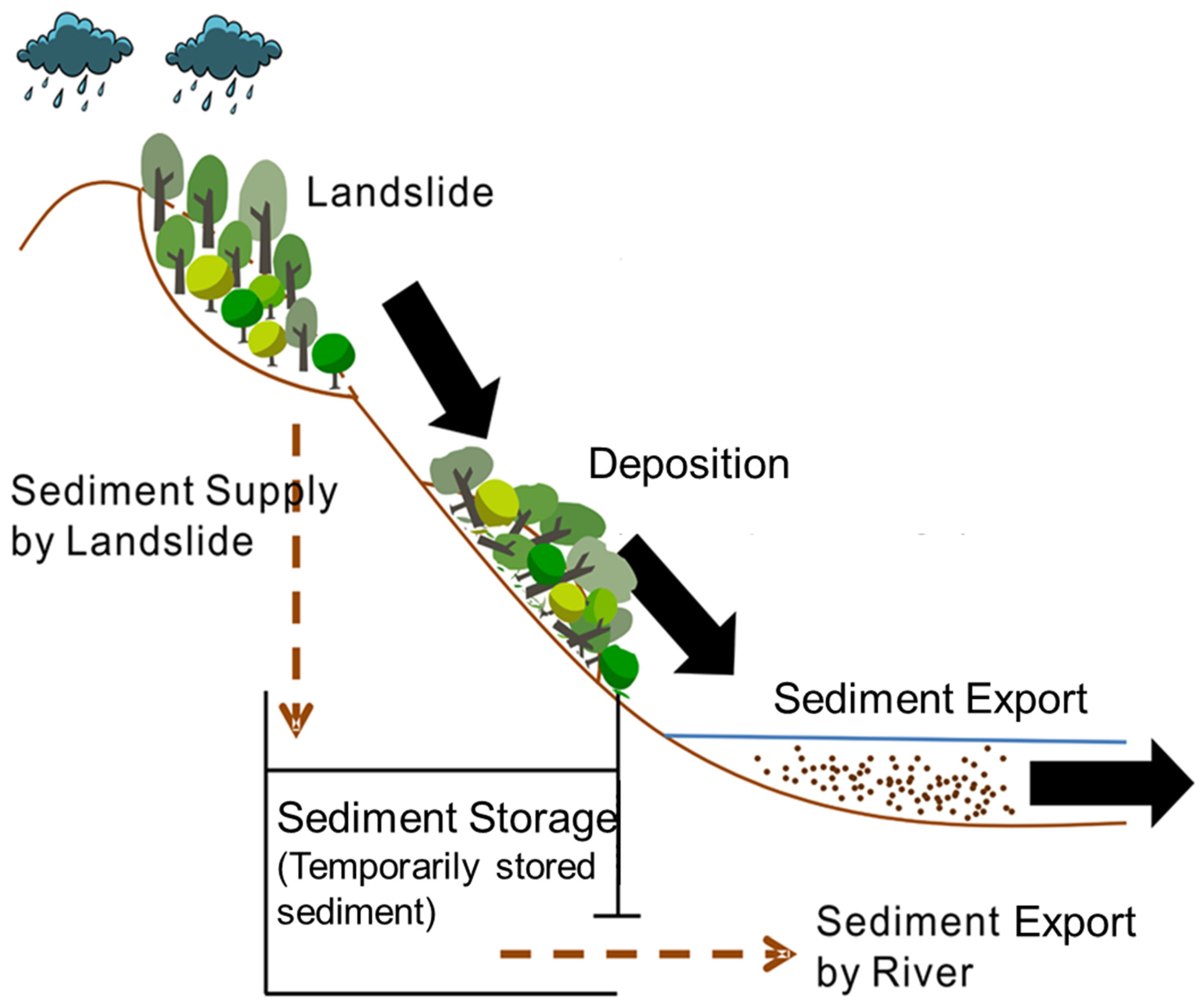
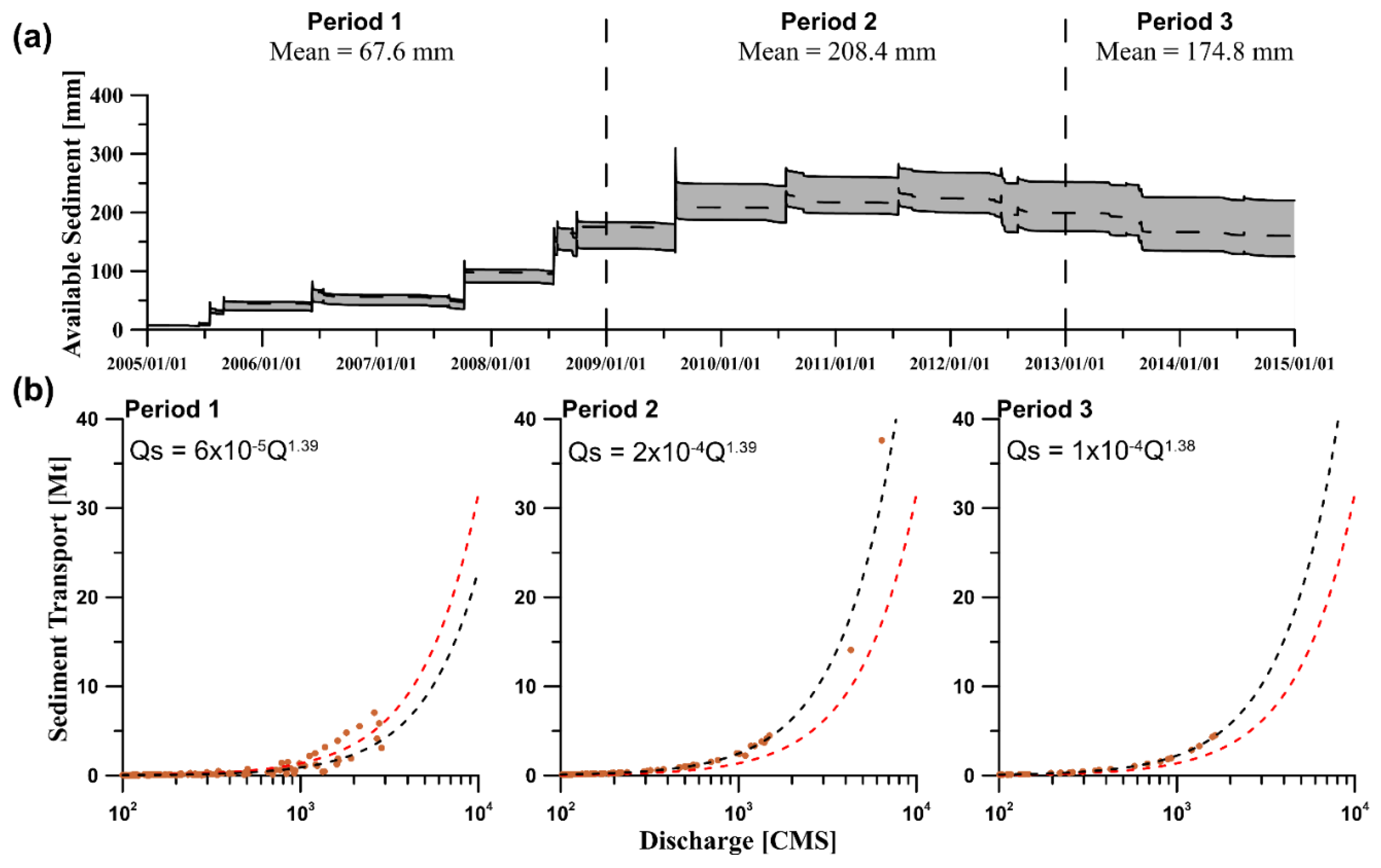
2.1.3. Sediment Storage

The amount of sediment storage is modulated by the input from landslide at time i (Sin,i) and the output through river at time i − 1 (Sout,i−1), which can be expressed by Equation (9).
S i = S i 1 S o u t , i 1 + S i n , i
Sin is derived from landslide volume estimation (Equations (6) and (7) in the unit of km3) and Sout is derived from fluvial sediment export calculation (Equation (8) in the unit of ton day−1). Sin and Sout should have identical unit before implementing Equation (9). Therefore, Sin is calculated by dividing the summation of Equations (6) and (7) by the watershed area (Area (km2) in Equation (10)) and the unit is converted to mm. Sin,i is the sediment contributing to sediment storage from landslides at time i in the condition of rainfall larger than 200 (mm), as shown in Equation (10). In Equation (9), the initial value of sediment storage, S0, is determined as the landslide volume after typhoon Mindulle in 2004, which is the first influential typhoon after 2001.
S i n , i = V i , n e w + V i , r e A r e a × 10 6
On the other hand, the amount of fluvial sediment export at time i, Sout,i (mm), can be calculated by cumulative volume of exported sediment during the time interval [0,T] (days) (Equation (11)). In Equation (11), D is sediment density ranging between 1.6–2.5 (ton m−3) (unpublished data).
S o u t , i = t = 0 T Q s , i , t d t D × A r e a × 10 3

2.1.4. Calibration of Landslide and Sediment Transport Model
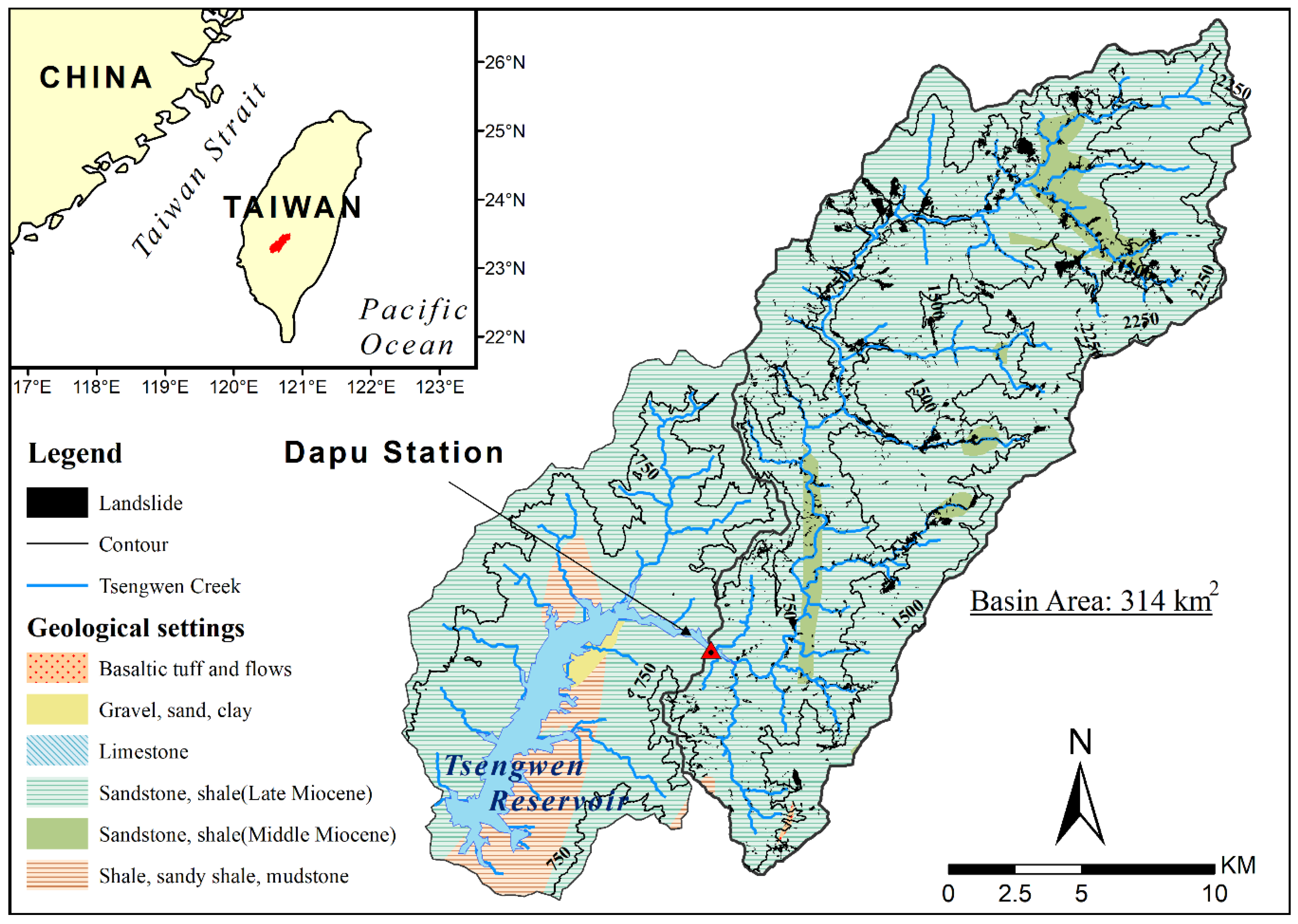
The integrated model proposed in this study is designed to simulate time-series of total landslide area (and thus volume) and sediment export on a daily basis. The observed data of total landslide area and event-based sediment export in 2005–2014 were used to estimate the parameters by simultaneously calibrating the two models. Over 100,000 parameter sets were generated by the uniform distribution in fixed ranges for each parameter (aLA: 0.6–0.8; bLA: 0.3–0.5; cLA: 3–5; aSC: 0.1–0.3; bSC: 0.7–0.9; cSC: 0.3–0.5; C: 0.8–1). Nash-Sutcliffe efficiency coefficient (EC) was used as the performance measure for landslide model. The value of EC ranges from negative infinity to 1.0 which represents perfect simulation. Nash-Sutcliffe efficiency coefficient with logarithmic value (EClog) was used for sediment transport model to assure the simulation for the low values which is overlooked by EC. The non-inferior solutions, based on EC and EClog for the two models, were selected by Pareto front [29]. As a result, with the help of this integrated model, one can obtain time-series simulated landslide volume and fluvial sediment export by only inputting the daily rainfall and river runoff.

2.2. Study Area

The study watershed is in the upstream of the Tsengwen Reservoir in southwestern Taiwan, with the Dapu gauging station as the watershed outlet (Figure 2). Tsengwen Creek drains a watershed of 314 (km2), which originates from the Ali Mountain. The watershed elevation ranges from 126 to 2609 m a.s.l., and the average slope is 26.1°. The land use type of Tsengwen Reservoir watershed is mostly composed of forest and agriculture, which accounts for 86% and 8%, respectively. The average annual rainfall in the study period (2005–2015) was around 3516 (mm) and 78% of the annual rainfall occur in wet season (June to October). Geological setting mainly comprises the alternation of sandstone and shale, making the Tsengwen Reservoir watershed highly erodible. The average landslide ratio in the study period is ~1.1%, ranging from 0.4–3.3%.
Given the conditions of frequent typhoons, highly erodible geology, high relief and steep gradient, Taiwan is featured by extremely high sediment production rates [30,31] and one of the most applicable places to landslide and sediment issues. Of which, reservoir siltation is one of the most serious problems to the reservoir management, particularly after Typhoon Morakot bringing a record-breaking rainfall in 2009. More than 3500 (mm) rainfall poured down in 5 days, resulting in more than 700 landslides and a 14% reduction in the reservoir capacity. The amount of siltation is equal to the total amount accumulated over the past 35 years.

2.3. Landslide Data

The yearly landslide maps taken by Formosa-2 (FS-2) are available on the website (http://246gis.swcb.gov.tw) provided by Soil and Water Conservation Bureau, Taiwan. Those maps reveal the landslide inventory for every year, which basically represent the collective impact from typhoons in a year. The FS-2 was launched and placed in a daily revisiting orbit in 2004. It was equipped with a high-spatial-resolution sensor providing panchromatic images at the resolution of 2 m and multispectral band images at 8 m. Therefore, FS-2 potentially can provide daily time-series satellite images that are capable of showing the instantaneous changes of land surfaces, e.g., the evolution of landslide after typhoon events. The image processing procedures and quality control regarding landslide delineation can be referred to Liu [32] for details. The following is a brief introduction to it. First, the raw FS-2 images are preprocessed automatically by the “Formosat-2 image processing system” (F2 AIPS), including band-to-band coregistration, orthorectification and geometrical registration of multi-temporal imagery. Second, each landslide patch was identified by integrating the Getis statistic, spectral index, and unsupervised K-means classification analysis [33]. The overall accuracy of automatically delineated landslide area can achieve 99.04% compared to those manually processed ones. It should be noted that the yearly landslide map of the study watershed was a compilation of several satellite images taken on adjacent dates to minimize cloud cover effects. After examining the date of a used image on a map, it is assumed that the landslide inventory in that year (e.g., at time i) is attributed to the preceding maximal rainfall event occurring after the date of image in the previous year (i.e., at time i − 1). There are 8 typhoon events and 2 rainstorm events shown in Table 1.

2.4. Hydrometric Data and Calculation of Sediment Transport

Long-term sediment concentration and runoff data (1957–2014) were derived from Hydrotech Research Institute, National Taiwan University and Tainan Hydraulics Laboratory, National Cheng Kung University. Of which, event-based sediment samples were taken every 1 to 3 h at Dapu gauging station during 9 rainstorm events (Table 2). Depth integrated water samples were obtained using a vertically mounted 1 L bottle attached to a weighted metal frame that was gradually lowered from the bridge. The US Geological Survey DH-48 sampler was not used because of its difficulty in sinking in turbulent flows > 2.5 (m s−1). Total suspended matter (TSM) was determined gravimetrically using pre-combusted 0.7 (μm) pore size GF/F filters [34]. The measured sediment concentration varied from 1331 to 68,197 (mg L−1). The highest measurement occurred when typhoon Morakot invaded. Hourly river runoff was also measured at Dapu station, which is maintained by Water Resources Agency, Ministry of Economic Affairs, Taiwan. The average runoff of the study period was around 48 (m3 s−1), but the daily runoff fluctuated from ~0.1 to 6815 (m3 s−1). Typhoon Morakot led to an observed maximal runoff on 9 August 2009.
Flux estimator is essential in this study to calculate sediment export during a rainstorm event given the conditions of discrete sediment concentration measurement and continuous river runoff data. The rating curve method is one of the most appropriate flux estimation methods and has been widely applied to rivers in Taiwan, particularly suitable for the sediment flux estimation [13,17]. This method presumes that a power function (i.e., F = aQb) exists between the observed runoff (Q) and sediment flux (F) that is the product of observed sediment concentration and the instantaneous river runoff. The coefficients of the power function, a and b, can be derived from the observed sediment fluxes and the river runoff by the log-linear least-square method [17]. For the non-typhoon periods, the rating curve, constructed by the long-term sediment concentration and runoff data, was used to calculate daily sediment export by substituting daily runoff into the rating curve (i.e., F(g s−1) = 33.94Q2.90, R2 = 0.84). Moreover, 9 event-based rating curves were established for each individual rainstorm event. Each rating curve was then applied to hourly runoff during the event to calculate hourly sediment export. The summation of the hourly sediment export was the total sediment being flushed off the watershed in the event. Besides, it is well known that the rating curve method inherently underestimates the summation of the sampled sediment export within a concerned period, particularly for the fluxes at the highest runoff. Therefore, a bias-correction factor proposed by Kao et al. [17] was introduced to reduce residuals.

3. Results

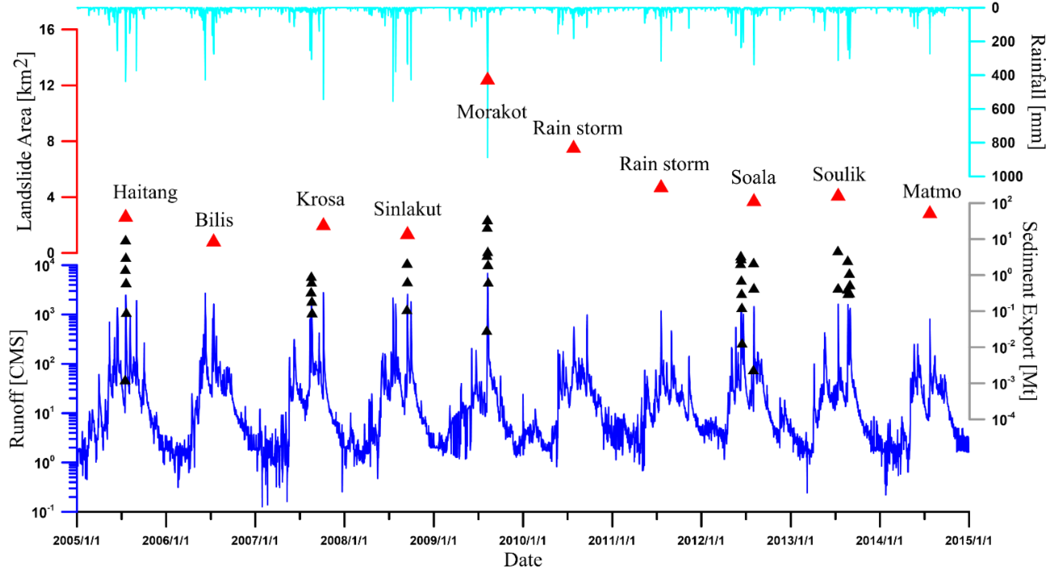
3.1. Observed Total Landslide Area and Sediment Export in Tsengwen Reservoir Watershed

Figure 3 illustrates the observations in this study, including daily rainfall, river runoff, sampled sediment data, and yearly total landslide area (named after the 8 typhoon and 2 rainstorm events). Among the events, the observed minimum daily rainfall and runoff occurred during the 2010 rainstorm, which were 183 (mm day−1) and 979 (m3 s−1), respectively, while the highest daily rainfall and runoff reached 878 (mm day−1) and 6815 (m3 s−1) during typhoon Morakot in 2009 (Table 1). As for observed total landslide area, before typhoon Morakot on 9/8/2009, the total landslide area ranged between ~1 to ~3 (km2). The maximum area, 12.53 (km2), was triggered by typhoon Morakot. Afterwards, the landslide area gradually decreased from ~12 (km2) to ~2 (km2). However, the smallest total landslide area was found after typhoon Bilis rather than the smallest rainfall event, i.e., the 2010 rainstorm. Typhoon Bilis had the 5th highest daily rainfall, 427 (mm day−1), but resulted in merely 0.94 (km2) landslide area. Poor rainfall–landslide area relationship (r = 0.38) in Tsengwen Reservoir watershed hampers the application of the conventional regression models [19,26].
Table 2 shows the sediment export during the 9 sampled rainfall events. Maximum sampled sediment concentration and runoff were 68.20 (g L−1) and 5797 (m3 s−1), respectively, during Typhoon Morakot. Event-based rating curved were established for each individual event to estimate sediment export, and the R2 ranged from 0.83–0.99. Therefore, sediment export of the 9 sampled rainfall events fell between 2.03–67.57 (Mt).

3.2. Calibration of Model Parameters

The landslide model and the sediment transport model were calibrated simultaneously but were evaluated by different performance measures, i.e., EC and EClog, respectively. Figure 4 illustrates the Pareto front of EC against EClog with the 23 red dots representing the non-inferior parameter sets (out of the 100,000 parameter sets). The values of the calibrated parameters are shown in Table 3 with the shaded ones representing its p-value less than 0.05. The EC values of the 23 parameter sets are between 0.87–0.89 for the landslide model, and EClog are between 0.86–0.91 for the sediment transport model.
For the landslide model, the landslide reactivated ratio, a L A , is between 0.68–0.74 among the 23 parameter sets, which means that more than half of the previous total landslide area would be retriggered. Representing new landslide, the parameter b L A and c L A are between 0.30–0.50 and 3.19–3.92, respectively. As for the sediment transport model, the intercept, a S C , and slope, c S C , in rating curve are 0.10–0.24 and 0.30–0.42. The scaling parameter for sediment storage, b S C , is between 0.70–0.80. The contributing ratio, C, is between 0.81–1.00, indicating that the sediment production rate on reactivated landslide is nearly at the same order as the new landslide. Overall, the 4th parameter set is defined as the optimal one because 6 out of 7 parameters are identified as significant and parameter C is not as sensitive as the other parameters (see Section 4.2). The optimal parameters are aLA = 0.72, bLA = 0.39, cLA = 3.62, aSC = 0.15, bSC = 0.71, cSC = 0.36 and C = 0.86, and the EC and EClog are 0.89 and 0.90, respectively.

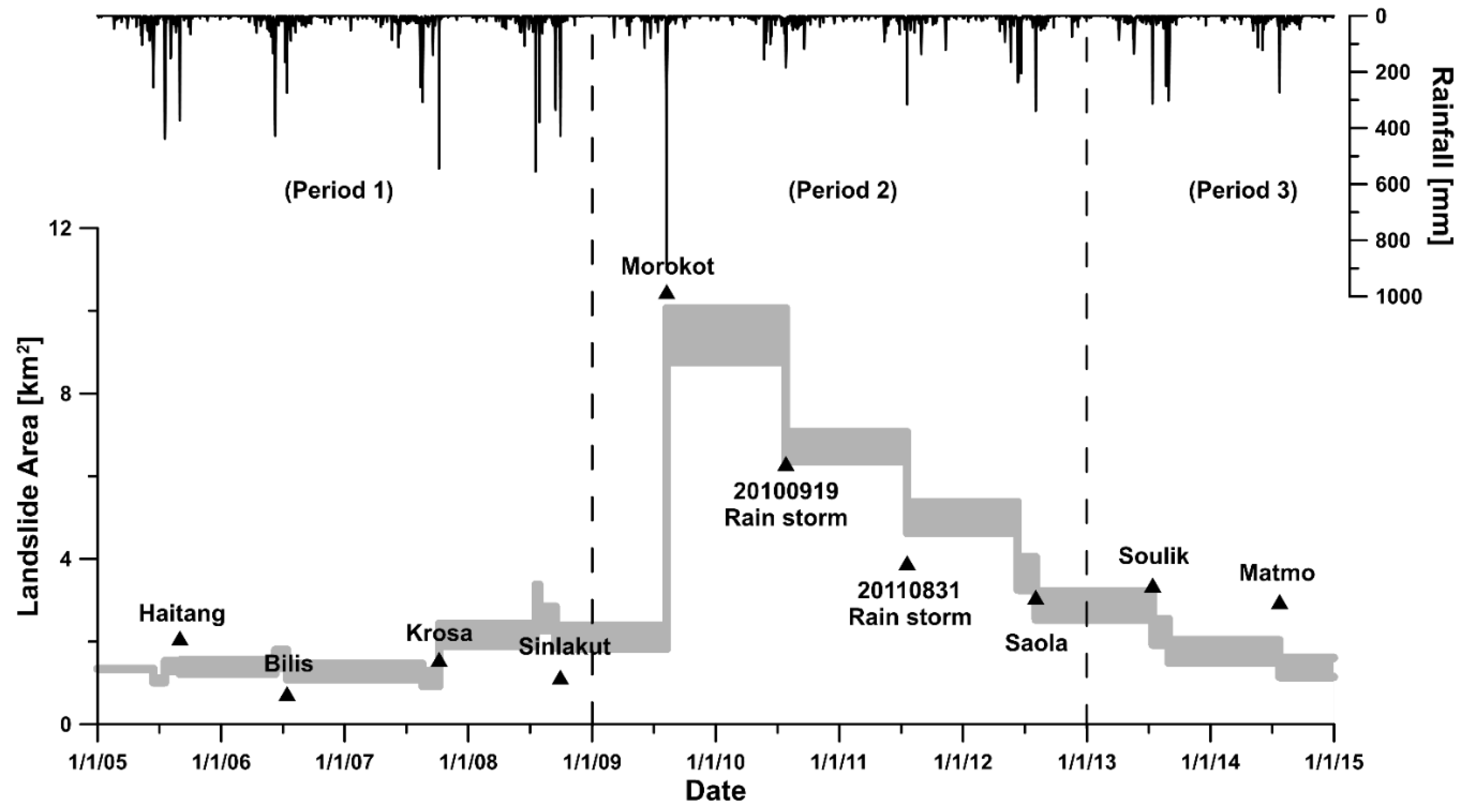
3.3. Simulated Time-Series Total Landslide Area

The simulated time-series total landslide area is shown in Figure 5. The gray zone in Figure 5 embraced the simulations from the 23 parameter sets. In the landslide model, landslide was triggered only when daily rainfall exceeded the designate threshold, i.e., 200 (mm day−1). Without considering the recovery of landslide scars, the simulated total landslide area remained a constant before the new landslide generated, resulting in the stepwise curve of simulated landslide area. During the period of 1/1/2005–31/12/2008 (Period 1), the simulated total landslide area was between 1–4 (km2) while the observed total landslide area was between 1–3 (km2). During Period 2 (1/1/2009–31/12/2012) with the invasion of typhoon Morakot, the simulated total landslide area ranged from ~10 to 3 (km2). After typhoon Morakot, the total landslide model well simulated the decreasing trend of total landslide area. However, it slightly overestimated the total landslide area triggered by 9/9/2010 and 31/8/2011 rainstorm events. During the Period 3 (1/1/2013–31/12/2014), the simulated total landslide area gradually decreased from 2 (km2) to 1 (km2), which was close to the level before typhoon Morakot.

3.4. Simulated Sediment Export

Figure 6a illustrates the simulated time-series sediment export (gray line) as well as the observed one (black triangles). The daily sediment export varied at 7-order of magnitude (~10−4–~101 (Mt)), revealing the flushing nature of Taiwan rivers. The low-end values of sediment export shifted from ~10−5 (Mt) in Period 1 to ~10−3 (Mt) in Period 2, and then to ~10−4 (Mt) in Period 3. The sediment transport model simulated the observed sediment export well with EClog = 0.90 (Figure 6b). The error bars in Figure 6b represent the 2-fold standard deviation of the simulated ranges among the 23 non-inferior parameter sets. To illustrate the changes of carrying capacity of the river, the simulated daily sediment export was normalized by daily river runoff (i.e., sediment export/runoff, Figure 6c). It is found that the carrying capacity was at the lowest in Period 1 (mean = 0.003 t m−3), and it increased to the highest in Period 2 (0.006 t m−3), and then decreased to a middle value in Period 3 (0.005 t m−3). It indicates that one unit river runoff could deliver more sediment during the post-Morakot period, owing to more sediment storage.

4. Discussion

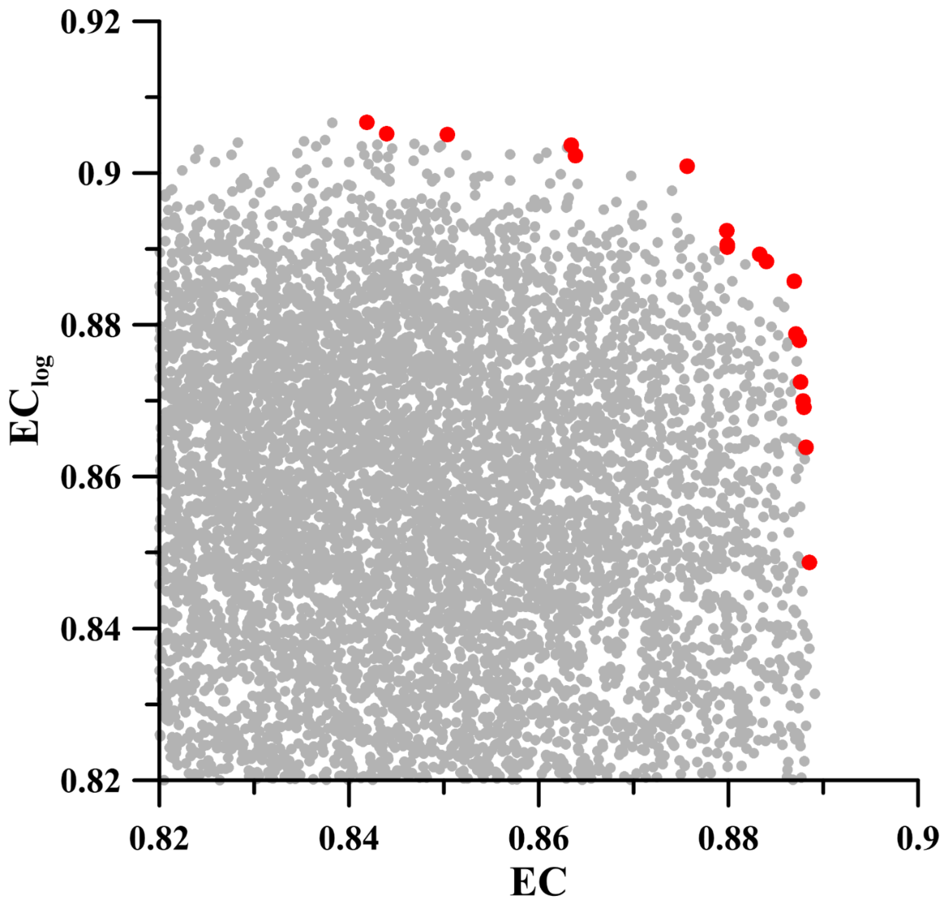
4.1. Best-Fit Parameter Sets

The 23 non-inferior parameter sets derived from the Pareto front were determined as the best-fit parameter values (Table 3). The reactivated ratio ( a L A ), ranging between 0.68–0.74, is close to the upper range of the observed reactivated ratio (Table 1). Previous studies have addressed the reactivated ratio for watersheds in Taiwan, showing values between 0.40–0.93 in Chenyoulan watershed in central Taiwan [25], and 0.52–0.67 in Sinwulu and Luye watersheds in Eastern Taiwan [35]. It can be concluded that more than half of the total landslide area would be retriggered in Taiwan watersheds where typhoons disturb recurrently every year.
The rating curve intercept parameter (Equation (8)), which is the product of asc and ( S i S m e a n ) b s c , ranges from 0.12–4.35 and is compared with the intercept in the conventional rating curve, i.e., a in the equation of aQb. The intercept derived in this study is much higher than that of other world rivers, ranging from 0.01–0.04 [36], which indicates that there is considerable sediment being transported during low-to-medium flow period. In other words, in conditions of small rainfall events, the river in this study has sufficient sediment storage to support higher sediment export in comparison with other rivers in the world. Correspondingly, it is essential to consider sediment storage in the model. As for the rating curve slope, parameter cSC, between 1.3–1.42, agrees with the results of 16 primary rivers in Taiwan (ranging mostly from 1 to 2.5) [17]. The values of slope parameter for rivers worldwide also fall within 1 to 2 [36].
The parameter C (in Equation (7)) ranging from 0.81–1.00 means that the average landslide depth (or erosion rate) for the reactivated landslide is nearly 1.4–1.7 (m). Tsai et al. [37] investigated the erosion rate on 13 reactivated landslides in Shimen Reservoir watershed in north Taiwan and obtained the erosion rate at 0.78–1.06 (m year−1) which was shallower than that of our study watershed, perhaps owing to different geological conditions. The geology of Shimen Reservoir watershed comprises mainly schist and phyllite, while Tsengwen Reservoir watershed consists of more erodible alternations of sandstone and shale (Figure 2).

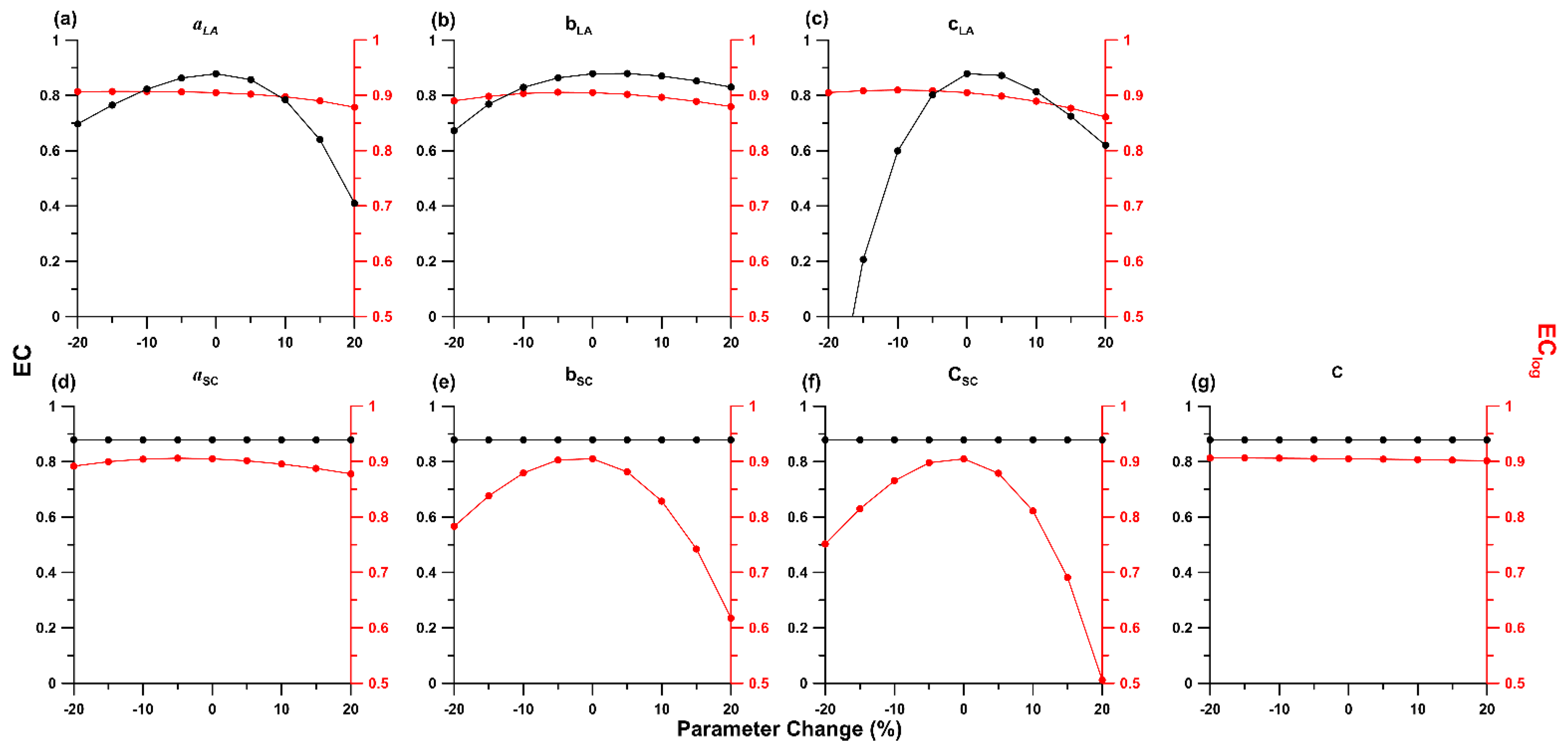
4.2. Sensitivity Analysis

To understand the model responses to the change of each parameter, the sensitivity analysis is presented here. The sensitivity analysis was implemented via adjusting one of the parameters in the optimal parameter set from −20% to +20% while leaving the rest parameters unchanged, to examine model responses to each respective parameter changes (Figure 7). The model responses are presented by the changes of EC and EClog.
Figure 7 illustrates the results of sensitivity analysis for the landslide model (Figure 7a–c) and the sediment transport model (Figure 7d–g). The landslide model is most sensitive to the adjustments (+/- 20% of the optimal value) of aLA and cLA (black circle in Figure 7a,c), resulting in −55%/−21% and −33%/−100% changes, respectively, on the EC of the landslide model. The model is less sensitive to parameter bLA, while the EC varies within −25% of the optimal one, i.e., 0.89. The sediment transport model is relatively insensitive to the landslide model parameters. The adjustments would lower the EClog to 0.86 (i.e., −4.4%) at most.
The results from landslide model are the inputs of the sediment transport model. The four parameters (Figure 7d–g) are irrelevant to the landslide model; hence the black line remains unchanged. The most sensitive parameters to the sediment transport model (red circle) are the slope parameter, cSC of the rating curve, with the EClog decreasing to 0.75 (−16%) and to 0.51 (−43%) from 0.90, respectively, in respond to the −20% and 20% adjustments of the optimal value. The parameter bsc that regulates the effect of sediment storage on sediment export is sensitive as well, with the EClog deceasing to 0.78 (−13%)/0.62 (-31%) for the −20%/+20% adjustments.

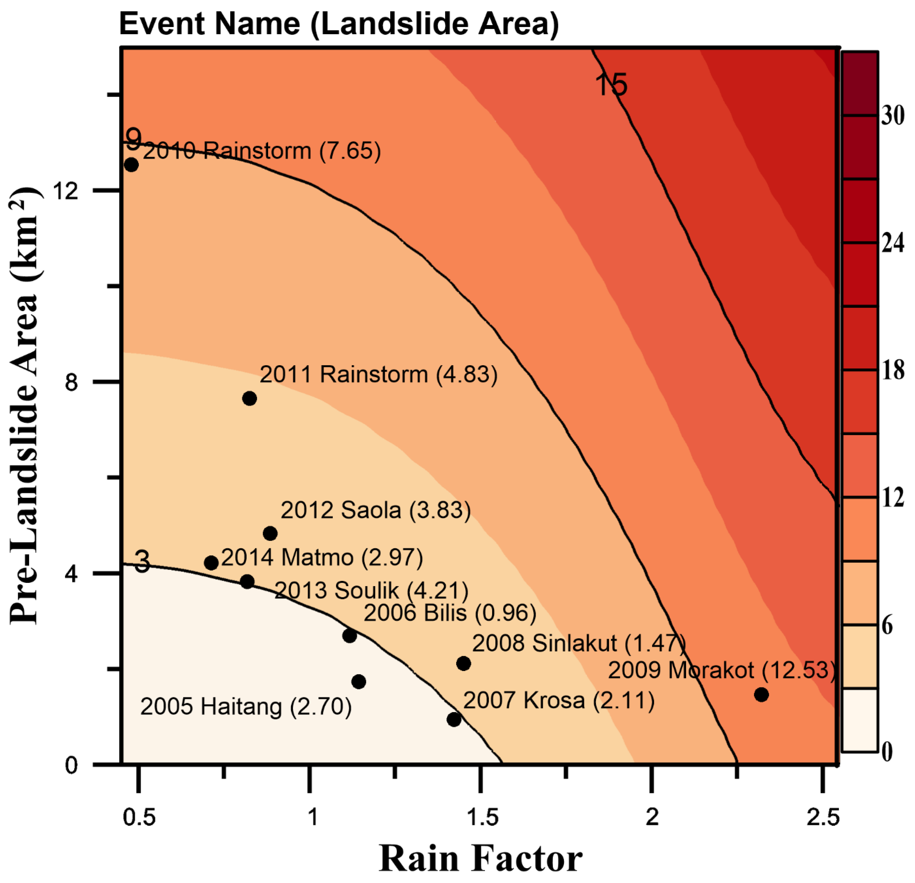
4.3. The Controlling Factors of Total Landslide Area

Figure 8 illustrates a contour diagram of the estimated total landslide area as a function of rain factor (the x-axis, i.e., R/R* in Equation (5)) and pre-landslide area (the y-axis, total landslide area in the previous year). The estimated total landslide area was estimated by substituting the optimal parameter sets in the landslide model (Equation (6)). At a given pre-landslide area, higher rainfall would trigger larger total landslide area, particularly when rain factor is larger than 1.5. When a fixed rain factor is given, the total landslide area is positively correlated to the one in the previous year. However, the correlation becomes weaker when rain factor gets larger. Overall, it indicates that pre-landslide area controls the total landslide area when rainfall is small, like the cases in 2010–2013. Rainfall controls the total landslide area when rainfall is large, as seen in the cases in 2005–2008.
Rainfall is long regarded as the key factor to trigger landslide and is used as the only independent variable to estimate landslide area by many previous studies [19,26]. We suggest that in landslide-dominated region considering not only the rainfall but also previous landslide status as controlling factors in simulating total landslide area is necessary.

4.4. The Sediment Storage and Controlling Factors of Sediment Export

The best-fit parameter sets (in Table 3) were used to estimate a range of sediment storage as the gray zone in Figure 9a. It shows that the study period (1/1/2005–31/12/2014) was divided into three periods (i.e., Period 1, Period 2, and Period 3 as mentioned in Section 3.3) to clearly explain the effects of sediment storage on sediment export. The sediment storage ranged from 0–150 (mm) in Period 1 and suddenly increased to as much as 250 (mm) in Period 2, and then gradually decreased to ~100 (mm) in Period 3. The range of estimated sediment storage became large in Period 2 and Period 3, indicating the relatively uncertain estimation of the available sediment after the extreme weather event, i.e., typhoon Morakot. The ranges of the sediment storage also reflect the uncertain estimation of the total landslide area (Figure 5).
Figure 9b illustrates the rating curve of the simulated sediment export against river runoff for the three periods. The exponents of the three rating curves remain at ~1.38–1.39, indicating the similar effect of stream power on sediment export. However, the coefficients of the rating curves vary among the three periods. At a given river runoff, Period 2 would have the highest sediment export, and then Period 3 and Period 1 would have the lowest. The coefficient in the rating curve reflects the sediment supply in the watershed. The coefficients for Period 2 (i.e., 2 × 10⁻⁴) and Period 3 (1 × 10⁻⁴) are one-order of magnitude larger than Period 1 (6 × 10⁻⁵), indicating substantial sediment supply after typhoon Morakot (Figure 6c). The impact of residual sediment was also found in Choshui watershed in central Taiwan after a severe landslide event (i.e., ChiChi earthquake in 1999), which can last for ~6 years [20]. The recession time is comparable to the Morakot case in this study. We believed that the model with the idea of sediment storage can refine the simulation of sediment export in a more validated way.
Sediment transfer, from hillslope to channel and off watershed, is a global issue wherever there is soil erosion, particularly crucial in the landslide-prone region. Sediment deposition will lead to flood plain and channel aggradation and further result in water level rise and sediment-related hazards. The estimation of sediment storage might help to understand the relevant risk. Period 3 in this study is prone to the risk compared to Period 1 owing to more readily-eroded sediment in the hillslope and channel in Period 3. Moreover, landscape evolution can be inferred from watershed-wide erosion rate [1,2]. However, discrepancy exists between the rates inferred from landslide volume (e.g., digital elevation models (DEMs) derived from photogrammetry of aerial photographs) and fluvial sediment export [38]. The sediment storage might help to explain the discrepancy and prolonged/delayed response of sediment transport to landslide [39,40,41]. Zhang et al. [42] demonstrated that intense monsoonal runoff drove sediment transfer and depositional processes until 2 years after the Wenchuan earthquake, implying the applicability of the sediment storage concept (if earthquake-induced landslide model was incorporated). The sediment storage could also help to explain sediment transport is transport-limited or supply-limited [43].

5. Conclusions

Linkage between sediment supply from landslides and export by fluvial system is unclear due to insufficient knowledge about the spatial and temporal pattern of the sediment deposition within the watersheds, especially in landslide-dominated regions, where highly frequent occurrence of landslide affirms the effect of sediment storage not to be ignored. In this study, we established a conceptual model that simulates the chain reaction from rainfall, landslide to sediment export by considering the effects of pre-landslide area and the sediment storage. Rainfall at a higher resolution temporal scale (e.g., hours) could strongly modulate the timing landslide debris reach the rivers from the slopes, affecting both landslide (e.g., depth of the failure surface; velocity; movement typologies; run-out distance) and water erosion (either splash, sheet, rill, or gully erosion) processes. Nevertheless, the sediment storage variable, to some extent, cleverly and implicitly considers the complexity of temporal and spatial distribution of sediment.
In our landslide model, the excellent performance, EC = 0.89, indicates that the incorporation of the reactivated landslide is crucial in the landslide-dominated region like Taiwan who faces 3–5 typhoon invasions every year. The reactivation of previous landslides significantly contributes available sediment as much as the new landslides. However, the reactivation ratio can be improved and should vary among landslide occurrences, seasons, and even among topographic conditions. As for the sediment transport model, it is found that higher sediment storage after substantial landslide input induced by catastrophic typhoon events could elevate sediment export 1-order of magnitude higher than that before the input. Several studies have indicated the effects of temporarily stored sediment on sediment export from the observed C-Q relation [13,19,20]. In this study, we further quantify the amount of sediment storage and its consequent effects. Furthermore, we suggest that the concept of storage could be applied to other stock relevant issues, such as the lingering effects of litter fall on nutrient release, to quantify the effects on biogeochemical cycle [44]. However, bedload transport is one of the limitations in this study, which can be improved by incorporating bedload transportation estimation equations in the model [45,46]. Nevertheless, the validation of bedload transport is always a problem in the field [47].
Global warming is proven in the ascendant and is resulting in more unprecedented weather extremes. The increased rainfall intensity has led to magnified sediment export from Taiwan rivers [13,26]. Our proposed model could benefit the understanding of the sediment dynamics in the watersheds. Pre-landslide area and the current sediment storage are both crucial in controlling sediment budget in the river.

Author Contributions

Data curation, T.-Y.T.; formal analysis, T.-Y.T. and T.-Y.L.; funding acquisition, J.-C.H.; methodology, J.-C.H.; project administration, J.-C.H.; resources, Y.-C.C., M.-Y.J. and C.-C.L.; supervision, J.-C.H. and T.-Y.L.; Visualization, T.-Y.T.; writing—original draft, T.-Y.T.; writing—review & editing, T.-Y.L. All authors have read and agreed to the published version of the manuscript.

Funding

This research was funded by [Taiwan Ministry of Science and Technology] grant number [NSC 102-2923-M-002 -001-MY3, MOST 107-2621-B-002-003-MY3, MOST 106-2116-M-002-020], [Austrian Science Fund] grant number [FWF I 1396-B16], and [NTU Research Center for Future Earth] grant number [107L901004].

Acknowledgments

We thank Hydrotech Research Institute, National Taiwan University and Tainan Hydraulics Laboratory, National Cheng Kung University for providing sediment concentration and discharge data, and Water Resources Agency, Ministry of Economic Affairs for providing hourly discharge data.

Conflicts of Interest

The authors declare no conflict of interest.

References

  1. Dadson, S.; Hovius, N.; Chen, H.; Dade, W.B.; Hsieh, M.-L.; Willett, S.D.; Hu, J.-C.; Horng, M.-J.; Chen, M.-C.; Stark, C.P.; et al. Links between erosion, runoff variability and seismicity in the Taiwan orogen. Nat. Cell Biol. 2003, 426, 648–651. [Google Scholar] [CrossRef]
  2. Schmidt, J.C.; Parnell, R.A.; Grams, P.E.; Hazel, J.E.; Kaplinski, M.A.; Stevens, L.E.; Hoffnagle, T.L. The 1996 controlled flood in Grand Canyon: Flow, sediment transport, and geomorphic change. Ecol. Appl. 2001, 11, 657–671. [Google Scholar] [CrossRef]
  3. West, A.J.; Galy, A.; Bickle, M. Tectonic and climatic controls on silicate weathering. Earth Planet. Sci. Lett. 2005, 235, 211–228. [Google Scholar] [CrossRef]
  4. Neil, D.T.; Orpin, A.R.; Ridd, P.V.; Yu, B. Sediment yield and impacts from river catchments to the Great Barrier Reef lagoon: A review. Mar. Freshw. Res. 2002, 53, 733–752. [Google Scholar] [CrossRef]
  5. Rabalais, N.N.; Turner, R.E.; Gupta, B.K.S.; Platon, E.; Parsons, M.L. Sediments Tell the History of Eutrophication and Hypoxia in the Northern Gulf of Mexico. Ecol. Appl. 2007, 17, S129–S143. [Google Scholar] [CrossRef]
  6. Hilton, R.G.; Galy, A.; Hovius, N.; Horng, M.-J.; Chen, H. The isotopic composition of particulate organic carbon in mountain rivers of Taiwan. Geochim. Cosmochim. Acta 2010, 74, 3164–3181. [Google Scholar] [CrossRef] [Green Version]
  7. Kao, S.-J.; Shiah, F.-K.; Wang, C.-H.; Liu, K.-K. Efficient trapping of organic carbon in sediments on the continental margin with high fluvial sediment input off southwestern Taiwan. Cont. Shelf Res. 2006, 26, 2520–2537. [Google Scholar] [CrossRef]
  8. Galy, V.; France-Lanord, C.; Lartiges, B. Loading and fate of particulate organic carbon from the Himalaya to the Ganga–Brahmaputra delta. Geochim. Cosmochim. Acta 2008, 72, 1767–1787. [Google Scholar] [CrossRef]
  9. Hilton, R.G.; Galy, A.; Hovius, N.; Chen, M.-C.; Horng, M.-J.; Chen, H. Tropical-cyclone-driven erosion of the terrestrial biosphere from mountains. Nat. Geosci. 2008, 1, 759–762. [Google Scholar] [CrossRef] [Green Version]
  10. Hilton, R.G.; Galy, A.; Hovius, N.; Horng, M.-J.; Chen, H. Efficient transport of fossil organic carbon to the ocean by steep mountain rivers: An orogenic carbon sequestration mechanism. Geology 2011, 39, 71–74. [Google Scholar] [CrossRef] [Green Version]
  11. Kao, S.-J.; Liu, K.-K. Particulate organic carbon export from a subtropical mountainous river (Lanyang Hsi) in Taiwan. Limnol. Oceanogr. 1996, 41, 1749–1757. [Google Scholar] [CrossRef]
  12. Huang, J.-C.; Kao, S.-J.; Hsu, M.-L.; Lin, J.-C. Stochastic procedure to extract and to integrate landslide susceptibility maps: An example of mountainous watershed in Taiwan. Nat. Hazards Earth Syst. Sci. 2006, 6, 803–815. [Google Scholar] [CrossRef]
  13. Lee, T.-Y.; Huang, J.-C.; Lee, J.-Y.; Jien, S.-H.; Zehetner, F.; Kao, S.-J. Magnified Sediment Export of Small Mountainous Rivers in Taiwan: Chain Reactions from Increased Rainfall Intensity under Global Warming. PLoS ONE 2015, 10, e0138283. [Google Scholar] [CrossRef] [PubMed]
  14. Kao, S.J.; Huang, J.C.; Lee, T.Y.; Liu, C.C.; Walling, D.E. The changing rainfall–runoff dynamics and sediment response of small mountainous rivers in Taiwan under a warming climate. In Sediment Problems and Sediment Management in Asian River Basins; (IAHS Publ 349); IAHS Press: Wallingford, UK, 2011. [Google Scholar]
  15. Milliman, J.D.; Syvitski, J.P. Geomorphic/Tectonic Control of Sediment Discharge to the Ocean: The Importance of Small Mountainous Rivers. J. Geol. 1992, 100, 525–544. [Google Scholar] [CrossRef]
  16. Milliman, J.D.; Farnsworth, K.L. River Discharge to the Coastal Ocean: A Global Synthesis; Cambridge University Press: Cambridge, UK, 2013. [Google Scholar]
  17. Kao, S.-J.; Lee, T.-Y.; Milliman, J.D. Calculating Highly Fluctuated Suspended Sediment Fluxes from Mountainous Rivers in Taiwan. Terr. Atmos. Ocean. Sci. 2005, 16, 653. [Google Scholar] [CrossRef] [Green Version]
  18. Lee, T.-Y.; Huang, J.-C.; Kao, S.-J.; Tung, C.-P. Temporal variation of nitrate and phosphate transport in headwater catchments: The hydrological controls and land use alteration. Biogeosciences 2013, 10, 2617–2632. [Google Scholar] [CrossRef] [Green Version]
  19. Fuller, C.W.; Willett, S.D.; Hovius, N.; Slingerland, R. Erosion Rates for Taiwan Mountain Basins: New Determinations from Suspended Sediment Records and a Stochastic Model of Their Temporal Variation. J. Geol. 2003, 111, 71–87. [Google Scholar] [CrossRef] [Green Version]
  20. Milliman, J.D.; Lee, T.Y.; Huang, J.-C.; Kao, S.J. Temporal and spatial responses of river discharge to tectonic and climatic perturbations: Choshui River, Taiwan, and Typhoon Mindulle (2004). Proc. Int. Assoc. Hydrol. Sci. 2015, 367, 29–39. [Google Scholar] [CrossRef]
  21. Van Sickle, J.; Beschta, R.L. Supply-based models of suspended sediment transport in streams. Water Resour. Res. 1983, 19, 768–778. [Google Scholar] [CrossRef] [Green Version]
  22. Hovius, N.; Stark, C.P.; Allen, P.A. Sediment flux from a mountain belt derived by landslide mapping. Geology 1997, 25, 231–234. [Google Scholar] [CrossRef] [Green Version]
  23. Malamud, B.D.; Turcotte, D.L.; Guzzetti, F.; Reichenbach, P. Landslide inventories and their statistical properties. Earth Surf. Process. Landf. 2004, 29, 687–711. [Google Scholar] [CrossRef]
  24. Amos, K.J.; Alexander, J.; Horn, A.; Pocock, G.D.; Fielding, C.R. Supply limited sediment transport in a high-discharge event of the tropical Burdekin River, North Queensland, Australia. Sedimentology 2004, 51, 145–162. [Google Scholar] [CrossRef]
  25. Lin, G.-W.; Chen, H.; Chen, Y.-H.; Horng, M.-J. Influence of typhoons and earthquakes on rainfall-induced landslides and suspended sediments discharge. Eng. Geol. 2008, 97, 32–41. [Google Scholar] [CrossRef]
  26. Chen, Y.-C.; Chang, K.-T.; Chiu, Y.-J.; Lau, S.-M.; Lee, H.-Y. Quantifying rainfall controls on catchment-scale landslide erosion in Taiwan. Earth Surf. Process. Landf. 2013, 38, 372–382. [Google Scholar] [CrossRef]
  27. Aerial Survey Office, Taiwan Forestry Bureau. Report of Aerial Survey of Landslide in Tsengwen Reservoir Watershed; Management Bureau of Tsengwen Reservoir, Taiwan Press: Taipei, Taiwan, 1980. [Google Scholar]
  28. Turowski, J.M.; Rickenmann, D.; Dadson, S.J. The partitioning of the total sediment load of a river into suspended load and bedload: A review of empirical data. Sedimentology 2010, 57, 1126–1146. [Google Scholar] [CrossRef]
  29. Madsen, H. Automatic calibration of a conceptual rainfall–runoff model using multiple objectives. J. Hydrol. 2000, 235, 276–288. [Google Scholar] [CrossRef]
  30. Li, Y.-H. Denudation of Taiwan Island since the Pliocene Epoch. Geology 1976, 4, 105–108. [Google Scholar] [CrossRef]
  31. Milliman, J.D.; Meade, R.H. World-Wide Delivery of River Sediment to the Oceans. J. Geol. 1983, 91, 1–21. [Google Scholar] [CrossRef]
  32. Liu, C.-C. Processing of FORMOSAT-2 Daily Revisit Imagery for Site Surveillance. IEEE Trans. Geosci. Remote Sens. 2006, 44, 3206–3214. [Google Scholar] [CrossRef]
  33. Liu, C.-C.; Shieh, C.-L.; Lin, J.-C.; Wu, A.-M. Classification of non-vegetated areas using Formosat-2 high spatiotemporal imagery: The case of Tseng-Wen Reservoir catchment area (Taiwan). Int. J. Remote Sens. 2011, 32, 8519–8540. [Google Scholar] [CrossRef]
  34. Milliman, J.D.; Lin, S.-W.; Kao, S.-J.; Liu, J.-P.; Liu, C.-S.; Chiu, J.-K.; Lin, Y.-C. Short-term changes in seafloor character due to flood-derived hyperpycnal discharge: Typhoon Mindulle, Taiwan, July 2004. Geology 2007, 35, 779. [Google Scholar] [CrossRef] [Green Version]
  35. Chen, H.; Lin, G.-W.; Lu, M.-H.; Shih, T.-Y.; Horng, M.-J.; Wu, S.-J.; Chuang, B. Effects of topography, lithology, rainfall and earthquake on landslide and sediment discharge in mountain catchments of southeastern Taiwan. Geomorphology 2011, 133, 132–142. [Google Scholar] [CrossRef]
  36. Asselman, N. Fitting and interpretation of sediment rating curves. J. Hydrol. 2000, 234, 228–248. [Google Scholar] [CrossRef]
  37. Tsai, Z.-X.; You, G.J.-Y.; Lee, H.-Y.; Chiu, Y.-J. Use of a total station to monitor post-failure sediment yields in landslide sites of the Shihmen reservoir watershed, Taiwan. Geomorphology 2012, 139, 438–451. [Google Scholar] [CrossRef]
  38. Clapuyt, F.; Vanacker, V.; Christl, M.; Van Oost, K.; Schlunegger, F. Spatio-temporal dynamics of sediment transfer systems in landslide-prone Alpine catchments. Solid Earth 2019, 10, 1489–1503. [Google Scholar] [CrossRef] [Green Version]
  39. Koi, T.; Hotta, N.; Ishigaki, I.; Matuzaki, N.; Uchiyama, Y.; Suzuki, M. Prolonged impact of earthquake-induced landslides on sediment yield in a mountain watershed: The Tanzawa region, Japan. Geomorphology 2008, 101, 692–702. [Google Scholar] [CrossRef]
  40. Hovius, N.; Meunier, P.; Lin, C.-W.; Chen, H.; Chen, Y.-G.; Dadson, S.; Horng, M.-J.; Lines, M. Prolonged seismically induced erosion and the mass balance of a large earthquake. Earth Planet. Sci. Lett. 2011, 304, 347–355. [Google Scholar] [CrossRef]
  41. Chen, Y.-C.; Wu, Y.-H.; Shen, C.-W.; Chiu, Y.-J. Dynamic Modeling of Sediment Budget in Shihmen Reservoir Watershed in Taiwan. Water 2018, 10, 1808. [Google Scholar] [CrossRef] [Green Version]
  42. Zhang, F.; Jin, Z.; West, A.J.; An, Z.; Hilton, R.G.; Wang, J.; Li, G.; Densmore, A.L.; Yu, J.; Qiang, X.; et al. Monsoonal control on a delayed response of sedimentation to the 2008 Wenchuan earthquake. Sci. Adv. 2019, 5, eaav7110. [Google Scholar] [CrossRef] [Green Version]
  43. Lisle, T.E.; Church, M. Sediment transport-storage relations for degrading, gravel bed channels. Water Resour. Res. 2002, 38, 1-1-1-14. [Google Scholar] [CrossRef]
  44. Chang, C.-T.; Wang, L.-J.; Huang, J.-C.; Liu, C.-P.; Wang, C.-P.; Lin, N.-H.; Wang, L.; Lin, T.-C. Precipitation controls on nutrient budgets in subtropical and tropical forests and the implications under changing climate. Adv. Water Resour. 2017, 103, 44–50. [Google Scholar] [CrossRef] [Green Version]
  45. Syvitski, J.P.; Burrell, D.C.; Skei, J.M. Fjords: Processes and Products; Springer Science & Business Media: Berlin/Heidelberg, Germany, 1987. [Google Scholar]
  46. Claude, N.; Rodrigues, S.; Bustillo, V.; Breheret, J.-G.; Macaire, J.-J.; Jugé, P. Estimating bedload transport in a large sand–gravel bed river from direct sampling, dune tracking and empirical formulas. Geomorphology 2012, 179, 40–57. [Google Scholar] [CrossRef]
  47. Wang, Y.; Ren, M.E.; Syvitski, J.P. Sediment transport and terrigenous fluxes. Sea 1998, 10, 253–292. [Google Scholar]
Figure 1. Schematic diagram of sediment transport from landslide to river. Two coupled models, i.e., landslide model and sediment transport model, were proposed in this study. Landslide-generated sediment is firstly added to the sediment storage (the vertical dashed arrow) before washing off by river (the horizontal dashed arrow).
Water 12 02907 g001
Figure 2. Geologic map of the Tsengwen Reservoir watershed.
Water 12 02907 g002
Figure 3. Observed daily rainfall (mm) (light blue bar), daily river runoff (m3 s−1) (blue line) with the occasions of sampled sediment (black triangle), and total landslide area (km2) triggered by typhoons (red triangle).
Water 12 02907 g003
Figure 4. Pareto front of 100,000 sets of parameters based on efficiency coefficient (EC) and EClog. There are 23 non-inferior parameter sets, indicated by the red dots.
Water 12 02907 g004
Figure 5. Simulated time-series total landslide area (km2) by the landslide model. Black triangles represent observed total landslide area, and the gray zone is the envelope derived from the 23 non-inferior parameter sets. Observed daily rainfall is also illustrated as a reference. The study period was divided into three periods for the sake of detailed discussion (Please refer to Section 3.3).
Water 12 02907 g005
Figure 6. (a) Simulated time-series sediment export (Mt day−1) with the observed sediment export (black triangle) on it, and (c) the ratio of simulated sediment export to river runoff (t m−3). The relation between the simulated sediment export and the observed is shown in (b), and the error bars represent the 2-fold standard deviation of the simulated ranges among the 23 non-inferior parameter sets.
Water 12 02907 g006
Figure 7. Sensitivity analysis for the parameters of (a) aLA, (b) bLA, (c) cLA, (d) asc, (e) bsc, (f) csc, and (g) C. Each plot shows the adjustment of the target parameter by +/−20% while leaving the other 6 parameters unchanged. The black lines represent the responses of the performance (EC) of the landslide model to the changes of the parameter values, and so do the red lines but for the performance (EClog) of the sediment transport model.
Water 12 02907 g007
Figure 8. Total landslide area as a function of total landslide area in the previous year (pre-landslide area on the y-axis) and rain factor (i.e., R/R* on the x-axis, please refer to Equation (5)). Total landslide area (the filled contour) is derived from the landslide model in this study. The dots represent the observed landslides for the 9 events with their area in brackets.
Water 12 02907 g008
Figure 9. (a) Simulated time-series sediment storage (mm), and (b) the rating curves of simulated sediment discharge (Mt) against river runoff (m3 s−1) for the three periods. The gray zone in (a) is the envelope derived from the 23 non-inferior parameter sets. In (b), the black dashed curves represent the rating curve for each period, and the red dashed curves are reference curves and remain identical in the three panels.
Water 12 02907 g009
Table 1. Basic information for the observed total landslide area and their triggers, i.e., typhoons or rainstorms.
RainstormDate Max Daily Rainfall (mm)Max Daily Discharge (m3 s−1)Date of Landslide MapTotal Landslide Area (km2)
Haitang20/7/2005437.42475.227/6/20062.70
Bilis15/7/2006427.12698.13/7/20070.94
Krosa7/10/2007544.12770.119/1/20082.11
Sinlakut15/9/2008554.62572.510/1220081.47
Morakot9/8/2009887.96814.91/4/201012.53
Rainstorm19/9/2010183.0979.116/4/20117.65
Rainstorm31/8/2011315.51175.328/6/20124.83
Saola3/8/2012338.41491.13/6/20133.83
Soulik14/7/2013312.41615.710/4/20144.21
Matmo25/7/2014272.3808.39/6/20152.97
Table 2. Information for the sampled sediment data from the 9 rainfall events.
IDTyphoon NameSampling PeriodNumbers of SampleMaximum Sampled Sediment Concentration (g L−1)Maximum Sampled Discharge (m3 s−1)Rating Curve
F(g s−1) = aQb
R2Bias Correction FactorSediment Export (Mt)
FromTo
2005HaitangN.A.N.A.6116.32120824.61Q1.890.830.2114.97
2007SepatN.A.N.A.429.011307766.32Q1.270.760.102.21
2008Sinlakut14/9/2008 01:0015/9/2008 18:004314.91425178.19Q1.610.930.022.97
2009MorakotN.A.N.A.4968.2057975011.1Q1.280.950.0167.57
2012Rainstorm11/6/2012 17:0014/6/2012 14:003138.7223141.92Q2.280.910.089.67
2012Saola1/8/2012 14:003/8/2012 12:001925.542634142.57Q1.630.990.112.72
2013Sulik13/7/2013 06:0014/7/2013 09:001556.712712520.28Q1.550.940.035.34
2013Trami22/8/2013 00:0023/8/2013 10:001733.6023034.00Q2.130.960.013.33
2013Kong-rey29/8/2013 10:0031/8/2013 12:002418.33274324.91Q1.810.940.012.03
Table 3. Best-fit parameters for the landslide model and the sediment transport model.
aLAbLAcLAaSCbSCcSCCECEClog
Range0.6–0.80.3–0.53–50.1–0.30.7–0.90.3–0.50.8–1--
10.700.503.260.200.710.330.880.880.91
20.720.393.570.110.720.400.910.890.90
30.680.463.460.130.710.380.940.880.91
4*0.720.393.620.150.710.360.860.890.90
50.730.323.860.190.750.330.960.890.88
60.690.483.420.200.700.330.820.880.91
70.720.353.730.120.730.370.870.890.89
80.720.363.700.100.760.390.930.890.89
90.690.423.580.110.720.400.990.890.90
100.740.313.890.170.780.330.990.890.87
110.730.303.920.160.800.300.980.890.86
120.700.433.560.110.730.391.000.890.90
130.720.483.190.150.700.370.840.870.91
140.680.443.530.130.710.380.810.880.91
150.680.503.270.240.710.310.810.880.91
160.730.373.650.170.700.350.840.890.89
170.720.383.640.140.700.370.890.890.90
180.740.353.700.140.700.380.930.890.90
190.710.453.440.130.710.380.880.890.90
200.700.463.380.180.710.340.910.880.91
210.740.303.880.100.700.421.000.890.89
220.700.423.550.170.710.350.910.890.90
230.720.383.640.140.750.350.870.890.89
Avg.0.710.403.580.150.720.360.910.880.90
Std.0.020.060.200.030.030.030.060.010.01
Note: Shaded cells represent the p-value of the parameter is <0.05. *4th parameter set is defined as the optimal parameter set.
Publisher’s Note: MDPI stays neutral with regard to jurisdictional claims in published maps and institutional affiliations.

