Assessing Po River Deltaic Vulnerability Using Earth Observation and a Bayesian Belief Network Model

Abstract

Deltaic systems are broadly recognized as vulnerable hot spots at the interface between land and sea and are highly exposed to harmful natural and manmade threats. The vulnerability to these threats and the interactions of the biological, physical, and anthropogenic processes in low-lying coastal plains, such as river deltas, requires a better understanding in terms of vulnerable systems and to support sustainable management and spatial planning actions in the context of climate change. This study analyses the potential of Bayesian belief network (BBN) models to represent conditional dependencies in vulnerability assessment for future sea level rise (SLR) scenarios considering ecological, morphological and social factors using Earth observation (EO) time series dataset. The BBN model, applied in the Po Delta region in the northern Adriatic coast of Italy, defines relationships between twelve selected variables classified as driver factors (DF), land cover factors (LCF), and land use factors (LUF) chosen as critical for the definition of vulnerability hot spots, future coastal adaptation, and spatial planning actions to be taken. The key results identify the spatial distribution of the vulnerability along the costal delta and highlight where the probability of vulnerable areas is expected to increase in terms of SLR pressure, which occurs especially in the central and southern delta portion.

1. Introduction

Coastal areas, and especially deltas, are highly dynamic systems of great importance due to high productivity, giving access to a significant amount of food and raw materials, and being rich biodiversity, hosting several ecosystems and related services [1]. In terms of spatial and temporal scales, deltas are an expression of the complex interplay between natural and human forcing, being a reflection of past and current global change phenomena along coasts as well as the societal dimensions associated with these changes [2]. Nonetheless, deltas are fragile geomorphic features that change dramatically due to human development and climate change putting them perilously out of dynamic equilibrium. These densely populated low-lying coastal plains areas are facing increasing threats and degradation due to a wide range of human [3] and natural pressures, transforming them into hazardous coastal regions. Accordingly, they are broadly recognized as socio-economic vulnerable hot spots [2,4], occurring where the stresses on natural systems coincide with low human adaptive capacity and high exposure. Most deltas worldwide are already highly exposed to negative impacts, including coastal erosion, periodic or permanent inundation, increased coastal storm flooding, and salinization [5,6] contributing to the loss of lowlands and wetlands [7,8] and causing damage to urban areas and economic activities [2,9]. In the Mediterranean, modern delta vulnerability is strictly linked to fluvial sediment supply, which is highly impacted by human activities and which leads markedly to accelerated subsidence and erosion [1,4,10]. Therefore, in view of the expected climate-change-derived effects, the main impacts in the coastal areas are related to sea level rise (SLR) [1,11,12], thereby posing additional pressures on delta’s ecosystems. Natural coastal ecosystems (such as beaches, barrier islands, wetlands, estuaries, deltas, etc.) may be able to totally or partially cope with and adjust to SLR. However, natural adaptive capacity strictly depends on SLR rates; if these is more rapid than natural process rates (e.g., wetland vertical accretion rates), natural ecosystems will not be able to counteract the negative effects induced by SLR.

Therefore, the above mentioned impacts would be spatially non-uniform depending on (i) the driver’s magnitude like wave parameters (i.e., height, direction and frequency) [13] and ongoing subsidence and morpho-dynamic processes and regimes [14,15,16,17] concerning coastline geomorphology and vertical dimension; (ii) on natural system protection capacity, as deltaic wetlands and forests can act as natural buffers that reduce flood/erosion impacts to landward areas and (iii) human systems’ adaptive capacity and resilience.

The exposure and vulnerability assessments and their related definition and methodology have become of paramount importance to address climate change impacts and to support future sustainable coastal management [18], adaptation policies, and legal requirements for coastal monitoring [19], as also recognized in several initiatives such as the protocol of integrated coastal zone management (ICZM) for the Mediterranean [16]. Indeed, the operational definition of the vulnerability is driver specific and site specific, meaning that vulnerability varies in space and time. In this perspective, vulnerability assessment requires different tools, a wide and dynamic dataset, robust methodologies, and an integrated and multidisciplinary approach to monitor biotic and abiotic dynamics in complex system. The complexity and diversity of the problems that affect the deltas clearly require reliable and comprehensive datasets in a spatial, temporal, and variable typology sense. Many recent advances in this research field hinge on the idea that the spatial and temporal variability of vulnerability can likely be accessed by integrating field observations with quantitative tools, like Earth observation (EO) data, since they allow objective study and accurate and repeatable data acquisition [20,21,22,23].

The use of EO definitely plays a major role in the provision of spatial products representing the land surface (including both morphological and ecological parameters), describing their dynamics and evolutions, and enabling to map and monitor highly vulnerable areas for ecosystem services [23,24] conservation. Currently, many remotely sensed EO data are globally available in satellite data archives and are freely accessible, as are their derived products (e.g., Copernicus core services and Copernicus Downstream services); thus, they are becoming largely used in a wide number of applications [25]. Taking into account the data currently available from EO, in situ measurements or modelling, a number of tools have been developed to evaluate and manage the multiple risks posed by natural hazards to coastal zones, but there is still no common agreement on the approach to be adopted for vulnerability assessment [26,27].

Commonly used tools to estimate coastal vulnerability range from simple spreadsheet models to complex software packages, and they can be structured in four main categories [28]: index-based methods, indicator-based approach also including related GIS applications, GIS-based decision support systems, and methods based on dynamic computer models. Usually, indicators or index-based approaches are useful tools for a scoping assessment, thus supporting the identification of priority vulnerable coastal areas and systems, although they are not useful for a more detailed quantitative assessment of costal vulnerability and the related identification of adaptation measures. The coastal vulnerability index (CVI) is one of the most commonly used and simple methods to asses coastal erosion and/or inundation vulnerability [29,30,31,32,33,34]. Relevant examples of indicator-based approach at the European level include the EUROSION project that identified 13 indicators to support the assessment of coastal erosion risk throughout Europe [35]. An example of a GIS-based decision support system (DSS) is DESYCO (i.e., GIS-based decision support system for coastal climate change impact assessment). It is a tool for the assessment and management of multiple climate change impacts on coastal areas and related ecosystems based on multi-criteria decision analysis (MCDA) to identify and prioritize areas and targets at risk in the investigated region. Available methods based on dynamic computer modelling address specific coastal systems, although they attempt to deal with various coastal processes (e.g., risk assessment of coastal erosion—RACE) or the integrated assessment of coastal vulnerability (e.g., dynamic interactive vulnerability assessment—DIVA; Delft3D) [28,36].

In more recent years, efforts to assess the deltaic system vulnerability attempted to develop a more comprehensive approach, trying to move away from methods that are strictly hazard/physical phenomena based to methods approaching vulnerability in a spatially based manner and integrating relevant biophysical data with socio-economic aspects from different sources, integrating different systems replicable at various scales and in several context [30]. This includes ready-to-use coastal vulnerability approaches, such as coastal vulnerability model promoting ecosystem based management approach (i.e., integrated valuation of ecosystem services and tradeoffs—InVEST), or methods that model complex behaviors as a collection of simple “if–then” rules based on expert knowledge able to easily manage a great amount of variables from different sources (i.e., the fuzzy logic approach) [37]. However, those kinds of approaches can be integrated in defining mutual interactions and correlations among considered variables with respect to varying environmental, land use, and management drivers. The complex interrelatedness between climate, disturbance pressures, and management of the territory increases the need for reliable and consistent information for decision support to prioritize management interventions. However, the selection of an assessment method to be applied in a particular context is also strongly linked to relevant data availability.

Bayesian belief networks (BBNs) are increasingly being used to model complex coastal processes due to their ability to integrate non-linear systems, to deal with data scarcity, to combine quantitative and qualitative data, to correlate multiple variables [38,39,40], and to infer the relationships among them tackling model uncertainties with low computational cost. Accordingly, BBNs are considered as probabilistic network-graphical models that use probability and graph theory in their implementation. The advantage of probabilistic networks is that they provide explicit representations of dependencies or independencies between variables without scientific numeric or functional details, and they are a powerful tool to picture complex socio-ecological systems. Therefore, BBNs can assimilate important factors contributing to coastal change in response to diverse driving forces and can make quantitative, probabilistic predictions under uncertainty [41] that can hold up coastal monitoring and management decisions [42]. For this purpose, BBNs provide a valid alternative approach to the proven empirical and physics-based modelling [43], thus offering important advantages as decision aides to estimate the probability of vulnerability. This is proven by their use in several costal settings and applications to predict episodic coastal cliff erosion [44], to reproduce wave-height evolution in the surf zone [45], to forecast barrier islands response to storms [46,47] and dune retreat caused by coastal storms [48,49], to model hurricane damage [50] and shoreline changes [51], to assess coastal vulnerability to sea level rise and coastal risk analysis [16,49], and to predict the future behavior of coastal systems [52]. It stands to reason, then, that the BBNs approach is ideal to address numerous issues associated with management in the coastal zone, especially in the context of SLR and climate change scenarios [44].

Today, the rapid expansion in the number and availability of data from widely differing sources (especially from Earth observation) has resulted in advances in methodological approaches and computational tools and has created challenges for their effective and efficient processing and vulnerability or risk model implementation. This creates a dilemma as to how best to combine the data sets for maximum utility. This study gave the opportunity to update and expand coastal data sets for a specific study area, mainly based on multiple EO and ancillary data sets pertaining to vulnerability and risk assessment. The proposed approach seeks to increase the efficacy and efficiency of the remotely sensed data uptake for information extraction to support planners and managers in the design and application of more robust and adaptive measures. To deal with risks and uncertainties arising from incomplete knowledge about deltaic environment and its diverse ecosystems, the descriptive/predictive models enable us to consider both natural and human capital together, providing more comprehensive predictions of cumulative impacts.

This is done by adopting a BBN-based model to integrate and synthesize a variety of data to derive vulnerability probability in a deltaic system and use it to test relationships between interacting natural and human variables. This testing should improve the assessment of vulnerability in an integrated model including natural and human sub-system interactions, thus providing an effective descriptive/predictive network. Taking into account the data availability and reliability for the identified study area, we developed models based on multisource EO data [53,54,55] to assess parameters influencing vulnerability. The model informs the BBNs with driver, land cover, and land use factors to produce probability maps for a quick scan and spatial visualization of coastal vulnerability and aims at enforcing coastal regulations and supporting management decisions to recognize high-priority intervention hot spots in natural and social subsystems.

The article is organized as follows: after introducing the current methods to assess coastal vulnerability and applications, Section 2 describes the case study, vulnerability assessment (conceptual approach and procedure), the input data used and the steps followed for the definition of key variables, the BBN-based modelling approach, the testing scenarios, and the sensitivity analysis. Section 3 shows vulnerability probability maps for current and future scenarios of SLR, including the identification of hotspot areas and exploring the relative influence of considered variables in determining predicted vulnerability. Section 4 discusses the results of the analysis, data gaps, and future challenges, especially regarding the potential of EO and BBNs to assess vulnerability. Finally, Section 5 summarizes the derived conclusions.

2. Materials and Methods

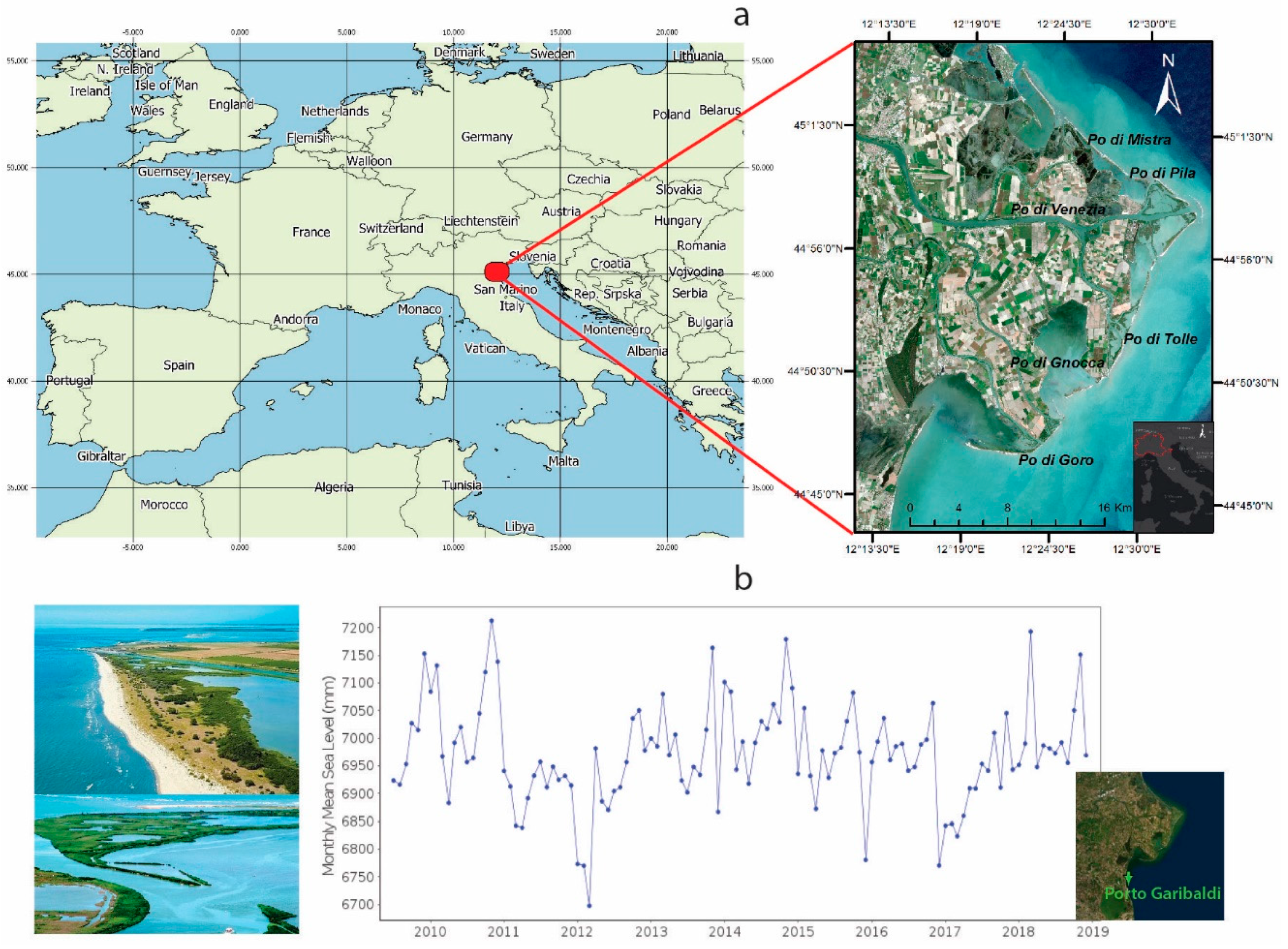
2.1. Study Area: Po Delta

The study focuses on the Po River Delta, the largest delta in Italy, which, like other major world deltas, is highly threatened by SLR [56,57,58,59] and natural subsidence (i.e., tectonic, sediment loading and sediment compaction) enhanced by anthropic activities (i.e., groundwater and methane extraction, drainage, and intensive farming practices) [60], making this coastal environment greatly vulnerable to inundation and erosion [61]. One of the main features of this area in terms of geomorphological, economic, and cultural value is that the Po Delta (Figure 1a) [62] underwent many changes of shape [63] and uses throughout history but still represents one of the most productive and biodiversity-rich areas. The system of the Po Delta is a relatively young (~4000–5000 years) alluvial fan that progrades from the Pianura Padana to the Adriatic Sea. The Po Delta covers an area of about 400 km² that extends seaward for about 25 km and is divided into five active branches. It is characterized by many dune systems and barrier islands that are sometimes connected to spits that delimiting lagoon areas along its coastline. Taking into account its natural variability and complexity, it is considered to be one of the most important European natural areas. Accordingly, it encompasses areas of great natural beauty and monuments of historical interest and was included on the UNESCO World Heritage list in 1995. The actual landform of the Po Delta is the result of river sedimentation processes but also of manmade actions that, over the centuries, have regulated the waters and reclaimed the land. It is an asymmetric delta dominated by shore-parallel, southward advection of finer-grained sediments. This asymmetric setting is also due to the loss of hydraulic efficiency of the northern fluvial branches in favor to the three southern branches. Until the middle of the 20th century, progradation of the delta was noticeable due to the abundant sediment supply [63]. Moreover, in the past few decades, the natural rates of subsidence (i.e., tectonic, sediment loading, compaction of Holocene sediments) estimated to be 2–4 mm/year were enhanced by human activities (i.e., groundwater and methane extraction, sediment supplies, drainage, and intensive farming practices) and experienced as much as 3 m of land subsidence from the 1930s to the 1970s [60]. Elevated subsidence rates, decreasing sediment supply due to dam and reservoir interception, and sediment mining in the lower river course caused major delta erosion after the 1950s. Indeed, over the last 50 years, coastal erosion affects both the emerged and the submerged (prodelta) systems [64], and a marked reduction of sediment supply led to a fast degradation and shoreline retreat [65] accelerated by human activity [42]. Most significant changes in terms of land use and land cover evolution is represented by a decrease in saltmarshes and a broadening of agricultural areas [66]. Additionally, over the last century, an artificial surface significantly spread out, and natural swamp and salt marsh areas decreased by 85% [66]. These and other interventions have deeply modified the physical and ecological characteristics of the Po Delta, determining a drastic change in existing ecosystems, together with a general decrease in the standards of environmental quality. Furthermore, the delta evidences multiple threats that will probably be exacerbated in the following decades by the effects of climate change (acting on wave dynamics and sea level rise), with potential environmental and socioeconomic impacts. Natural gas withdrawal led to high subsidence rates in the Po Delta [67], and large areas of the delta are now more than two meters below sea level, which is expected to have significant impacts related to increasingly SLR throughout the 21st century [13,33].

Observed SLR trends from tide gauge data between 2010 and 2019 also showed a general rise in the Adriatic Sea level, which ranges from 6.7 cm to 7.2 cm [68,69,70,71]. This situation is particularly alarming for the coastal restoration, mostly in the areas around the Po River Delta [9,33,66]. Indeed, the SLR [68,69] expected over the next 40–50 years will accentuate the transgressive phenomenon.

Together with the aforementioned aspects making this region particularly vulnerable to coastal erosion and flooding, anthropic pressures (e.g., tourism, industry, and fishery) and the effect of climate change (acting on wave dynamics and sea-level rise) are expected to affect the mobilization of sediments along the shoreline in the next few decades, with potential environmental and socioeconomic impacts [13]. At the delta-plain scale, many studies have already evaluated the potential impacts and vulnerability aspects, including the consideration of most relevant deltaic processes [19,72], among them natural and anthropogenic subsidence rates [33,60,66,73] and related relative sea level rise (RSLR) [33,59,73,74], changes in the land use [66], and coastal erosion processes [9,13]. Despite the fact that it has been demonstrated that the Po River has resumed delta progradation since 2010, this has occurred especially in its northern portion [65], highlighting the fact that the analysis of spatial and temporal vulnerability variations is required, since processes are spatially non-uniform.

2.2. Vulnerability Assessment

Coastal vulnerability assessment is a capable method for accounting for the interaction of the multiple environmental threats that determine a delta’s exposure [75,76]. BBN models have been chosen as a proper method for scenario simulations because they can assimilate different data distributions, including categorical, discrete, and continuous data.

Indeed, once BBN is trained, it is able to answer the following question: “What is the probability of target class (i.e., vulnerability), given the input distribution for the considered parameters under diverse sea level rise scenarios?” Once the probability that answers this question is calculated for every spatial units (cells) in the entire study area, a GIS-based probable vulnerability map is generated to produce belief maps based on the exploratory analysis of BBNs.

To characterize the vulnerability conditions of the study area by merging different kinds of variables from multiple data sources, a procedure made of several methodological phases has been developed (Figure 2). These phases include (1) data input, what includes definition, categorization, and homogenization of the variables; (2) BBN model design, which includes the organization of conditional probabilities between variables; and (3) vulnerability assessment, which includes the testing scenarios and the sensitive analysis.

First, all layers were clipped on the Po Delta study area, considering only natural and social subsystems, for removing data outside the purpose of the investigation (i.e., artificial surfaces and agricultural areas). The dimension of the spatial units were selected at the beginning of the assessment, based on the purpose of the analysis and on the spatial resolution of the available data. Our aim was to generate assessment units that will respond uniformly in terms of probable vulnerability and can be treated as single units for the purpose of adaptation or intervention planning in the future. We created a set of spatial coastal assessment units considering the radius of influence of coastal erosion (RICE area) as the landward limit [9,13,30]. According to the EUROSION definition, RICE is represented by a buffer of 500 m from the coastline extended to areas lying below −5 m [35,57], and it is considered as a proxy of the terrestrial areas, which may potentially be subject to coastal erosion or flooding in the coming period of 100 years. The threshold representing the RICE was set equal to 1 km inland on the Po Delta, as proposed in Gallina et al. [13] for the northern Adriatic area, covering a total delta surface of 64 km² and 62 km of the coastline. Likewise, the delta is split into three macro-sectors (Figure 3a) considering diverse coast orientation based on main wave climate [77] as the distribution of wave height, period, and direction averaged over a period of time (i.e., 2007–2017). Each macro-sector was divided into homogenous 500-m-long segments along the coastline (Figure 3b,c). Overall, there are 115 cells with an average length of 500 m and a width of 1 km, which have been overlaid with vulnerability assessment input data. To test the network, we explored several cases where we constrained the model with specific SLR scenarios, evaluating the probability of vulnerability, given a specified 100% probability that the rate of SLR refers exactly to each of the four diverse scenarios as described in Section 2.5 (Table 2).

2.3. Data Input

The identification of datasets counts on a broad availability of EO data processed by the authors and of already processed products from the European Copernicus Land Monitoring Service (CLMS) and the Copernicus Marine Environment Monitoring Service (CMEMS). This study takes into account other data sources including a variety of physical, ecological, and social variables to characterize the spatial pattern and the frequency distribution of the coastal vulnerability model.

Twelve variables are identified as relevant for simulating deltaic vulnerability scenarios, bearing in mind that delta systems are rapidly developing areas with changing landforms, sediment deposition rates, and vegetation cover. The physical, ecological, and social variables have been grouped in three broad classes representing the sources (driver factors–DFs), the pathway (land cover factors—LCFs), and the receptors (land use factors—LUFs) of the vulnerability [78,79] (respectively colored in red, green, and blue in

Table 1. List of input variables used in the Bayesian belief network (BBN) and description.

Variables (and Periods)	Description	Data Type	Processing Method and Data Source
Elevation (2007)	The elevation of the area is partially below mean sea level (msl) due to subsidence induced by hydraulic engineering works, extraction of gas-bearing water, and reduction of sediment supply and embanking.	EO-derived raster, continuous, terrestrial, 10-m-cell grid, digital elevation model (DEM).	DEM obtained from the achievement of the DIGITALIA project of Istituto Nazionale di Geofisica e Vulcanologia, INGV [89] Data source: http://www.pi.ingv.it/banche-dati/
Vertical velocity * (2003–2010)	The average vertical velocity represents a driver factor in terms of changes in rates of subsidence as well as it is a measure of the uncertainty in the erosion and flooding processes estimation.	EO-derived raster, continuous, terrestrial, 100-m-cell grid.	SBAS SARscape version 5.0.001 and ENVI version 5.0 (service pack 3). Data source: ESA Cat1 Envisat data access.
Waves (2007–2017)	Significant wave height and frequency are considered as proxy driver of coastal erosion summarizing the wave energy and wave impact. Three dominant wave directions were used considering the coastline shape and orientation of the study area: north (0–60°), center (60–120°) and south (120–180°).	Waves model derived points, discrete, aquatic, H0 = height, energy-based derived from significant wave height; and H0f = frequency, number of events related to the wave height.	Wave model transformed, with offshore wave rider buoy data (lat: 44.729168 lon: 12.833333), into nearshore equivalent significant wave height, direction and frequency. Data source: CMEMS.
Regime * (2010)	The regimes represent different levels of impact, depending on waves and coastal morphology, with thresholds indicating where processes and magnitudes of impacts change.	Calculated value using DEM and waves model derived points, discrete, terrestrial, topography transect based.	Runup parameterization Equation (1) applied to 115 topographic transects. Data source: elevation and waves.
Sea Level Rise (SLR) (2000–2100)	Future SLR scenarios, in this study, are classified as conservative, pessimistic and highly pessimistic scenario within 100 years.	Discrete, aquatic, added to the waves model derived points.	Added to height, energy-based derived from significant wave height of + 0.52 m and 0.74 m. Data source: [56].
Dune (2018)	Dunes and wetlands have a buffering capacity to reduce the adverse impacts of climate change in terms of natural barriers and responding capacity to SLR and erosion.	Vectorial polygons classified as dune and wetlands presence or absence, discrete, terrestrial.	Cover type classified as dune from regional Corine Land Cover (CLC) 2018 level 4 [30]. Data source: CLMS.
Coverage Factor * (2018)	The coverage factor stands for vegetation presence and abundance assuming that the susceptibility to erosion decrease with vegetation coverage due to higher wave energy dissipation.	Raster of the coastal buffer vegetation fractional abundance, continuous, terrestrial, 20-m-cell grid.	Sentinel 2 MSI satellite data processed with LSMA. Data source: https://scihub.copernicus.eu/
Protective Distance * (1991–2019)	The mean value of the maximum sediment spatial variations in the last 30 years is considered as the potential protective distance acting as a defense buffer against erosion processes. It is related to the dune presence and to the deltaic small-scale coastline changes.	Raster of the alongshore averaged values of the coastline sediment variation in the last 30 years, continuous, terrestrial, 30-m-cell grid.	Landsat (19912015) and Sentinel (2015–2019) satellite data processed with LSMA and EOF techniques. Data sources: https://earthexplorer.usgs.gov/; https://scihub.copernicus.eu/.
Geomorphology (1990–2005)	The geomorphology classifies the geomorphological and sedimentological elements of the shore in six major types: rocky, beaches, muddy, estuaries, harbors, and artificial coast.	Vectorial shore classified as geomorpho-sedimentological types, discrete, terrestrial-intertidal.	Based on the European coastline at scale 1:100,000 and CORINE Coastal Erosion version 1 updated after 1990. Data source: http://www.eurosion.org/database/geomorphology.html.
Global Surface Water Dynamic (GSVD) (1984–2015)	The GSVD represents where and when open water was present in 32 years. The transitions map represents the changes in water classes like no water, seasonal, permanent. The Occurrence Change map shows where surface water occurrence increased, decreased or remained constant.	Raster, continuous, aquatic, 30-m-cell grid divided in two 15-year time span.	The spatial and temporal variability of global surface water presence and its long-term changes (i.e., 32 years) calculated on 3 million Landsat images [90]. Data source: https://global-surface-water.appspot.com/.
Protected natural area (2010)	The network of core natural habitat types represents the natural capital of the area and corresponds to high exposure levels.	Vectorial polygons classified as protection designation, discrete, terrestrial.	It is the Natura 2000 network based on the Habitat and Birds Directives reporting and designation. Data source: CLMS.
Resilience Index (2017)	The resilience index is referred to the adaptive capacity of the Po Delta social subsystem and it involves socio-economic factors that affect community resilience at municipality scale.	Vectorial points at municipality scale, classified as degree of resilience, discrete, terrestrial.	Metrics obtained from stakeholders’ interviews, to score infrastructure and environment resilience’s subcomponents. Data source: [88].

* Processed by the authors.

).

It was assumed that the susceptibility to erosion decreases if the soil has high vegetative cover that contributes to higher wave energy dissipation. In response to rising sea levels and subsidence and diminishing fluvial sediment discharge [4], most deltas would naturally reduce their size under wave forces and migrate to shallow parts of the basin by switching or inundation. The deltaic fringe (i.e., subaerial and subaqueous parts of the deltaic coast interacting with and being modified by waves, tides, and currents) responds by barrier and dune buildup and sediment redistribution. Areas with less vegetation coverage were then assumed to be more susceptible (less resilient) to coastal erosion than wider vegetated areas [13].

In Table 1, the 12 variables are listed and described, highlighting data source types and formats, spatial resolutions, and temporal coverage. The use of multitemporal data acquired allowed for exploring diverse surface physical processes involved in the Po Delta dynamics. The use of an EO time series dataset from seven to 30-year timespans (Table 1) depends on the observed phenomena and on the objective of the data analysis. The case of vegetation and sediment dynamics led the use of a 30-year timespan for the analysis and classification of images considering the annual and seasonal change detection goal. Specifically, it allows us to identify land cover transitions and confirms the assumption of a high rate of changing conditions. All the continuous, raster variables are harmonized by a spatial resampling to obtain 100-m-cell grid resolutions and, in addition to the vector data, have been clipped on the reference study area buffer (RICE area).

Among the 12 variables, the vertical velocity was obtained using an EO radar dataset coming from the Envisat ASAR satellite sensor (2003–2010) with the small baseline subset (SBAS) technique and kriging interpolation. The variable is determined by the combination of ascending and descending line of sight (LOS) velocities. The vertical displacements velocity map is derived by interpolation (kriging) of points for a regular 100-m-cell grid.

The other large processing was the EO optical dataset based on Landsat and Sentinel 2 satellite datasets (1990–2019) with the linear spectral mixture analyses (LSMA) technique [80,81] (Tables S1 and S2). A 30-year stack of images derived from the two satellite sensors, geometrically and atmospherically corrected, was first masked to keep only the coastal land and the very shallow waters and discard sea and lagoon areas that surround the barrier islands. The LSMA processing to retrieve from the mixed reflectance signal of each pixel the fractional coverage abundance of sediments, vegetation, and water (dark) was based on a three multitemporal endmembers and fully constrained spectral mixture model on a regular 30-m-cell grid, as done in Filipponi et al. [81]. The derived variables called coverage factor and protective distance stand for the vegetation and sediment fractional abundance and are used as cover percentage maps to provide proxies for wave energy dissipation factor and coastal erosion protection [25]. In particular, the protective distance variable is obtained by calculating the empirical orthogonal function (EOF) of the 30-year layer stack, as done in Filipponi et al. [82], to obtain the temporal signal decomposition into dominant variability and to extract the most common variations sediment spatial patterns and temporal trends. The EOF technique was used to discriminate seasonal changes from the inter annuals and the alongshore averaged value of the maximum sediment variation in the last 30 years was considered as the potential protective distance acting as a defense buffer against erosion processes [83].

In order to have a complete source–pathway–receptor–consequence chain [54], the action of offshore waves were propagated down to each of the three coastal orientation and 115 cells (Figure 3c) to generate a point matrix with the frequency distribution of wave height, period, and direction averaged over the period of the analysis (2007–2017).

The waves were used in conjunction with the DEM to obtain the impact scale classification as in Sallenger et al. [14] to define four regimes representing different levels of impact and thresholds defining where processes and magnitudes of impacts change dramatically. The regime is calculated using the general expression Equation (1) for beach run up parameterization [15] applied to the 115 transects orthogonal to the shoreline spaced of 500 m, representing topographic variability along the coastline for each defined segment:

$${\mathrm{R}}^2=1.1\left(0.35{\mathrm{B}}_{\mathrm{f}}{\left({\mathrm{H}}_0{\mathrm{L}}_0\right)}^{1/2}+\frac{{\left[{\mathrm{H}}_0{\mathrm{L}}_0\left(0.563{\mathsf{\beta }}_{\mathrm{f}}^2+0.004\right)\right]}^{1/2}}{2}\right)$$

(1)

where H₀ = wave height; L₀ = deep-water wave length; β_f = beach steepness; and T_p = wave period calculated using the empirical formula Equation (2) [84,85,86]:

$${\mathrm{T}}_{\mathrm{p}}=1.32{\mathrm{H}}_{\mathrm{s}}+3.86$$

(2)

where H_s = significant wave height.

In accordance with Sallenget et al. [14], susceptibility to erosion (and consequently vulnerability) is higher for “inundation” regime where surge is sufficient to completely and continuously submerge the barrier islands. In the case of “overwash” regime, wave runup overtops the berm or, if present, the foredune ridge, and the associated net landward sand transport contributes to net migration of the barrier landward. Runup exceeds the threshold of the base of the foredune ridge in the “collision” regime, while in the “swash” regime runup is confined to the foreshore.

The adaptive capacity of the social systems depends on space and functioning organization, social and economic development, government and governance structure, and the presence of institutions that collect and store knowledge and experiences [87]. Here, adaptive capacity of the Po Delta social subsystem is posed by the resilience index [88], involving socio-economic factors that affect community resilience at the municipality scale, this being the primary administrative unit in case of emergencies and strategic in the urban planning activities. Specifically, it defines the metrics for community resilience drivers customized for the Po Delta from stakeholders’ interviews and states the variables able to measure social, economic, community capacity, infrastructure, and environment resilience subcomponents, proposing a list of factors indicated by the literature as appropriate for the resilience concept clustered into relevant dimensions.

2.4. BBN Model Design

BBN models based on probabilistic structure are best suited to perform scenario analysis such as quantitative vulnerability and risk analysis, error propagation, and decision making, while traditional deterministic modelling cannot provide the sophisticated spatial analytics required to model uncertainty within the natural environment. There are four main benefits to using BBNs compare to other methods. The ability to include uncertain or unavailable input variables coupled with expert knowledge makes BBNs a very powerful tool in decision support systems. Second, they describe relationships of causes and effects using a graphical framework (Phase 2) that provides for quantification of probabilities and clear communication of the results among scientists, managers, and the broader community, improving the integration of probabilistic modelling into adaptive management practices. Third, BNNs incorporate an explicit causal structure having more variables that interact directly and indirectly (Phases 3 and 4). Finally, BBNs perform computationally fast uncertainty assessments in complex systems and therefore are ideally suited for a spatial vulnerability trends distribution modelling, improving models’ predictive capability, where results are consistent if the aim is the definition of the maximum and minimum conditions of vulnerability (Phase 5).

It is important to be aware of the system complexity when building a Bayesian belief network (BBN); thus, constructing a model network first involves defining the purpose of the modelling and the variables that best describe the process to be studied in order to identify the relationship between the variables (which variables are impacted by which variables) and illustrating the relevance of some factors over others. The model network was designed with the 12 selected variables to address the most probable vulnerable areas following difference phases (Figure 2).

• Phase 1. The categorization phase involved an extensive literature review and expert consultations on the key variables and their relationships. The discretization was based on defining the number of intervals for each input variable by choosing thresholds computed using exploratory geo-statistics according to one of the three following criteria: (i) equidistant intervals, where each interval has the same width; (ii) quantiles or percentile, where each interval tends to have the same number of elements; and (iii) expertise or literature-review-based intervals, where the user defines the upper and lower limits of each interval. Accordingly, the states of a variable have been defined by translating parameter intervals in corresponding categorical (e.g., very low, low, moderate, high) or Boolean (i.e., yes/no) values (Figure 4). Based on the discrete quantities, a score from 1 to 4 contributing in increasing the final probable vulnerability has been assigned.

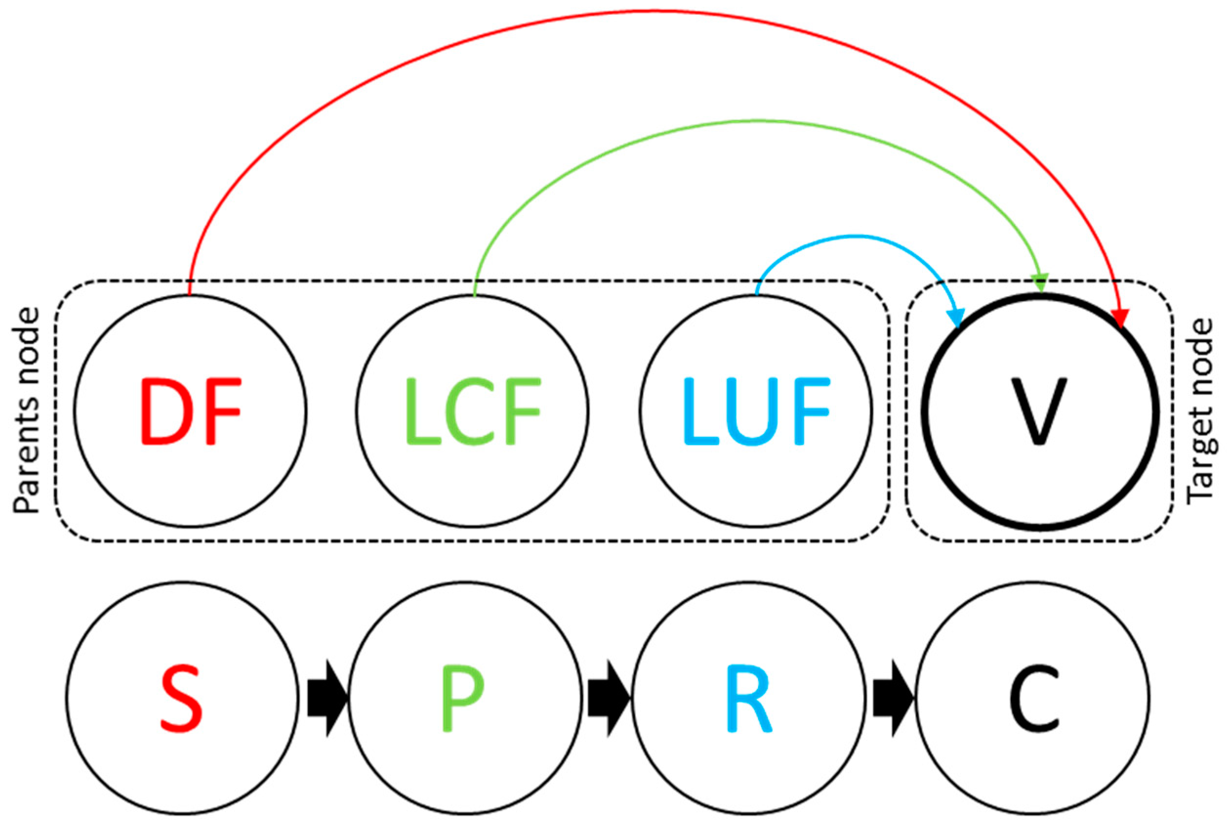
• Phase 2. A generic conceptual model (Figure 5) was used to develop an integrated network able to represent the relationships between input variables and the interconnection with source–pathway–receptor–consequence (SPRC) model applied to the vulnerability assessment. BBN is a directed acyclic graph (DAG) where the selected variables are represented by nodes and the arrows indicate the direct cause–effect relationships between the nodes [91] (Figure 5). The network is solved when nodes have been updated using Bayes’ Rule Equation (3):

  $$\mathrm{P}\left(\mathrm{A}|\mathrm{B}\right)=\mathrm{P}\left(\mathrm{B}|\mathrm{A}\right)\mathrm{P}\left(\mathrm{A}\right)/\mathrm{P}\left(\mathrm{B}\right)$$

  (3)

  where P(A) is the prior distribution of parameter A; P(A|B) is the posterior distribution, the probability of A given new data B; and P(B|A) the likelihood function, the probability of B given existing data A. Our hypothesis is that the functional relationship can be learned from available data set and cast in terms of a probabilistic estimate in the form Equation (4):

  $$\mathrm{P}(\mathrm{V}|\left\{\mathrm{DF},\mathrm{LCF},\mathrm{LUF}\right\}=\mathrm{f}\left[\mathrm{P}\left(\mathrm{DF},\mathrm{LCF},\mathrm{LUF}\right)\right]$$

  (4)

The conditional probability distribution of the Vulnerability (V), that is the “child node,” to a particular set of inputs variables can be obtained from the joint probability of driver factors (DFs), land cover factors (LCFs), and land use factors (LUFs) that are the “parents nodes”.

• Phase 3. To construct the BBN, the GeNie Academic Version 2.4 software package (BayesFusion, LCC, Pittsburgh, PA, US) was chosen. Classes corresponding to assigned score categories as described above resolve each parent or child node. The connection of each node in the BBN is determined by the conditional probability table (CPT) and probability table (PT), where the degree of belief (probability) that a variable will be in a particular state given the state of the parent variable [93] is defined.
• Phase 4. The entries in the CPTs and PTs can be discovered using a range and combination of methods, including directly observed data and probabilistic or empirical equations, results from model simulations and elicitation from expert knowledge. Some of the parameter learning functions are also based on expectation maximization (EM) algorithm (i.e., it requires only the model structure to be known beforehand and iteratively calculates maximum likelihood estimates for the parameters given the data and the model structure [38]) available in GeNie [94], implemented to provide prior probability for root nodes, while target node conditional probabilities is reported as a specific matrix representing the frequency of vulnerability scores associated with each input variables from one to four per cell. Vulnerability is selected as target node, the output variable that directly represents the phenomenon [92] (Figure 5). The prior probability is provided for regime, vertical velocity, dune, protective distance, coverage factor, global water surface dynamic, protected natural areas, and resilience index.
• Phase 5. Accordingly, the output of running the network contains the posterior probability distribution of the vulnerability node implementing extracted and reclassified values from resampling a GIS-based data set at 100 × 100 m resolution.

2.5. Vulnerability Assessment

The optimized model was used to predict vulnerability probability for the present SLR scenario and then for the three future SLR scenarios [56]. Once parameters have been learnt, a prediction can be made by updating the BBN with “evidence,” whereby the states of SLR node in the systems assume certain probabilities and the resultant conditional probabilities of the target variable are estimated. Vulnerability worst-case projection of global mean SLR to 100 years [56] (the highly pessimistic) has been considered (i.e., the more precautionary conditions). Three SLR future scenarios have been finally implemented in the BBN as evidence (

Table 2. Mean values of the Intergovernmental Panel on Climate Change (IPCC) SLR prospected for the next 100 years to best- and worst-case conditions.

Scenarios	Sea Level Rise (IPCC, 2014)
Present	0.00 m
Conservative	0.52 m
Pessimistic	0.74 m
Highly Pessimistic	0.98 m

): conservative scenario, pessimistic scenario, and highly pessimistic scenario. In the testing phase, many factors such as changes in wave height are characterized by high uncertainty in the northern Adriatic [57,58]. Except for the value of SLR, the values of all the other variables are assumed to be unchanged in hundred years, even average vertical velocity and surface water dynamics are considered in accordance with the present trends.

Starting from posterior vulnerability probability obtained from BBNs models testing scenarios, the hotspot areas of the study coast are identified.

2.6. Sensitive Analysis

Broadly, in a Bayesian network, the sensitivity analysis refers to the analysis of the influence and influence degrees of multiple causes (node states) on the result (target node) [38,95]. The sensitivity analysis function of GeNie 2.4 can be used to identify which variables in the system have the highest influence on the outcome of the model. This is done by investigating the effect of small changes in numerical parameters (i.e., probabilities) on the output parameters (e.g., posterior probabilities). Highly sensitive parameters affect the reasoning results more significantly having the highest influence on the delta vulnerability target node. GeNIe implements an algorithm proposed by Gaag et al. [96] that performs simple sensitivity analysis in Bayesian networks. The algorithm efficiently calculates a complete set of derivatives (i.e., the value of the first derivative of the posterior probability of the selected state of the target node at its current value over the considered parameter) of the posterior probability distributions over the target node over each of the numerical parameters of the Bayesian network. These derivatives give an indication of importance of precision of network numerical parameters for calculating the posterior probabilities of the target. If the derivative is large for a parameter, then a small change in that parameter may lead to a large change in the posteriors of the target variable. If the derivative is small, then even large changes in the parameter make little difference in the posteriors. The tornado plot of the sensitivity test shows the most sensitive parameters for a selected state of the target node sorted from the most to least sensitive.

Strength of influence is calculated from the CPT of the child node and essentially expresses some form of distance between the various conditional probability distributions over the child node conditional on the states of the parent node taking the plain average over distances in the normalized mode.

3. Results

3.1. Data Input Discretization

Input variables have been transformed in categorical scales, and a score, ranging from 1 (low vulnerability) to 4 (high vulnerability), was assigned to each variables’ category (

Table 3. Summary of variables included in the BBN, discretization methods applied and distribution classes, intervals, scores and states associated with the input variables identified in the vulnerability matrix for BBN model in the Po Delta area colored based on the types of variables representing the sources, driver factor (red), the pathway, land cover factor (green), the receptors, land use factor (blue). A score of 1 means a very low contribution to vulnerability, and a value of 4 means a high contribution to vulnerability.

Input Variables		Discretization Method and Main Distribution Results	Interval	Score	State
Elevation		Expert decision/literature review   Elevation above sea level represent the 38% of emerged areas, mostly concentrated in the northern macro-sector. The central and southern macro-sectors emerged areas are mostly below sea level reaching elevation values of −3 m above sea level in some specific sectors.	>1 m	1	Very Low
			0 m–−1 m	2	Low
			−1 m–0 m	3	Moderate
			−3 mm/year–−1 m	4	High
Vertical velocity		Expert decision/literature review   Vertical velocity reaches the maximum value values in the area of Porto Tolle, Po di Goro (average rates of ~9–10 mm/year), despite the null values observed in the inland area	>−1 mm/year	1	Very Low
			−2.5 mm/year–−1 mm/year	2	Low
			−4.1 mm/year–−2.5 mm/year	3	Moderate
			<−4.1 mm/year	4	High
Waves	H0 Height	Expert decision   H0 raging between 0.2 and 1 m represents the 87% of the occurred events, while the 12% of the events was classified between 1–2 m and the 1% as greater than 2 m.	0.2 m–1 m	2	Low
			1 m–2 m	3	Moderate
			>2 m	4	High
	H0 Frequency	Percentile   The 53% and 15% of the events occurred in the central and southern macro-sectors respectively, while 2017 the 32% of the events occurred in the northern macro-sector.	571 events–6771 events	1	Low
			6771 events–12,970 events	2	Moderate
			>12,970 events	3	High
Regime		Equal intervals/literature review   In the northern macro-sector 9.7 km2 could be characterized by the “collision” regime, whilst 6.4 km2 could be characterized by the “overwash” regime. In the central part of the delta “collision” regime is more probable north of Po di Pila mouth, while the “overwash” regime is expected in the sector adjacent and south of Po di Pila mouth. In the southern part of the study area ‘collision’ regime is more probable, while along the coastline located close to Po di Tolle mouth, the occurrence of the “overwash” regime is expected.	−1–−0.5	1	Very
			−0.5–0	2	Low
			0–0.5	3	Moderate
			0.5–1	4	High
Sea Level Rise		Expert decision/literature review   Three SLR future scenarios have been classified in: present scenario, conservative scenario, pessimistic scenario and highly pessimistic scenario.	0.13 m	1	Present
			0.52 m	2	Conservative
			0.74 m	3	Pessimistic
			0.98 m	4	Highly Pessimistic
Dune		Expert decision   Dune coverage an area of 5.2 km2 of which 2.3 km2 in the northern macro-sector, 0.7 km2 in the central macro-sector and the other 2.2 km2 in the southern macro-sector.	Presence	1	Yes
			Absence	4	No
Coverage Factor		Percentile   The cover map based on the per-pixel vegetation abundance obtained with the LSMA, the average value of the vegetation abundance (AVA) in % of the pixels that each polygon contains has been calculated, obtaining 45% as the maximum AVA. The final cover map differs between vegetated and non-vegetated emerged areas, depending on the AVA being higher or lower than the 50th percentile. Mapped vegetated areas are mostly distributed close to Po di Mistra, Po di Pila, and Po di Tolle and south of Po di Goro.	>16.65%	1	Yes
			≤16.65%	4	No
Protective Distance		Equal intervals   The potential protective distance acting as a defense buffer against erosion processes obtained using the EOF approach, divided in four classes, from less than 40 m up to 1500 m. The highest values are found along the coastline, between Po di Mistra and Po di Pila mouths, and in the southern part, close to Lido di Volano.	>1500 m	1	Very Low
			1500 m–230 m	2	Low
			230 m–40 m	3	Moderate
			<40 m	4	High
Geomorphology		Expert Decision   21.8 km of the coastline were classified as developed beaches of which 4.6 km located in the northern macro-sector, whilst 38.4 km are classified as non-cohesive sediments of which 13.6 km located in the northern, 18.2 km located in the southern. The central macro-sector is completely characterized by non-cohesive sediments.	Soft non-cohesive sediments	2	Low
			Developed beaches (<1 km long)	4	High
Global Surface Water Dynamic	Water Transition	Expert Decision   In the central macro-sector in correspondence of Po di Pila mouth, a loss of permanent water is observed as a consequence of conversion of permanent water into land. Rather, in the southern macro-sector close to the Po di Gnocca mouth land converted into seasonal water, while in correspondence of the sandy spit (the Scanno in Sacca di Goro) located south of Po di Goro mouth a loss of permanent water occurred.	0–110%	1	Very Low
			111–142%	2	Low
			143–177%	3	Moderate
			178–200%	4	High
	Surface Water Occurrence Change Intensity	Expert Decision   Surface water occurrence changes are mainly distributed along the coastline higher intensity of surface water occurrence change, where the surface water occurrence decreased across the 32 years period, located in the central macro-sector in correspondence of Po di Pila mouth. In the southern macro-sector, water occurrence increased more intensely close to the Po di Gnocca mouth and decrease in correspondence of the sandy spit (The Scanno in Sacca di Goro) located south of Po di Goro mouth.	-Permanent water surfaces, no change   -Conversion of permanent water into land   -Conversion of a seasonal water into land	1	Very Low
			-Seasonal water surfaces, no change   -Land replaced by permanent or seasonal water that subsequently disappears	2	Low
			-Conversion of land or permanent water into seasonal water	3	Moderate
			-Conversion of land or seasonal water into permanent water	4	High
Protected natural area		Expert decision   The 57% of the study area is classified as “protected” according to Natura2000. In the northern macro-sector, 8.2 km2 of a total 19.1 km2 are classified as protected areas. In the central macro-sector 4.3 km2 are protected areas on 8.1 km2. In the southern macro-sector, protected areas cover 24.6 km2 of a total of 37 km2.	Absence	1	No
			Presence	4	Yes
Resilience Index		Percentile   The average, maximum and minimum values obtained are 4.2, 5.1 recorded in Rosolina, and 3.2 recorded in Goro, respectively. Higher values mean greater resilience resulting in lower vulnerability. In the Rosolina municipality, higher values of infrastructure and social resilience subcomponents (equal to 1) led to a higher index value.	>4.3	1	Very Low
			3.5–4.3	2	Low
			3.2–3.5	3	Moderate
			<3–2	4	High

).

3.2. BBN Model

To address the question of how vulnerable the Po Delta sub-systems are, we provided a probabilistic prediction giving the (in) dependence relationships among the variables and between variables and the target node, designing a BBN graphical model using a DAG.

The resulting graphical network (Figure 6), derived from the hypothesis that the vulnerability is a function of 12 input variables having 1537 possible combinations of input variable states. The target node conditional probabilities matrix represents the frequency of vulnerability scores associated with each input variables with values from one to four per cell.

3.3. Testing Scenarios

Figure S1 reports two of the four testing scenarios applied to the whole delta for present and highly pessimistic scenarios.

Focusing on reference present scenario at macro-sector scale (Figure 7), probability of “high” vulnerability accounts for the 7%, 22%, and over the 7% for the northern, central and southern macro-sectors, respectively. The probability of “moderate” vulnerability constitutes the 22% of both central and southern macro-sectors, and the 36% of the northern. Looking at “low” vulnerability, the variability of probability among macro-sectors is smaller, being 24%, 22%, and 22% for the northern, central, and southern areas, respectively. “Very low” vulnerability shows probability values equal to 33% for all the macro-sectors. Focusing on the highly pessimistic scenario at macro-sector scale a growing probability of “high” vulnerability is evident, increasing at 24%, 38%, and 24% for the northern, central, and southern macro-sectors, respectively, to the detriment of the “moderate” vulnerability probability category.

The probability of “moderate” vulnerability noticeably increased in the pessimistic scenario resulting in 52%, 40%, and 54% for the northern, central, and southern macro-sectors, respectively, to the detriment of the “low” vulnerability probability category.

The characteristic behaviors of the vulnerabilities for each SLR scenario along each of the 115 cells divided in three macro-sectors is represented in Figure 8. As expected, the results show mostly a constant increase of 16–17% of probability of “high” vulnerability comparing the present and highly pessimistic scenarios. Taking as a reference the present scenario and looking at a conservative scenario projected SLR of 0.52 m, it appears that the overall vulnerability of the delta will not change considerably within 100 years, and “low” vulnerability probability increases at the expenses of “very low” vulnerability probability across all the three macro-sectors. Looking at a pessimistic scenario projected SLR of 0.74 m, the “moderate” probability of vulnerability rises almost 17 percentage points compared to reference scenario reaching 54% in the southern sectors and to almost 16% in the other sectors.

Vulnerability probability maps have been created by transferring the probabilistic results of vulnerability for each SLR scenario into the GIS environment (Figure 9) and by defining the level of probability in each cell identified in the Po Delta.

3.4. Identification of Hotspot Areas

The calculated vulnerability probability has allowed us to identify the hotspot areas.

The very low probability accounts for the northern sector and, as expected, the increasing SLR would reduce the low probability of vulnerability and even maintaining the spatial pattern due to the different exposure of the systems to the waves intensity and frequency.

It is of interest that the social resilience in the northern macro-sector is higher, and this is an influencing factor on the lower exposure of receptors (Figure 9a,e,i,m).

The low vulnerability probability has a heterogeneous pattern moving along the cells and, unless the central delta, the values never reach very high probability (>75%) (Figure 9b,f,j,n).

Moderate vulnerability probability highlights, as hot spots the southern Po Delta, where the sandy spits and barrier are the dominant typology of the coast, as with very relevant dune and wetlands habitat, determining higher receptors exposure due to the natural capital. The dunes and the saltmarshes do not reach elevations enabling a barrier role to the increasing SLR (Figure 9c,g,k,o).

High vulnerability probability is recurrent in the central delta that is the ebb area with a higher rate of changing conditions due the interaction between sediments and seawaters. Here, even the exposure is lower in respect to the northern and southern macro sectors, the elevation is the lower, the overwash regime dominates, and no adaptive factors are able to reduce the probability of vulnerability (Figure 9d,h,l,p).

3.5. Sensitivity Analysis

The results of sensitivity tests and the strength of influence for a “high” vulnerability state show that the elevation and the water occurrence dynamic affect the uncertainty of vulnerability the most (Figure 10). We found that, among variable waves, H₀ has the highest impacts on vulnerability. The other parameters seem to have the same degree of influence on the target variable, with lower values for protective distance variable. To analyze the sensitivity under the highly pessimistic SLR scenario, we used a tornado diagram to investigate the impacts on the “high” vulnerability state (vulnerability = high). The analysis provides the range (10% of its current value up and 10% down) and the direction (negative or positive) of changes in the target state. The most sensitive combination of the variables is regime = low; protective distance = low; protected areas = no; resilience = moderate; SLR = highly pessimistic; H₀ frequency = moderate (Figure S2).

4. Discussion

In light of increasing anthropogenic and climatic pressures and the uncertain future that climate change poses, especially related to SLR, there is an unmet need for information solutions and theories that can enable the effective implementation of risk mitigation measures in low-lying coastal areas [5]. The main objective of the analysis was to assess and map vulnerability with target classes (i.e., very low, low, moderate, or high vulnerability) to help decision makers in future planning and management actions, implementing coastal regulations, and recognizing high-priority intervention hot spots in natural and social subsystems. The peculiarity of the integrated approach described here lies in the extraction of vulnerability values using EO data directly implemented in a BBN model, with the key advantage of generating conditional probabilities on the past and present data and exploring several future SLR scenarios.

4.1. Data Input Relevance

With the aim to overcome previous model-driven tools’ weaknesses related to the capability of representing vulnerability on a spatial basis and variables mutual interactions, EO-based methods are suitable to include the complex physical and ecological variability of the Po Deltas’ patterns and processes [59,60,65,66,67]. The use of EO from satellites and Copernicus information along with modeling plays a key role in the provision of spatial products representing land surface attributes in a continuous way determining an advantage for a valuable data-driven approach and in coastal processes understanding. First, the combination of satellite data coupled with spatially referenced ancillary measures, including vegetation, topography and bathymetries, climate, and geology, [4,23,24,40,53,54,81,82,95], has proved to be a cost-effective approach to classify and quantify coastal parameters [23,53,54,82,83] influencing the delta’s vulnerability (Table 1 and Table 3). Second, the use of EO data contributes to a better understanding and regular monitoring of landforms and coastal dynamics. Specifically, the use of SAR-based interferometry for the monitoring of land subsidence reveals the heterogeneity of the subsidence rates along the coastal system, and the spatial pattern of this variable can be used as a source of vulnerability as well as a determinant of uncertainties in the interpretation of the relative sea level rise scenarios effects [33,59]. The use of an EO optical dataset based on Landsat and Sentinel 2 satellite 30-year data time series (Tables S1 and S2) definitely supports expert knowledge to deeply understand surface physical processes related to vegetation and sediments dynamics that highly influence the susceptibility to erosion processes across scales.

4.2. BBN Model Development

The use of BBNs allows the possibility to integrate variables acquired from different sources. Phase 1 of the model design accommodates the limited ability of BBNs to deal with continuous parameters derived from EO data input [38,39] and for running the model over the discrete sectors and subsectors, discretized values (i.e., from 2 to 4 intervals) treated as categorical (Figure 4) (Table 3). This allowed us to build a meaningful BBN and to capture complex empirical distributions and non-linear relationships among the variables. The BBN-developed model (Figure 5) is applied using current conditions, which define the baseline, using future SLR scenarios taking in consideration the Intergovernmental Panel on Climate Change SLR projections [56] to define a plausible future vulnerability probability occurrence. For each identified sector in the three macro-sectors, the values in the input data are used as evidence in the network, and inference is performed to obtain the posterior probability distribution of the target nodes (Figure 7 and Figure 8). Then, the posterior distributions of the target nodes are written into a spatial file making the results a combination of each cell (Figure 9). The simplicity of the links between variables in a BBN means that it is possible to model very complex systems and also to model these kinds of data with a different number of state variables [39]. Generally, in the BBN results, weaknesses emerge in the case of the arbitrary definition of conditional probabilities when expert knowledge is not available or there is a lack of “evidence” in terms of information on the intensity and extent of the past hazardous events and on the consequent damage impacts [63,65].

4.3. Vulnerability Assessment and Key Findings

The aim of mapping coastal vulnerability required running the BBN in a spatially explicit way able to include the spatial variability of the main coastal features, and the knowledge on the delta system allowed developing a segmentation of the coastal delta adopting as reference spatial boundary for vulnerability assessment [13,30,31,35,57,58] (Figure 3b,c) the landward limit of the radius of influence of coastal erosion (RICE) area.

The ongoing climatic changes will further intensify the present intensive erosive phenomena related to the reduction of fluvial discharges and subsidence [62,63]. Here, the results confirmed the outcome provided by Tosi et al. [59] using a multi-band SAR methodology integrating COSMO-SkyMed and ALOS-PALSAR images, since the subsidence rates increase eastward toward the central tip of the delta, mainly composed by unconsolidated, highly compressible thick prodelta mud. Consequently, there is a greater probability of high vulnerability hot spots in the central delta (Figure 9d), increasing in view of the highly pessimistic SLR scenario (Figure 9p). Human activities (i.e., drainage and intensive farming practices in the upstream portion of the delta [66], methane groundwater extractions, sediment supplies) have caused a worsening of the situation increasing subsidence rates related to natural consolidation of recent compressible low-permeable deposits [60,63,66] that, in view of the expected SLR, will continue to occur for decades in the portions of the Po Delta formed over the last two to three centuries [60]. Moreover, subsidence in concomitance with the heavy reduction of the sediment load of the Po and enhanced erosive phenomena [60,63], as observable in the reduced protective distance of southern sector, result in the greater percentage of moderate vulnerability probability hot spots in the current scenario (Figure 9) (Table 3). Here, the greater probability of moderate vulnerability is rather influenced by LUFs, and the low social resilience is particularly affected by low social and institutional resilience [88] and the extensive presence of protected natural areas.

Therefore, observing hot spots vulnerability variation in the whole delta, non-climatic environmental and human-induced (i.e., coverage factor, protective distance and subsidence) and socio-economic (i.e., resilience) variables turned out to be relevant in determining expected higher vulnerability (Figure 10) as for hot spots located in the central ebb area (Figure 7, Figure 8 and Figure 9). Indeed, hot spots placed in the central macro sector show higher rate of changing conditions due the interaction between sediments and seawaters [4,65]. Considering that the exposure is lower in respect to the northern and southern macro sectors, the elevation is the lower and no adaptive factors (i.e., here lower economic and institutional resilience components diminish the adaptive capacity) are able to reduce the probability of vulnerability (likewise confirmed by the sensitivity analysis shown in Figure S2), the use of the heterogeneity of the subsidence rates in the BBN analysis has been relevant.

Furthermore, the inclusion of the LCFs (i.e., coverage factor, dunes presence and geomorphology) (Table 1) contributes to explain the lower probability of high vulnerability for the majority of northern hot spots, with some exceptions for the northward hot spots (Figure 8 and Figure 9), where despite higher adaptive capacity and lower subsidence rates, exposure is significantly higher (i.e., the absence of dunes and sub-merged vegetation acting as proxy for wave energy dissipation, prevalence of overwash regime, lower protective distance and developed beaches < of 1 km) (Figure 4) (Table 3). Highly heterogeneity of vulnerability to SLR, resulting in significantly different probability values of contiguous cells, particularly visible in both “moderate” and “high” vulnerability maps (Figure 9), reflects the combined result of the spatialized variables derived from EO data. Although the sensitivity analysis (Figure S2) shows that vulnerability is more influenced by low energetic but more frequent events (Table 3), the frequency of storm-related erosive marine processes in the last decade has remained substantially constant, showing only limited deviation within the normal climate variability especially in the northern portion [65] and highlighting the importance to include the interaction between waves and coastal morphology to define potential impacts (i.e., regime). The results could be enriched by integrating the model flow with real cases (i.e., introducing “evidence”) and adding significant additional factors and their combined effects that are important on local scales (e.g., coastal structures, river discharge, total suspend matter, wetlands typology distribution, longshore transport, sediment budgets, hydrological modification and deforestation, changes in coastline, and coastal erosion) may significantly improve predictions of sites experiencing coastal vulnerability. In this view, introducing evidences and limitations by informing the CPTs with evidentiary data and outcome states could lead to an improvement of the effective variance reduction that mainly depends on the influence of each input variables to the network.

The 12 variables frequency distribution used to generate categories all across the stretch makes the cells only comparable to each other, for the results of the Po Delta study, and they are not comparable with other deltas of the world because the frequency distribution of values of other areas, even considering the same set of variables, would be significantly different.

4.4. Management Implications

We build on the current state of knowledge with an approach capable to support short to medium-term coastal management decisions in identifying key variables and their interactions [40], prioritizing areas that are vulnerable, and determining planning interventions considering natural and social subsystems, thus improving deterministic models, which remain arguable when applied to real cases [38,39]. The consideration of EO time series dataset and the involvement of relevant stakeholders address the re-thinking of existing policy and planning constraints and adaptation strategies. In interpreting model outcomes, BBN results confirm that this is a valuable tool for vulnerability assessment, since it can incorporate different typology of data—both quantitative (e.g., obtained from existing models, monitoring and from site-specific measurements) and qualitative—obtained mostly from expert stakeholder knowledge, providing a probability-based approach. In addition, the probabilistic and analytical structure of the variables network takes into account uncertainties, which are often high in vulnerability scenarios. The graphic representation (Figure 6 and Figure S1) enables a simplified communication for stakeholders and decision makers about the interaction among variables to the probability of vulnerability because (i) it makes easy deducing the probabilities of different causes given the consequences (Figure 10) and (ii) it provides fast responses to queries to decision makers, in contrast to simulation-based models that requires time and computational power [38]. Findings of the study put in evidence that the synergistic effects of various pressures, particularly human-induced processes, appear to exacerbate the increasing of high vulnerability in the perspective of a highly pessimistic SLR scenario, at least at the local scale. Consequently, the identification of hotspot areas and the preparation of a correct coastal vulnerability assessment to SLR need to take into consideration also non-climate drivers, in the perspective of a local-level model downscaling. The study also highlights the greatest strength in the use of the social-ecological components to address the natural and human capital exposed to future SLR. The resilience index in particular provided the stakeholders knowledge integration that is considered one of the most relevant inputs when building the BBN. The protected natural areas along with the coverage factor provided the inclusion of ecosystem services components as the variables that account for the naturalistic role of the delta and protection from erosion. Considering the CF as a key indicator, we can state that the socio-ecological resistance and resilience evaluation could be based on the interaction of the physical, biological, and social components.

5. Conclusions

From the obtained outcomes, we are able to draw the following main conclusions:

• EO satellite data keeps proving its high potential for monitoring the Earth, easing spatial and temporal analysis in very complex and dynamic areas.
• The implementation of EO data into the BBN model provides a statistical framework performing inference on a very large amount of different data that describes what is known about the physical, ecological, and social parameters of the system and, perhaps more importantly, what is known about the causal relationships between them.
• The BBN approach, based on the definition of conditional probabilities, associated to the use of a GIS tool, provided the trend of distributions of vulnerability along the shore, which is especially useful for management and planning purposes.
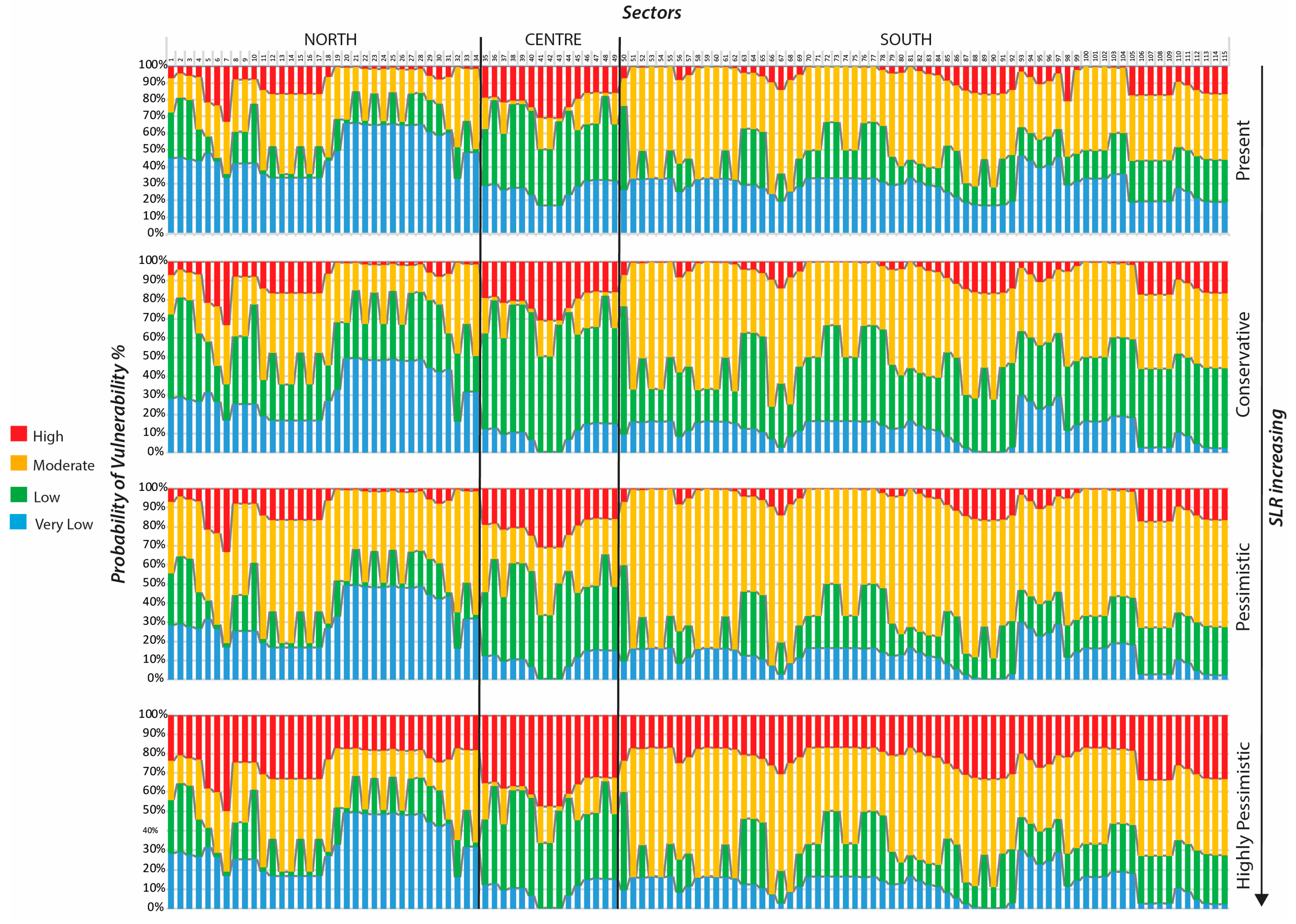
• The overall assessment reveals that almost the 35% of the Po Delta is highly vulnerable to the highly pessimistic SLR scenario. The high heterogeneity of vulnerability to SLR reflects the combined results of the selected variables: 29% of the northern cells, 100% of the central cells, and 23% of the southern cells fall into vulnerability target classes that range from 0.34% to >72% of probability to being highly vulnerable. Our findings highlight potential changes in the sediment budget considering the major vulnerability of the central ebb that is the gate between the river sediment supply and the costal sediment transport.
• The outcomes highlight the strength of influence of each variable on the target and their evident dependence and interconnection. Wave climate mostly depending on events frequency, land subsidence, and changes in land cover, which are the more sensitive variables playing a key role in vulnerability to SLR.
• The study mainly highlights the need (i) to update and expand coastal data sets, specifically concerning local scale environmental and human-induced processes, and (ii) to include both bio-geophysical and socio-economic aspects within delta analysis of the distribution and change in risk components, identifying vulnerable areas and communities, and where changes in hot spots may occur in the future. This can inform other analyses, such as the design of surveys and data collection, as well as identify policy needs and indicate where adaptation actions are likely to be required.
• The findings of this study are also valuable for the further performance of a gap analysis between the available tools and operational user needs. Emerged results provide a contribution in term of completeness of the information for a clearer overview of the expected vulnerability pattern and key variables. These insights could be useful to assess and verify the compliance and the capability of existing products to the user and stakeholder needs and to define a suitable strategy that could fulfil those needs.

The authors consider the study a definition of a spatially explicit tool for vulnerability assessment in deltaic systems and a contribution in terms of knowledge to the local management and planning component. This approach is a starting point for researchers and institutions to develop new down streaming services and evolve more detailed and scalable models to policies, with the aim of enhancing Earth monitoring and the detection of changes in coastal areas.

References

1. Ericson, J.P.; Vorosmarty, C.; Dingman, S.L.; Ward, L.G.; Meybeck, M. Effective sea-level rise and deltas: Causes of change and human dimension implications. Glob. Planet. Chang. 2006, 50, 63–82. [Google Scholar] [CrossRef]
2. Field, C.B.; Barros, V.R.; Dokken, D.J.; Mach, K.J.; Mastrandrea, M.D. Climate change 2014-impacts, adaptation and vulnerability: Part A: Global and sectoral aspects by intergovernmental panel on climate change. Impacts Adapt. Vulnerability 2014, 315–356. [Google Scholar] [CrossRef] [Green Version]
3. Ricaurte, L.F.; Olaya-Rodríguez, M.H.; Cepeda-Valencia, J.; Lara, D.; Arroyave-Suárez, J.; Finlayson, C.M.; Palomo, I. Future impacts of drivers of change on wetland ecosystem services in Colombia. Glob. Environ. Chang. 2017, 44, 158–169. [Google Scholar] [CrossRef]
4. Besset, M.; Anthony, E.J.; Sabatier, F. River delta shoreline reworking and erosion in the Mediterranean and Black Seas: The potential roles of fluvial sediment starvation and other factors. Elem. Sci. Anth. 2017, 5, 54. [Google Scholar] [CrossRef] [Green Version]
5. Wong, P.P.; Losada, I.J.; Gattuso, J.-P.; Hinkel, J.; Khattabi, A.; McInnes, K.L.; Saito, Y.; Sallenger, A. Coastal systems and low-lying areas. In Climate Change 2014: Impacts, Adaptation, and Vulnerability. Proceedings of the Part A: Global and Sectoral Aspects, Contribution of Working Group II to the Fifth Assessment Report of the Intergovernmental Panel on Climate Change; Cambridge University Press: Cambridge, UK; New York, NY, USA, 2014; pp. 361–409. [Google Scholar]
6. Szabo, S.; Brondizio, E.; Renaud, F.G.; Hetrick, S.; Nicholls, R.J.; Matthews, Z.; Tessler, Z.; Tejedor, A.; Sebesvari, Z.; Foufoula-Georgiou, E.; et al. Population dynamics, delta vulnerability and environmental change: Comparison of the Mekong, Ganges–Brahmaputra and Amazon delta regions. Sustain. Sci. 2016, 11, 539–554. [Google Scholar] [CrossRef] [PubMed] [Green Version]
7. Coleman, J.M.; Huh, O.K.; Braud Jr, D.H.; Roberts, H.H. Gulf. Coast. Assoc. Geol. Soc. 2006, 55, 102–131. [Google Scholar]
8. Coleman, J.M.; Huh, O.K.; Braud, D. Wetland loss in world deltas. J. Coast. Res. 2008, 1, 1–14. [Google Scholar] [CrossRef]
9. Torresan, S.; Gallina, V.; Gualdi, S.; Bellafiore, D.; Umgiesser, G.; Carniel, S.; Sclavo, M.; Benetazzo, A.; Giubilato, E.; Critto, A. Assessment of climate change impacts in the north Adriatic coastal area. Part I: A multi-model chain for the definition of climate change hazard scenarios. Water 2019, 11, 1157. [Google Scholar] [CrossRef] [Green Version]
10. Overeem, I.; Syvitski, J.P.M. Dynamics and vulnerability of delta systems. In LOICZ Reports Studies; GKSS Res. Center: Geesthacht, Germany, 2009; p. 54. [Google Scholar]
11. Woodroffe, C.D.; Nicholls, R.J.; Saito, Y.; Chen, Z.; Goodbred, S.L. Landscape Variability and the Response of Asian Megadeltas to Environmental Change BT-Global Change and Integrated Coastal Management: The Asia-Pacific Region; Harvey, N., Ed.; Springer: Dordrecht, The Netherland, 2006; pp. 277–314. ISBN 978-1-4020-3628-6. [Google Scholar]
12. Plant, N.; Thieler, E.R.; Passeri, D.L. Coupling centennial-scale shoreline change to sea-level rise and coastal morphology in the Gulf of Mexico using a Bayesian network. Earth’s Futur. 2016, 4, 143–158. [Google Scholar] [CrossRef] [Green Version]
13. Gallina, V.; Torresan, S.; Zabeo, A.; Rizzi, J.; Carniel, S.; Sclavo, M.; Pizzol, L.; Marcomini, A.; Critto, A. Assessment of climate change impacts in the north Adriatic coastal area. Part II: Consequences for coastal erosion impacts at the regional scale. Water 2019, 11, 1300. [Google Scholar] [CrossRef] [Green Version]
14. Sallenger, A.H. Storm impact scale for barrier islands. J. Coast. Res. 2000, 16, 890–895. [Google Scholar]
15. Stockdon, H.F.; Holman, R.A.; Howd, P.A.; Sallenger, A.H. Empirical parameterization of setup, swash, and runup. Coast. Eng. 2006, 53, 573–588. [Google Scholar] [CrossRef]
16. Sanuy, M.; Jiménez, J.; Plant, N. A Bayesian Network methodology for coastal hazard assessments on a regional scale: The BN-CRAF. Coast. Eng. 2020, 157, 103627. [Google Scholar] [CrossRef]
17. Taramelli, A.; Manzo, C.; Valentini, E.; Cornacchia, L. Coastal subsidence: Causes, mapping, and monitoring. In Natural Hazards: Earthquakes, Volcanoes, and Landslides; Ramesh Singh, D.B., Ed.; CRC Press: Boca Raton, FL, USA, 2018; pp. 253–290. ISBN 9781138054431. [Google Scholar]
18. Martinez, M.L.; Taramelli, A.; Silva, R. Resistance and resilience: Facing the multidimensional challenges in coastal areas. J. Coast. Res. 2017, 77, 1–6. [Google Scholar] [CrossRef]
19. Wolff, C.; Vafeidis, A.T.; Muis, S.; Lincke, D.; Satta, A.; Lionello, P.; Jiménez, J.; Conte, D.; Hinkel, J. A Mediterranean coastal database for assessing the impacts of sea-level rise and associated hazards. Sci. Data 2018, 5, 180044. [Google Scholar] [CrossRef] [Green Version]
20. Dadson, S.; Ashpole, I.; Harris, P.P.; Davies, H.N.; Clark, D.B.; Blyth, E.; Taylor, C.M. Wetland inundation dynamics in a model of land surface climate: Evaluation in the Niger inland delta region. J. Geophys. Res. Space Phys. 2010, 115, 115. [Google Scholar] [CrossRef] [Green Version]
21. Passalacqua, P.; Lanzoni, S.; Paola, C.; Rinaldo, A. Geomorphic signatures of deltaic processes and vegetation: The Ganges-Brahmaputra-Jamuna case study. J. Geophys. Res. Earth Surf. 2013, 118, 1838–1849. [Google Scholar] [CrossRef]
22. Passalacqua, P. The Delta Connectome: A network-based framework for studying connectivity in river deltas. Geomorphology 2017, 277, 50–62. [Google Scholar] [CrossRef] [Green Version]
23. Kuenzer, C.; Heimhuber, V.; Huth, J.; Dech, S. Remote sensing for the quantification of land surface dynamics in large river delta regions—A review. Remote Sens. 2019, 11, 1985. [Google Scholar] [CrossRef] [Green Version]
24. Huth, J.; Kuenzer, C. The potential of innovative earth observation approaches to assess ecologic dynamics in wetlands and their water sheds. In Proceedings of the Advanced International Forum on Ecological Security of Poyang Lake, Nanchang, China, 27–30 August 2016. [Google Scholar]
25. Taramelli, A.; Valentini, E.; Cornacchia, L.; Monbaliu, J.; Sabbe, K. Indications of dynamic effects on scaling relationships between channel sinuosity and vegetation patch size across a salt marsh platform. J. Geophys. Res. Earth Surf. 2018, 123, 2714–2731. [Google Scholar] [CrossRef]
26. Torresan, S.; Critto, A.; Valle, M.D.; Harvey, N.; Marcomini, A. Assessing coastal vulnerability to climate change: Comparing segmentation at global and regional scales. Sustain. Sci. 2008, 3, 45–65. [Google Scholar] [CrossRef]
27. Taramelli, A.; Valentini, E.; Nguyen Xuan, A.; Filipponi, F.; Casarotti, C.; Morelli, A. Deltaic margins vulnerability: The role of landscape patches in flood regulation and climate adaptation. In Proceedings of the NH33B-1921 American Geophysical Union (AGU) Fall Meeting 2016, San Francisco, CA, USA, 12–16 December 2016. [Google Scholar]
28. McLeod, E.; Hinkel, J.; Vafeidis, A.T.; Nicholls, R.J.; Harvey, N.; Salm, R. Sea-level rise vulnerability in the countries of the Coral Triangle. Sustain. Sci. 2010, 5, 207–222. [Google Scholar] [CrossRef]
29. Gutierrez, B.T.; Plant, N.; Thieler, E.R. A Bayesian network to predict coastal vulnerability to sea level rise. J. Geophys. Res. Space Phys. 2011, 116, 1–15. [Google Scholar] [CrossRef] [Green Version]
30. McLaughlin, S.; Cooper, A. A multi-scale coastal vulnerability index: A tool for coastal managers? Environ. Hazards 2010, 9, 233–248. [Google Scholar] [CrossRef]
31. Aucelli, P.P.C.; Di Paola, G.; Rizzo, A.; Rosskopf, C.M. Present day and future scenarios of coastal erosion and flooding processes along the Italian Adriatic coast: The case of Molise region. Environ. Earth Sci. 2018, 77, 371. [Google Scholar] [CrossRef]
32. Zhu, Z.-T.; Cai, F.; Chen, S.; Gu, D.; Feng, A.-P.; Cao, C.; Qi, H.-S.; Lei, G. Coastal vulnerability to erosion using a multi-criteria index: A case study of the Xiamen Coast. Sustainability 2018, 11, 93. [Google Scholar] [CrossRef] [Green Version]
33. Da Lio, C.; Tosi, L. Vulnerability to relative sea-level rise in the Po river delta (Italy). Estuar. Coast. Shelf Sci. 2019, 228, 106379. [Google Scholar] [CrossRef]
34. Hamid, A.I.A.; Din, A.H.M.; Yusof, N.; Abdullah, N.M.; Omar, A.H.; Khanan, M.F.A. Coastal vulnerability index development: A review. ISPRS-Int. Arch. Photogramm. Remote. Sens. Spat. Inf. Sci. 2019, 229–235. [Google Scholar] [CrossRef] [Green Version]
35. Eurosion. Living with Coastal Erosion in Europe: Sediment and Space for Sustainability. Part III-Methodology for Assessing Regional Indicators. Available online: http://www.eurosion.org/database/geomorphology.html (accessed on 22 April 2020).
36. Richards, J.; Nicholls, R. Impacts of Climate Change in Coastal Systems in Europe. PESETA-Coastal Systems Study. Available online: http://www.eurosfaire.prd.fr/7pc/doc/1266936165_peseta_costal_system_jrc55390.pdf (accessed on 22 April 2020).
37. Taramelli, A.; Valentini, E.; Cornacchia, L.; Bozzeda, F. A hybrid power law approach for spatial and temporal pattern analysis of salt marsh evolution. J. Coast. Res. 2017, 77, 62–72. [Google Scholar] [CrossRef] [Green Version]
38. Uusitalo, L. Advantages and challenges of Bayesian networks in environmental modelling. Ecol. Model. 2007, 203, 312–318. [Google Scholar] [CrossRef]
39. Hart, B.; Pollino, C. Bayesian Modelling for Risk-Based Environmental Water Allocation. 2009. Available online: https://www.waterboards.ca.gov/waterrights/water_issues/programs/bay_delta/deltaflow/docs/exhibits/swrcb/swrcb_hart2009.pdf (accessed on 30 April 2020).
40. Yates, M.L.; Le Cozannet, G. Brief communication. Evaluating European coastal evolution using Bayesian networks. Nat. Hazards Earth Syst. Sci. 2012, 12, 1173–1177. [Google Scholar] [CrossRef]
41. Sperotto, A.; Torresan, S.; Gallina, V.; Coppola, E.; Critto, A.; Marcomini, A. A multi-disciplinary approach to evaluate pluvial floods risk under changing climate: The case study of the municipality of Venice (Italy). Sci. Total. Environ. 2016, 562, 1031–1043. [Google Scholar] [CrossRef] [PubMed]
42. Cencini, C. Processes and Human Activities in the Evolution of the Po Delta. Italy. J. Coast. Res. 1998, 14-3, 774–793. [Google Scholar]
43. Beuzen, T.; Splinter, K.D.; Turner, I.L.; Harley, M.D.; Marshall, L. Predicting storm erosion on sandy coastlines using a Bayesian network. Australasian Coasts Ports 2017, 102–108. [Google Scholar]
44. Hapke, C.J.; Plant, N.G. Predicting coastal cliff erosion using a Bayesian probabilistic model. Mar. Geol. 2010, 278, 140–149. [Google Scholar] [CrossRef] [Green Version]
45. Plant, N.G.; Holland, K.T. Prediction and assimilation of surf-zone processes using a Bayesian network. Coast. Eng. 2011, 58, 119–130. [Google Scholar] [CrossRef]
46. Plant, N.; Stockdon, H. Probabilistic prediction of barrier-island response to hurricanes. J. Geophys. Res. Space Phys. 2012, 117, 117. [Google Scholar] [CrossRef]
47. Wilson, C. Geomorphology and landscape evolution model for the natural and human-impacted regions of the Ganges-Brahmaputra. In Proceedings of the American Geophysical Union, Fall Meeting, San Francisco, CA, USA, 9–13 December 2013. [Google Scholar]
48. Palmsten, M.L.; Splinter, K.D.; Plant, N.G.; Stockdon, H.F. Probabilistic estimation of dune retreat on the Gold Coast, Australia. Shore Beach 2014, 82, 35–43. [Google Scholar]
49. Poelhekke, L.; Jäger, W.S.; Van Dongeren, A.; Plomaritis, T.A.; McCall, R.; Ferreira, Ó.; Van Dongeren, A. Predicting coastal hazards for sandy coasts with a Bayesian network. Coast. Eng. 2016, 118, 21–34. [Google Scholar] [CrossRef]
50. Van Verseveld, H.; Van Dongeren, A.; Plant, N.; Jäger, W.; Heijer, C.D. Modelling multi-hazard hurricane damages on an urbanized coast with a Bayesian network approach. Coast. Eng. 2015, 103, 1–14. [Google Scholar] [CrossRef]
51. Hapke, C.J.; Plant, N.G.; Henderson, R.E.; Schwab, W.C.; Nelson, T.R. Decoupling processes and scales of shoreline morphodynamics. Mar. Geol. 2016, 381, 42–53. [Google Scholar] [CrossRef] [Green Version]
52. Hall, S.J. The continental shelf benthic ecosystem: Current status, agents for change and future prospects. Environ. Conserv. 2002, 29, 350–374. [Google Scholar] [CrossRef]
53. Filipponi, F.; Valentini, E.; Liberti, L.; Zucca, F.; Taramelli, A. Generation of gridded Ocean Color products from MERIS: An efficient processing chain. In Proceedings of the IEEE Gold Remote Sensing Conference, Berlin, Germany, 5–6 June 2014. [Google Scholar]
54. Taramelli, A.; Valentini, E.; Cornacchia, L. Remote sensing solutions to monitor biotic and abiotic dynamics in coastal ecosystems. In Coast. Zones; Elsevier BV: Amsterdam, The Netherlands, 2015; pp. 125–138. [Google Scholar]
55. Gutierrez, B.T.; Plant, N.G.; Thieler, E.R.; Turecek, A. Using a Bayesian network to predict barrier island geomorphologic characteristics. J. Geophys. Res. Earth Surf. 2015, 120, 2452–2475. [Google Scholar] [CrossRef] [Green Version]
56. IPCC Summary for Policymakers. In Climate Change 2013—The Physical Science Basis: Working Group I Contribution to the Fifth Assessment Report of the Intergovernmental Panel on Climate Change; Intergovernmental Panel on Climate Change (Ed.) Cambridge University Press: Cambridge, UK, 2014; pp. 1–30. ISBN 9781107057999. [Google Scholar]
57. Torresan, S.; Critto, A.; Rizzi, J.; Marcomini, A. Assessment of coastal vulnerability to climate change hazards at the regional scale: The case study of the North Adriatic Sea. Nat. Hazards Earth Syst. Sci. 2012, 12, 2347–2368. [Google Scholar] [CrossRef]
58. Aucelli, P.; De Pippo, T.; Iannantuono, E.; Rosskopf, C. Caratterizzazione morfologico-dinamica e meteomarina della costa molisana nel settore compreso tra la foce del torrente Sinarca e Campomarino Lido (Italia meridionale). Stud. Costieri 2007, 13, 75–92. [Google Scholar]
59. Tosi, L.; Da Lio, C.; Strozzi, T.; Teatini, P. Combining L-and X-band SAR interferometry to assess ground displacements in heterogeneous coastal environments: The Po river delta and Venice Lagoon, Italy. Remote Sens. 2016, 8, 308. [Google Scholar] [CrossRef] [Green Version]
60. Teatini, P.; Tosi, L.; Strozzi, T. Quantitative evidence that compaction of Holocene sediments drives the present land subsidence of the Po Delta, Italy. J. Geophys. Res. Space Phys. 2011, 116, 1–10. [Google Scholar] [CrossRef]
61. Travers, A.; Elrick-Barr, C.; Kay, R. Background Paper: Climate Change in Coastal Zones of the Mediterranean; Split, Priority Actions Programme; Coastal Zone Management Pty Ltd.: Claremont, Australia, 2010. [Google Scholar]
62. Cozzi, S.; Giani, M. River water and nutrient discharges in the Northern Adriatic Sea: Current importance and long term changes. Cont. Shelf Res. 2011, 31, 1881–1893. [Google Scholar] [CrossRef]
63. Simeoni, U.; Corbau, C. A review of the Delta Po evolution (Italy) related to climatic changes and human impacts. Geomorphology 2009, 107, 64–71. [Google Scholar] [CrossRef]
64. Corbau, C.; Zambello, E.; Rodella, I.; Utizi, K.; Nardin, W.; Simeoni, U. Quantifying the impacts of the human activities on the evolution of Po delta territory during the last 120 years. J. Environ. Manag. 2019, 232, 702–712. [Google Scholar] [CrossRef]
65. Ninfo, A.; Ciavola, P.; Billi, P. The Po Delta is restarting progradation: Geomorphological evolution based on a 47-years Earth observation dataset. Sci. Rep. 2018, 8, 1–6. [Google Scholar] [CrossRef] [PubMed] [Green Version]
66. Corbau, C.; Simeoni, U.; Zoccarato, C.; Mantovani, G.; Teatini, P. Coupling land use evolution and subsidence in the Po Delta, Italy: Revising the past occurrence and prospecting the future management challenges. Sci. Total. Environ. 2019, 654, 1196–1208. [Google Scholar] [CrossRef] [PubMed]
67. Taramelli, A.; Di Matteo, L.; Ciavola, P.; Guadagnano, F.; Tolomei, C. Temporal evolution of patterns and processes related to subsidence of the coastal area surrounding the Bevano River mouth (Northern Adriatic)-Italy. Ocean. Coast. Manag. 2015, 108, 74–88. [Google Scholar] [CrossRef]
68. Holgate, S.J.; Matthews, A.; Woodworth, P.L.; Rickards, L.J.; Tamisiea, M.E.; Bradshaw, E.; Foden, P.R.; Gordon, K.M.; Jevrejeva, S.; Pugh, J. New data systems and products at the permanent service for mean sea level. J. Coast. Res. 2012, 29, 493–504. [Google Scholar] [CrossRef]
69. Permanent Service for Mean Sea Level (PSMSL). Tide Gauge Data. Available online: http://www.psmsl.org/data/obtaining/ (accessed on 27 April 2020).
70. Brochier, F.; Ramieri, E. Climate change impacts on the Mediterranean coastal zones. SSRN Electron. J. 2001. [Google Scholar] [CrossRef] [Green Version]
71. Umgiesser, G.; Anderson, J.; Artale, V.; Breil, M.; Gualdi, S.; Lionello, P.; Marinova, N.; Orlic, M.; Pirazzoli, P.; Rahmstorf, S.; et al. From global to regional: Local sea level rise scenarios-Focus on the Mediterranean Sea and the Adriatic Sea. In Proceedings of the Workshop Organized by UNESCO Venice Office and ISMAR-CNR, Venice, Italy, 22–23 November 2010. [Google Scholar]
72. Tsimplis, M.N.; Shaw, A. Seasonal sea level extremes in the Mediterranean Sea and at the Atlantic European coasts. Nat. Hazards Earth Syst. Sci. 2010, 10, 1457–1475. [Google Scholar] [CrossRef]
73. Carbognin, L.; Teatini, P.; Tosi, L. The impact of relative sea level rise on the Northern Adriatic Sea coast, Italy. Manag. Nat. Res. Sustain. Dev. Ecol. Hazards II 2009, 127, 137–148. [Google Scholar] [CrossRef] [Green Version]
74. Antonioli, F.; Anzidei, M.; Amorosi, A.; Presti, V.L.; Mastronuzzi, G.; Deiana, G.; De Falco, G.; Fontana, A.; Fontolan, G.; Lisco, S.; et al. Sea-level rise and potential drowning of the Italian coastal plains: Flooding risk scenarios for 2100. Quat. Sci. Rev. 2017, 158, 29–43. [Google Scholar] [CrossRef] [Green Version]
75. Füssel, H.-M.; Klein, R.J.T. Climate change vulnerability assessments: An evolution of conceptual thinking. Clim. Chang. 2006, 75, 301–329. [Google Scholar] [CrossRef]
76. Liquete, C.; Zulian, G.; Delgado, I.; Stips, A.; Maes, J. Assessment of coastal protection as an ecosystem service in Europe. Ecol. Indic. 2013, 30, 205–217. [Google Scholar] [CrossRef] [Green Version]
77. Lisi, I.; Bruschi, A.; Gizzo, M.; Archina, M.; Barbano, A.; Corsini, S. Le unità fisiografiche e le profondità di chiusura della costa italiana. L’Acqua 2010, 2, 35–52. [Google Scholar]
78. Fleming, G. Learning to live with rivers-the ICE’s report to government. Proc. Inst. Civ. Eng. Civ. Eng. 2002, 150, 15–21. [Google Scholar] [CrossRef]
79. Mar, B.W.; Morais, B.G. Frat-A basic framework for systems engineering. INCOSE Int. Symp. 2002, 12, 1–7. [Google Scholar] [CrossRef]
80. Small, C. The Landsat ETM+ spectral mixing space. Remote. Sens. Environ. 2004, 93, 1–17. [Google Scholar] [CrossRef]
81. Filipponi, F.; Valentini, E.; Xuan, A.N.; Guerra, C.A.; Wolf, F.; Andrzejak, M.; Taramelli, A. Global MODIS fraction of green vegetation cover for monitoring abrupt and gradual vegetation changes. Remote Sens. 2018, 10, 653. [Google Scholar] [CrossRef] [Green Version]
82. Filipponi, F.; Taramelli, A.; Zucca, F.; Valentini, E.; El Serafy, G.Y. Ten-years sediment dynamics in Northern Adriatic sea investigated through optical remote sensing observations. In Proceedings of the 2015 IEEE International Geoscience and Remote Sensing Symposium (IGARSS), Milan, Italy, 25–31 July 2015; pp. 2265–2268. [Google Scholar] [CrossRef]
83. Taramelli, A.; Valentini, E.; Cornacchia, L.; Mandrone, S.; Monbaliu, J.; Hoggart, S.; Thompson, R.C.; Zanuttigh, B. Modeling uncertainty in estuarine system by means of combined approach of optical and radar remote sensing. Coast. Eng. 2014, 87, 77–96. [Google Scholar] [CrossRef]
84. Mathiesen, M.; Goda, Y.; Hawkes, P.J.; Mansard, E.; Martín, M.J.; Peltier, E.; Thompson, E.F.; Van Vledder, G. Recommended practice for extreme wave analysis. J. Hydraul. Res. 1994, 32, 803–814. [Google Scholar] [CrossRef]
85. Armaroli, C.; Ciavola, P.; Masina, M.; Perini, L. Run-up computation behind emerged breakwaters for marine storm risk assessment. J. Coast. Res. SI 2009, 56, 1612–1616. [Google Scholar]
86. Duo, E.; Sanuy, M.; Jiménez, J.A.; Ciavola, P. How good are symmetric triangular synthetic storms to represent real events for coastal hazard modelling. Coast. Eng. 2020, 159, 103728. [Google Scholar] [CrossRef]
87. Berkes, F.; Colding, J.; Folke, C. Navigating social-ecological systems: Building resilience for complexity and change. Ecol. Soc. 2003, 9, 393. [Google Scholar]
88. Morelli, A. Measuring Community Resilience to Disasters through Stakeholders’ Frames and Practices: Towards a Resilience Informed Interactive Governance. Ph.D. Thesis, University School for Advance Studies Pavia, Pavia, Italy, 2017. [Google Scholar]
89. Tarquini, S.; Vinci, S.; Favalli, M.; Doumaz, F.; Fornaciai, A.; Nannipieri, L. Release of a 10-m-resolution DEM for the Italian territory: Comparison with global-coverage DEMs and anaglyph-mode exploration via the web. Comput. Geosci. 2012, 38, 168–170. [Google Scholar] [CrossRef] [Green Version]
90. Pekel, J.-F.; Cottam, A.; Gorelick, N.; Belward, A.S. High-resolution mapping of global surface water and its long-term changes. Nat. Cell Biol. 2016, 540, 418–422. [Google Scholar] [CrossRef] [PubMed]
91. Kyburg, H.E.; Pearl, J. Probabilistic reasoning in intelligent systems: Networks of plausible inference. J. Philos. 1991, 88, 434. [Google Scholar] [CrossRef]
92. Norton, J.; Logic, L. Incorporating dynamics and feedback into Bayesian modelling of natural resource system. In Landscape Logic Technical Report No. 7; Landscape Logic: Hobart, Tasmania, Australia, February 2010. [Google Scholar]
93. Chen, S.H.; Pollino, C. Good practice in Bayesian network modelling. Environ. Model. Softw. 2012, 37, 134–145. [Google Scholar] [CrossRef]
94. Dempster, A.P.; Laird, N.M.; Rubin, D.B. Maximum likelihood from incomplete data via the EM algorithm. J. R. Stat. Soc. Ser. B Stat. Methodol. 1977, 39, 1–22. [Google Scholar] [CrossRef]
95. Marcot, B.G. Metrics for evaluating performance and uncertainty of Bayesian network models. Ecol. Model. 2012, 230, 50–62. [Google Scholar] [CrossRef]
96. Gaag, L.C.; Kjaerulff, U. Making sensitivity analysis computationally efficient. In 16th Conference on Uncertainty in Artificial Intelligence; Boutilier, G., Goldszmidt, M., Eds.; Morgan Kaufmann: San Francisco, CA, USA, 2000; pp. 317–325. [Google Scholar]
Figure 1. (a) Po Delta study area; (b) monthly mean sea level at Porto Garibaldi, lat. 44.678–lon. 12.249, between 2010 and 2019 [68,69].
Water 12 02830 g001
Figure 2. Flowchart of methodological phases to characterize the vulnerability conditions for each sea level rise (SLR) scenario merging different kinds of variables grouped in three broad classes representing driver factors (DFs), land cover factors (LCFs), and land use factors (LUFs) derived from multiple data source.
Water 12 02830 g002
Figure 3. (a) Northern (0–60°), central (60–120°) and southern (120–180°) macro-sectors derived from diverse coast orientation evaluation based on wave climate, as the distribution of wave height, period, and direction averaged over a period of time (i.e., 2007–2017); (b) sectors subdivision in cells; (c) land-strip representing the radius of influence of coastal erosion (RICE) of a 1-km buffer and 500-m-long segments.
Water 12 02830 g003
Figure 4. Discretized variables according to categorical (very low, low, moderate, high, no data) or Boolean (yes, no) values for each macro-sector: north (green), center (blue), and south (yellow).
Water 12 02830 g004
Figure 5. Bayesian belief network (BBN) conceptual model and associated source–pathway–receptor–consequence (SPRC_chain applied to the vulnerability assessment [78,79]. BBN conceptual model indicating that nodes driver factors (DFs), land cover factors (LCFs), and land use factors (LUFs) have a common effect on node V. This implies a conditional dependence between nodes DF, LCF, and LCF that are in effect competing to explain V [92]. Solid line circle indicates parent nodes, and the colored solid arcs indicate that all variables of the parent category influence all variables of the child category; thick line circle represents target node.
Water 12 02830 g005
Figure 6. BBNs developed to model vulnerability in the Po River Delta. The nodes are grouped and colored based on the types of variables representing the sources, driver factor (red), the pathway, land cover factor (green), the receptors, land use factor (blue), and the consequence target node (beige). Arrows denote the direction of probabilistic influence implemented in software rather than causal relationships between the variables.
Water 12 02830 g006
Figure 7. Posterior probability of vulnerability to SLR scenarios at the macro-sector level.
Water 12 02830 g007
Figure 8. Vulnerability behaviors along the stretches of coast considering present and future IPCC SLR scenarios the 115 cells spatial unit (n = 115).
Water 12 02830 g008
Figure 9. Vulnerability probability map at cell spatial scale considering SLR increasing. The color palette is divided into four color groups corresponding to the vulnerability target classes from very low (blue), low (green), moderate (yellow), and high (red). Each vulnerability target class is divided in seven classes of increasing probability score from lighter to darker hues.
Water 12 02830 g009
Figure 10. The result of the tests on sensitivity (i.e., from higher sensitivity variables in vivid red to lower sensitivity variables in grey) and strength of influence for a “high vulnerability” state considering the present and highly pessimistic scenarios. The thickness of the arrows indicates the strength of influence between the nodes that they connect (Table S3 in supplementary material). The vivid red variables show the highest impact on the target variable. The paler shades of red show variables with lower influence on the target variable.
Water 12 02830 g010