Article

Effects of Land Cover and Atmospheric Input on Nutrient Budget in Subtropical Mountainous Rivers, Northeastern Taiwan

1
Department of Life Science, Tunghai University, Taichung 407224, Taiwan
2
Center for Ecology and Environment, Tunghai University, Taichung 407224, Taiwan
3
Department of Geography, National Taiwan University, Taipei 10617, Taiwan
4
Department of Geography, National Taiwan Normal University, Taipei 10610, Taiwan
5
Department of Life Science, National Taiwan Normal University, Taipei 11677, Taiwan
*
Authors to whom correspondence should be addressed.
Water 2020, 12(10), 2800; https://doi.org/10.3390/w12102800
Submission received: 18 August 2020 / Revised: 3 October 2020 / Accepted: 7 October 2020 / Published: 9 October 2020
(This article belongs to the Special Issue Hydrological Impact of Typhoon on Rivers)

Abstract

:
The nutrient budget, the difference between the nutrient output via stream and input via precipitation, can provide insights into how environmental processes affect forested ecosystem biogeochemistry. In this study, field measurements of the nutrient budgets—including Na+, Cl, K+, Mg2+, Ca2+, NO3, and SO42−—of 19 sites were conducted in Feitsui Reservoir Watershed (FRW) of northeastern Taiwan. A series of power-law regressions were developed to establish the relationship of the nutrient budget to the discharge, nutrient input, agricultural land cover, and slope. The result show that the weekly nutrient budget is significantly affected by agricultural land and input via precipitation (R2 of regression models ≥ 0.90), yet the relationship varies among different nutrient elements. The agricultural land cover is the major factor, while the input via precipitation plays a relatively minor role in the budget of Cl, Mg2+, Ca2+, and SO42−. These nutrients could be provisioned abundantly from the system, and thus the input via precipitation is not the predominant controlling factor. By contrast, the Na+ and K+ inputs via precipitation are indispensable for accurately estimating the riverine exports. Because weathering is a limited source of K+, the roles of agricultural activities and input via precipitation are likely decisive for transport. Besides, the NO3 budget reveals a strong interplay between the atmospheric input and agricultural land, as expected. Because the nutrient budget model of NO3 is strongly improved, the R2 changes from 0.34 to 0.99 when a larger coefficient in exponent term (10.2) for agricultural land cover (showing that NO3 export is strongly hydrologically controlled) and precipitation input are included. Our analysis is based on one year of data, so extrapolating the result to a long-term period should be done with caution, as there could be substantial inter-annual variation. The nutrient budget approach provides a preliminary assessment to evaluate the impacts of agriculture and atmospheric deposition on nutrient export, which can provide a precursory reference for watershed management for improving water quality and mitigating eutrophication.

1. Introduction

Nutrient input from atmospheric deposition and output through stream water are the most fundamental components of the ecosystem biogeochemical cycle, and the variation often reveals changes in ecosystem processes, especially for forested ecosystems [1]. The current urban expansion and population growth impose stress on ecosystems and raise the cost of watershed management and water treatment [2]. Because water-related ecosystem services (e.g., water quality) are regulated by atmospheric deposition associated with anthropogenic emissions, land use changes, and climate variability [1,3,4,5], understanding the effects of interactions between climate variabilities and land use on nutrient budgets is essential for better watershed management [6,7].
Many studies have shown that the riverine output of nutrients via stream water is closely related to atmospheric input via precipitation [4,8,9]. However, the in-between biogeochemical processes and the consequent stream nutrient output vary region by region. For example, chronic atmospheric nitrogen deposition has been shown to result in a decline in plant diversity in temperate and boreal ecosystems in North America and Europe [10]. In many tropical forests, the low availability of nutrients is a limiting factor restricting ecosystem productivity [11]. In the temperate Hubbard Brook experimental forest (HBEF) of northeast USA, the large losses of K+ and Cl in stream water usually coincides with clearcutting disturbance and effluxes in strong acid ions (SO42− and NO3) or reduced nitrogen uptake after disturbance at the HBEF [12,13]. Besides this, long-term acid deposition has led to the depletion of base cations (e.g., Ca2+ and Mg2+) and thereby reduced the ecosystem acid-neutralizing capacity [1,14]. By contrast, in a subtropical mountainous forested watershed of northeast Taiwan, even with a high acid deposition (VWM (volume-weighted mean) rainfall pH of 4.63) over two decades, the stream water stays near neutral, with a VWM pH of 6.95, highlighting its great acid-neutralizing capacity [4]. In this regard, the dynamics of riverine nutrient export, if not all but some, depend on the atmospheric deposition, climate condition, and anthropogenic disturbance, and they should be taken into consideration simultaneously for the comprehension of the biogeochemical cycles.
Land cover in the tropics and subtropics is experiencing dramatic changes, such as the conversion from forests to farmland for food production or to residential areas [15,16]. Inevitably, the deforestation associated with such land-use conversion increases surface runoff, soil erosion, sediment yield, and nutrient exports [17,18,19], which in turn deteriorates water quality [15,20,21,22,23]. Studies have illustrated that even mild changes in land cover, when exceeding certain thresholds, could cause nutrient exports to streams to increase dramatically [24,25,26]. A previous study of stream nutrient export in northern Taiwan indicated that the nitrogen retention decreased by 50% when 22% of the natural forest was replaced by a tea plantation [27].
A recent meta-analysis using data over the last 30 years revealed that the paucity of studies on the effects of tropical cyclones on forest structure and functions from the global cyclone hotspot (i.e., the Northwest Pacific basin compared to the North Atlantic basin) hinders our understanding of how future changes in cyclone disturbance regime may affect global ecosystems, especially in terms of the effects on the biogeochemistry of forest ecosystems [28]. Any attempt to realize and quantify the influences of climate variability on the nutrient budgets in watersheds is an important issue for the reference of future water resource management in an era of Anthropocene [29], especially in the subtropical northwest Pacific Ocean.
In this study, the weekly precipitation and stream water chemistry data of 19 watersheds across a wide range of land cover gradients in northeast Taiwan during 2014 were used to assess the effects of land cover and climate on the watershed nutrient input-output budget. Specifically, we aim to establish quantitative relationships between the nutrient budget and the integrative effects of precipitation input, stream discharge, land use (mainly the percentage of agriculture land cover in the watersheds), and slope.

2. Materials and Methods
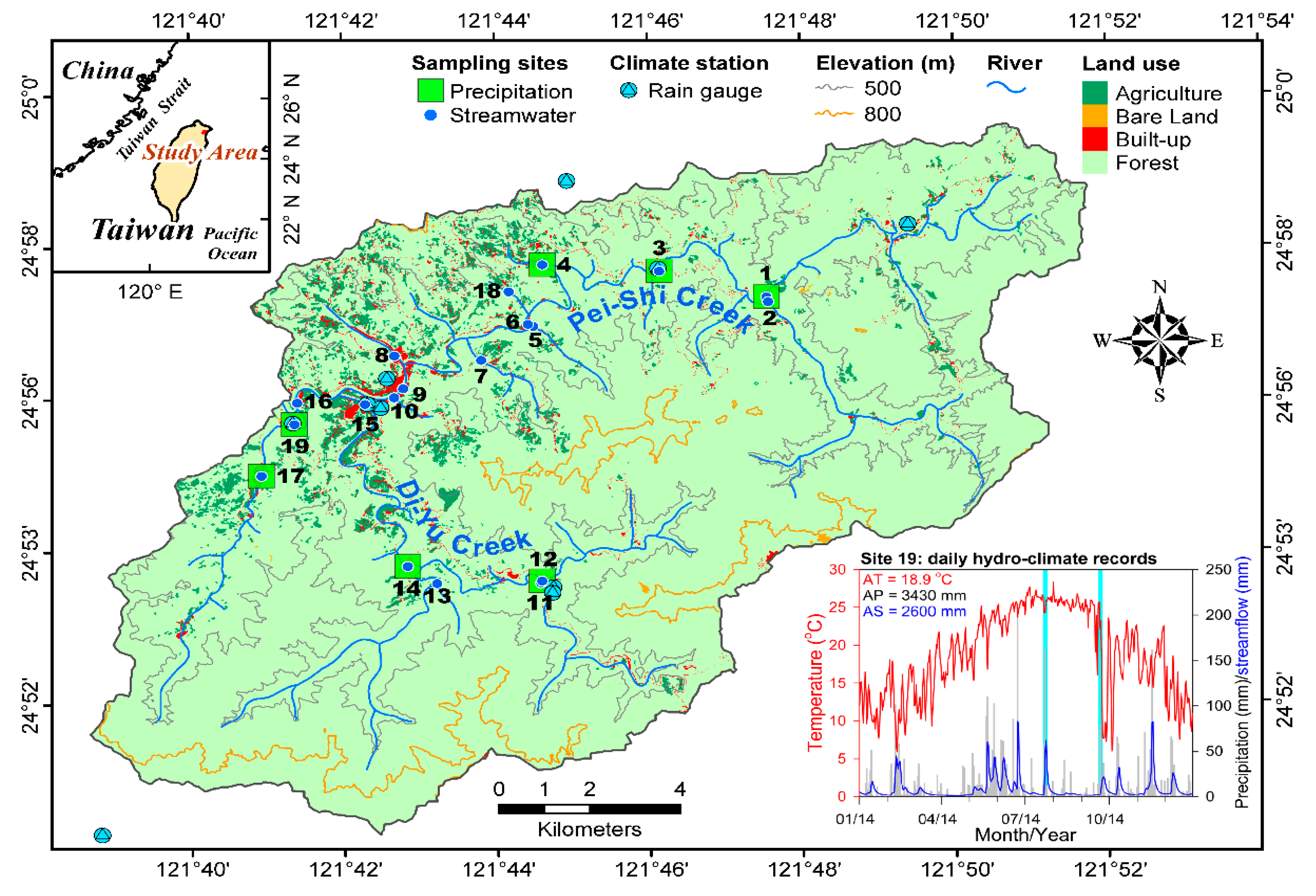
2.1. Study Sites

This study was conducted in Feitsui Reservoir Watershed (FRW) in northeastern Taiwan, which is the main domestic water supply for the mega city, Taipei (Figure 1). Totally, 7 precipitation sites and 19 stream water sites were deployed along the Pei-Shi Creek and the Di-Yu Creek, two main upstream tributaries of the reservoir watershed. The annual mean temperature of the region is 18.9 °C, with monthly temperature ranging from 12.5 (January) to 26.5 °C (July) (Figure 1). The high mean annual precipitation of 3770 mm, with 68% taking place between May and September [30,31], is also highly variable spatially, increasing from 3500 mm in the southwestern part of the FRW to 5000 mm in the northeastern of the FRW during 2001–2010 due to the mountainous landscape. Typhoons, which mainly occur in summer and autumn, usually bring large amounts of precipitation in a few days. In the winter, the northeast monsoons could also bring substantial but more gentle rainfall. During the study period (2014), two typhoons made landfall to Taiwan: typhoon Matmo on 22–23 July and typhoon Fong-Wong on 20–22 September. The weekly precipitation (streamflow) associated with the two typhoon-affected weeks was 250 (200) mm and 180 (130) mm, respectively, based on the record of watershed 19 (Figure 1). One strong thunderstorm event from 22 to 26 June also poured down 270 (140) mm of precipitation (streamflow) (Figure 1). During the winter monsoon period (December to February), there were 10 weeks with a weekly precipitation greater than 50 mm, showing the abundant winter precipitation in the region. Long-term observation that takes inter-annual climate variation into consideration is desirable, but it is difficult to carry out for multiple sites without institutional long-standing support, especially in mountainous regions. The number of typhoons, precipitation, and temperature were not atypical compared to the records from the past two decades (Figure S1).
The elevation of FRW ranges from 180 to 1127 m, with a mean slope steepness of 42%. The dominant soils are Entisols and Inceptisols, with high silt contents developed from argillite and slate with sandstone interbeds [32]. The land use types within the FRW mainly include forests (84%), agricultural lands (8.2%), and other built-up areas (7.7%) [33]. The natural secondary forests are dominated by species of Fagaceae and Lauraceae, including Persea thunbergii (Sieb and Zucc.) kosterm, Castanopsis uraiana (Hayata) Kanehira and Hatusima, Cryptocarya chinensis (Hance) Hemsl., and Araliaceae such as Schefflera octophylla (Lour.) Harms [34,35]. The agricultural activities are restricted to pre-existing farmlands because the region was designated for water resource protection following the construction of the Feitsui Reservoir in 1987. Tea plantations (approx. 1200 ha) dominate the agriculture land, and the fertilizer applications can reach 786 kg-N ha−1 yr−1 [27]. The drainage area of the 19 watersheds varying from 1.4 (site 18) to 195.4 km2 (site 16) presents a wide range of proportions of different land use types, with agricultural land ranging from 0.2% (site 13) to 22.1% (site 4) (Figure 1 and Table 1).

2.2. Water Collections and Chemical Analysis

From January 2014 to December 2014, bulk precipitation and stream water were collected weekly (Figure 1 and Table 1). The bulk precipitation samples were collected with a 20 cm-diameter polyethylene (PE) bucket (approx. 10 L), while the stream water samples were taken by plunging a 1-L PE bucket into the stream. For both precipitation and stream water, a subsample (approx. 600 mL) of water was taken to measure the pH and conductivity in situ; the rest was filtered with a 0.45 µm filter. A 100 mL filtrate was reserved within a PE bottle and transported to the laboratory in the National Taiwan University in Taipei. The filtered samples were kept at 4 °C in a refrigerator without any chemical preservatives before chemical analysis. The concentrations of major cations (Na+, K+, Mg2+, Ca2+, NH4+) and anions (Cl, NO3, SO42−) were analyzed by ion chromatography via Dionex ICS-1100 (Thermo Fisher Scientific Inc.®, Sunnyvale, CA, USA) and Methrom® 886 basic plus (Methrom®, Herisau, Switzerland). The concentration of PO43− was measured using the standard vitamin C-molybdenum blue method with the detection limit of 0.01 μM [36]. Because the concentrations of NH4+ and PO43− were below the detection limits for more than 75% of the precipitation and stream samples, they were excluded from subsequent analyses.

2.3. Precipitation Estimation and Stream Flow Simulation

In FRW, there are in total 10 meteorological stations; five are maintained by the Water Resource Agency (WRA) and the other five are maintained by the Central Weather Bureau (CWB) of Taiwan (Figure 1). The daily evaporation data were provided by the Taipei Feitsui Reservoir Administration (TFRA) and the station is located at the dam of the reservoir. The areal rainfall pattern over the study area was interpolated by the Thiessen polygon approach to present the spatial variation, from which the precipitation for individual watersheds can be derived from these weekly spatial rainfall distributions. The records of discharge were provided by the TFRA, and the inflow discharge is summed in the records from two main creeks nearby sites 16 and 19 (Figure 1). Thus, the streamflow of the ungauged watersheds was simulated via a conceptual topographic-based hydrological model, topmodel [37,38,39], using the R package dynatopmodel Ver. 1.2.1 [39]. The topmodel was used to simulate the daily streamflow considering the daily rainfall, daily evaporation, and terrain data obtained from ALOS World 3D-30m (Ver. 2.1) [40]. The observed daily streamflow was utilized to train the best parameter set to fit low, normal, and extreme values of simulated flow particularly, and the criterion of best parameters was selected based on the Kling–Gupta efficiency (KGE), where the closer a value is to unity the better [41,42]. The simulation performed well (KGE = 0.88) and the parameter set (Table S1) was applied to all watersheds, but employing their own climatic inputs and terrain information to simulate their daily streamflow. The annual runoff ratio (estimated streamflow/precipitation) of all the watersheds ranged from 0.70 to 0.80, which was consistent with our previous estimation [5]. The paired weekly ion concentrations and water quantity of precipitation and streamflow were used to calculate the precipitation input, stream water output, and nutrient input-output budgets (stream water output−precipitation input).

2.4. Statistical Nutrient Budget Model

In this study, the widely used rating curve method (power-law regression between nutrient export and stream discharge) was used to estimate the nutrient export (Equations (1) to (8)). The constant in the rating curve is relevant to the nutrient source and represents the basal export, as the stream discharge is zero. Although it cannot perfectly explain the nutrient export at zero stream discharge, it would not be the case for perennial streams. The exponent coefficient is also relevant to the source, but it responds to the change in the stream discharge. Conceptually, a coefficient greater than one indicates that the discharge accelerates the nutrient export, which is often referred to as “enhancement”, with sediment transport as a typical example. A coefficient that is close to one presents that the nutrient export linearly increases with stream discharge. In this case, it often implies that the nutrient source is abundant. A coefficient smaller than one represents that the nutrient has a limited source, so that the rate of nutrient export decreases as the stream discharge increases, which is also termed “dilution” [19]. We established regression models of the input-output nutrient budgets in which the agricultural land cover, discharge, and atmospheric inputs are regarded as source-associated factors and are then incorporated to determine their contribution to stream nutrient export [19,43,44,45]. Five independent variables were included in the regression models—i.e., the fraction of agricultural land cover (AgrFrac) of each watershed (from 0.2 to 22.1 here, Table 1), the weekly discharge (Q, mm w−1), the weekly precipitation input for analyzed ion i (Inputi, kg ha−1 w−1), and topographical slope and elevation. Different multiple power-law regressions with various combinations of nutrient input, runoff, AgrFrac, slope, and elevation were examined to evaluate their predictability in nutrient budgets [7,46,47,48]. Eight settings of multiple regressions are used in this study (Equations (1)–(8)):
Model   1 :   y i = a + b × Q c × A g r F r a c ,
Model   2 :   y i = a + b × Q A g r F r a c + d × I n p u t i ,
Model   3 :   y i = b × Q c × A g r F r a c + d × I n p u t i ,
Model   4 :   y i = a + b × Q c × A g r F r a c + d × I n p u t i ,
Model   5 :   y i = a + b × Q c × A g r F r a c × S L O P E + d × I n p u t i ,
Model   6 :   y i = a + b × S L O P E × Q c × A g r F r a c + d × I n p u t i ,
Model   7 :   y i = a + b × Q c × A g r F r a c × E l e v + d × I n p u t i ,
Model   8 :   y i = a + b × E l e v × Q c × A g r F r a c + d × I n p u t i ,
where yi is the weekly modeled or estimated nutrient budget (kg ha−1 w−1) for ion species i, and Q, AgrFrac, and Inputi stand for weekly discharge (mm w−1), the fraction of agricultural land cover, and the precipitation input for species i (kg ha−1 w−1), respectively. The SLOPE and Elev are average values of slope (%) and elevation (m) for watersheds. The coefficients (a, b, c, and d) were parameters determined through performance measures. The weekly nutrient data derived from 12 of 19 watersheds across a wide range of proportions of agricultural land cover (AgrFrac ranging from 0.2 to 22.1) were used to establish the regression models, while the data of the other 7 watersheds (AgrFrac ranging from 1.0 to 18.9) were utilized to validate the models (Table 1). The Akaike Information Criterion (AIC) was applied to select the best model from several alternative models, in which the model with the lowest AIC is the most cost-effective [49,50]. The calculation of AIC can be expressed as Equation (9):
AIC = 2 log ( m ) 2 n ,
where m is the maximum likelihood and n is the number of parameters in the model. The model performance between the predicted and observed values was evaluated by the coefficient of determination (R2) and the Nash–Sutcliffe efficiency (NSE), in which the closer a value is to unity, the better the model will be. The residual (i.e., the difference between the predicted and observed values) was evaluated by the root mean square error (RMSE) [51,52].

3. Results

3.1. Nutrient Concentrations and Fluxes

The mean annual volume-weighted mean (VWM) pH (calculated from the annual VWM H+ concentration) of the seven bulk precipitation sites ranged from 4.64 to 5.05, which was significantly lower than the mean annual VWM pH of the stream water of the 19 sites, ranging from 6.69 to 7.27 (p < 0.01, Figure 2 and Table S2). The VWM ion concentrations of stream water were considerably higher than those of precipitation for all ions except K+, which were not significantly different between precipitation and stream water (Figure 2). The VWM concentrations of Na+ and Cl, the most abundant ions in sea salts, were 180–266 and 100–198 µeq L−1, respectively, in stream water, and were more than two times higher than those in precipitation, 73–102 and 74–108 µeq L−1 (Figure 2 and Table S2). The annual VWM concentrations of Mg2+ and Ca2+ were more than five times higher in stream water than in precipitation. The SO42− concentration in stream water was approximately 2–4 times of that in precipitation (Table S2). The annual VWM concentrations of NO3 in the stream water of watersheds with a forested land cover greater than 94% (23.7–25.5 µeq L−1) were similar to the concentrations in precipitation (19.7–25.2 µeq L−1), but the concentrations in the stream water of watersheds with a non-forested land cover of 5.3% (site 19, 29.9 µeq L−1) and 22.1% (site 4, 214.3 µeq L−1) were elevated to 1.7- and 8-fold higher than those in precipitation (18.0 µeq L−1 in site 19 and 26.2 µeq L−1 in site 4) (Figure 2 and Table S2). In addition, there was a trend of decrease from northeastern sites to southwestern sites in the concentrations of Na+, K+, Cl, and Mg2+ in precipitation, whereas the Ca2+, NO3, and SO42− did not have such a spatial pattern (Figure 1 and Table S2). The patterns of annual ion fluxes in precipitation and stream water were similar to the patterns of ion concentrations described above (Tables S2 and S3).

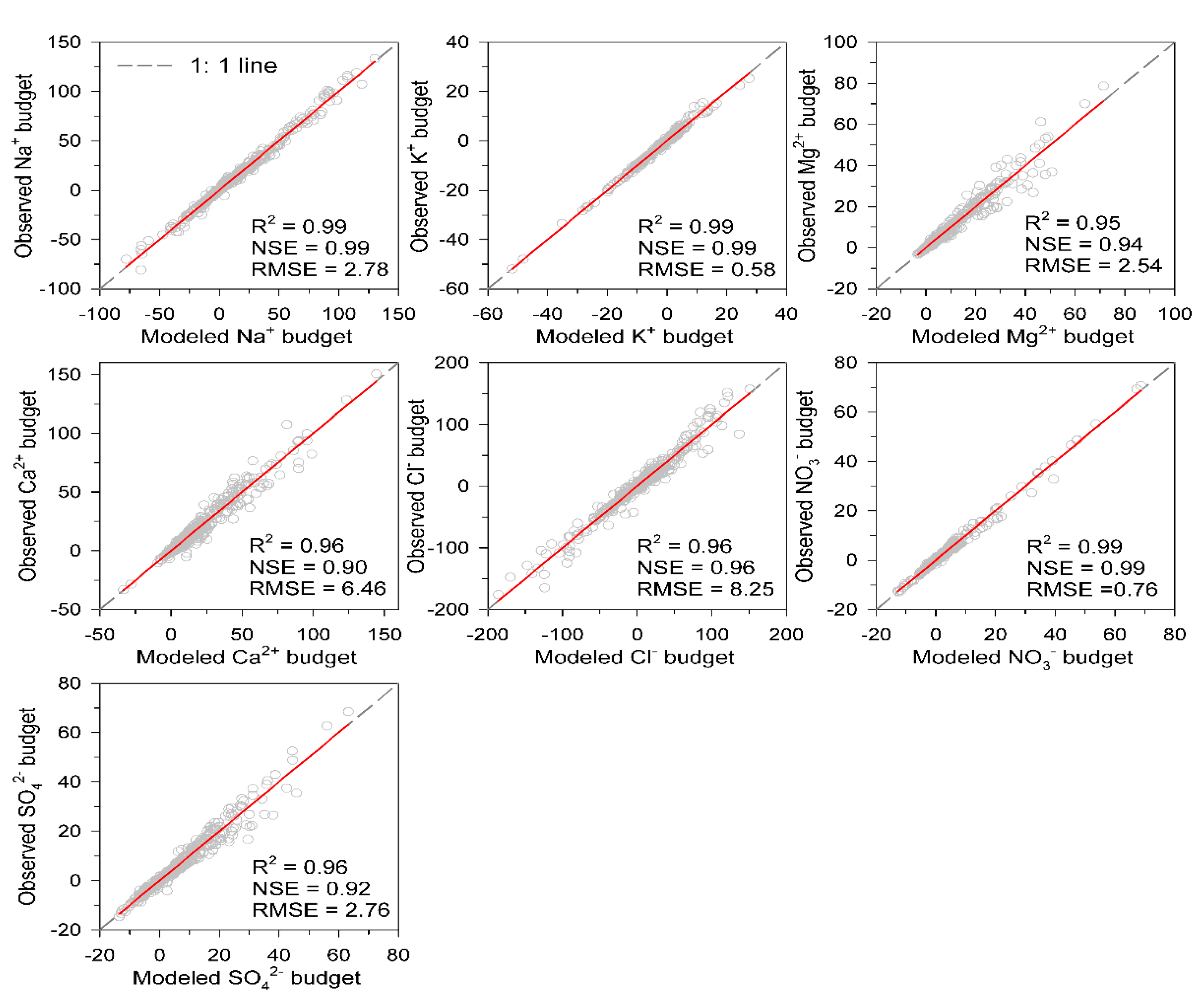
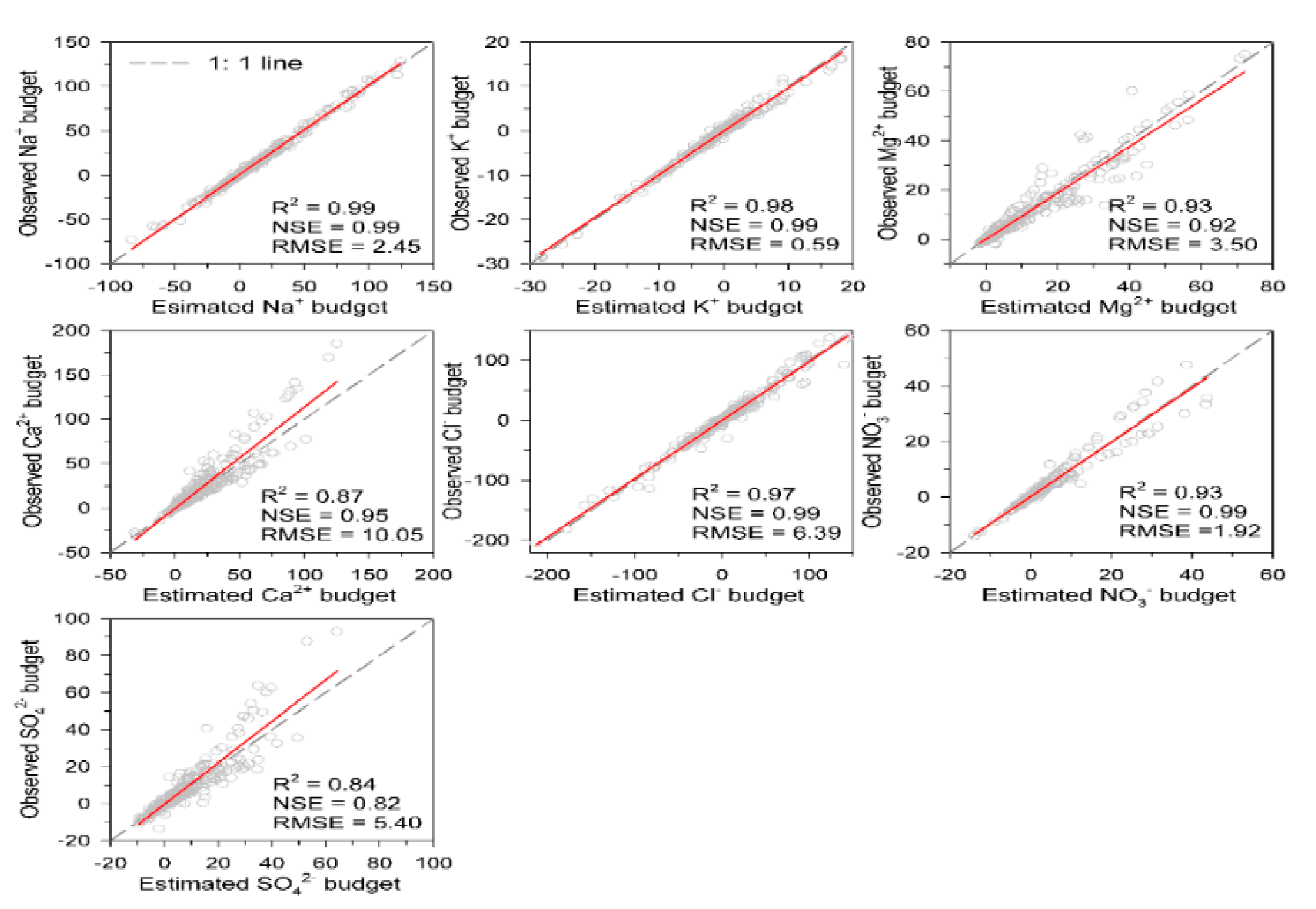
3.2. The Nutrient Budget Simulation
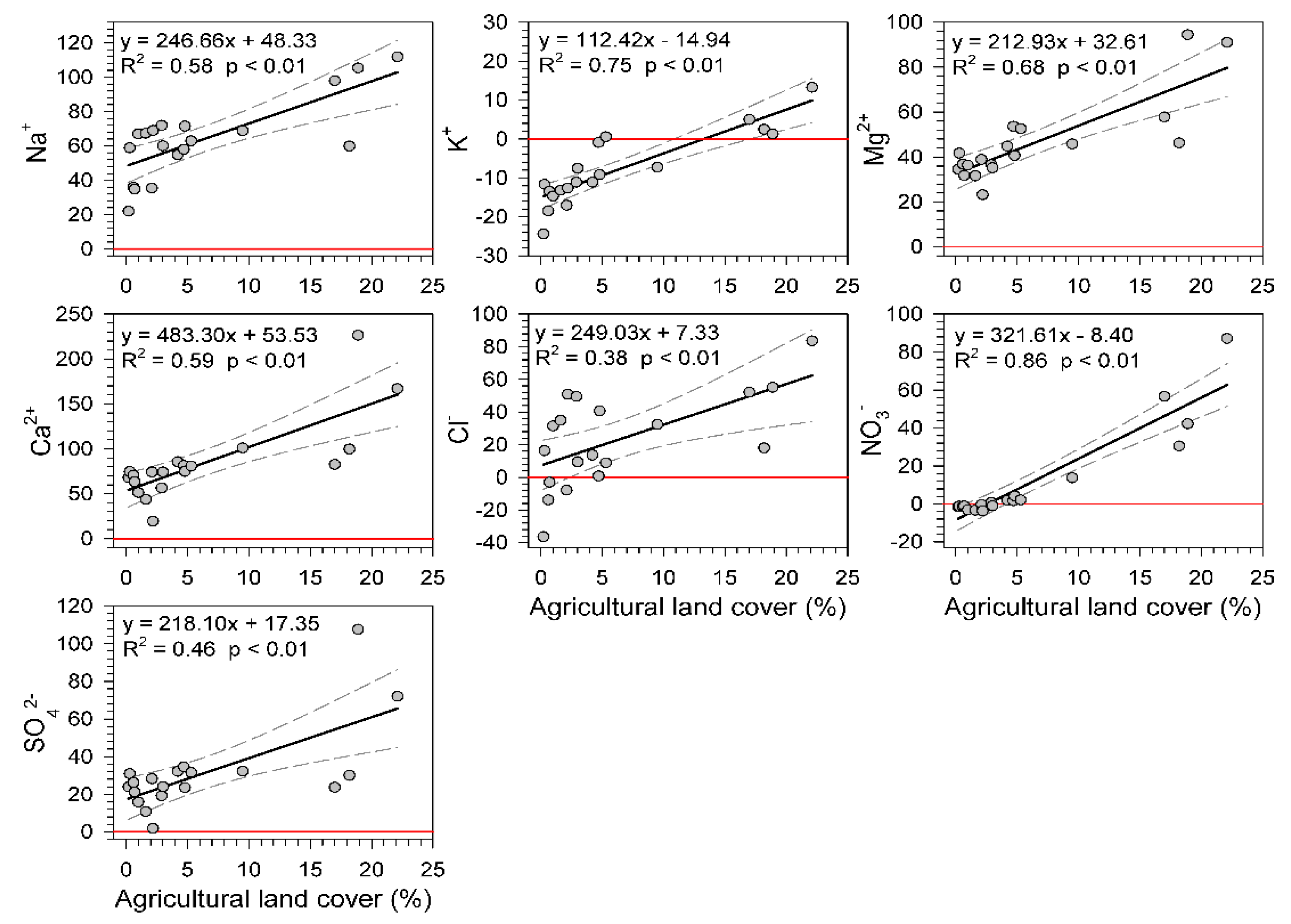
At an annual scale, the relationships between agricultural land cover (%) and annual nutrient budgets were significant (p < 0.01) for all ions with Na+ (R2 = 0.58), K+ (R2 = 0.75), Mg2+ (R2 = 0.68), Ca2+ (R2 = 0.59), Cl (R2 = 0.38), NO3 (R2 = 0.86), and SO42− (R2 = 0.46) (Figure 3). The annual discharge was also highly correlated with the annual nutrient budgets for Na+ (R2 = 0.73, p < 0.01), Cl (R2 = 0.79, p < 0.01), and NO3 (R2 = 0.24, p = 0.035), but not for K+, Mg2+, Ca2+, and SO42− (data not shown). The average elevation of the watershed was only significantly related to the Na+ (R2 = 0.49, p < 0.01) and Cl (R2 = 0.42, p < 0.01), whereas the average slope of the watershed was not significantly related to any of the annual budgets (data not shown).
However, the relationships between nutrient budget with discharge and agricultural land cover for ions were diverse at weekly scale. Based upon the various settings of multiple power-low equations and AICs, we tried to identify the best fit model using the data of 12 watersheds (Table 1). The results showed that “Model 4”, which simultaneously took precipitation input, discharge, and agricultural land cover into account, had the most satisfactory performances for Na+, K+, Cl, and NO3, as indicated by the lowest AICs (Table 2). For Model 4, the R2 (NSE, RMSE) of data fitting between the weekly observed budgets against the modeled budgets ranged from 0.96 (0.96, 8.25) for Cl to 0.99 (0.99, 0.58) for K+, respectively. While Model 6, which also includes slope as a predictor, in addition to three variables in Model 4, performs the best for Mg2+, Ca2+, and SO42−, with the lowest AICs (Table 2), and with the R2 (NSE, RMSE) ranging from 0.95 (0.94, 2.54) for Mg2+ to 0.96 (0.90, 6.46) for Ca2+, respectively. Adding elevation as an additional predictor (i.e., Models 7 and 8) does not improve the predictive power of estimating nutrient budgets (Table 2). All the regressed lines paralleled with 1:1 lines (Figure 4) indicated that the simulations from the models were unbiased. For the validation using data of the other seven watersheds (Table 1), the R2 (NSE, RMSE) between the weekly estimated budgets against the observed budgets varied from 0.84 (0.82, 5.40) for SO42− to 0.99 (0.99, 2.45) for Na+ (Figure 5). The interception of fitting models ranged from −0.789 for Cl to 0.119 for Mg2+. The coefficients c in the fitting models, between discharge (Q) and the fraction of agriculture (AgrFrac), indicating the strength of the interactive effects between Q and AgrFrac on nutrient export, ranged from 0.991 for Na+ to 4.491 for K+ and 10.245 for NO3 (Table 3). The coefficients d of precipitation input, standing for the contribution of precipitation to the nutrient budget estimation, varied from −0.961 for Ca2+ to −1.016 for SO42− (Table 3). Furthermore, the exports of Cl, Mg2+, Ca2+, and SO42− could be estimated promisingly by Model 1 (considering the discharge and fraction of agriculture, Table 3), and the performances increase slightly from Model 1 to Model 4. The export estimations of Na+ and K+ based on Models 2–4 (R2 > 0.90) are much better than those of Model 1 without considering the precipitation input (R2 < 0.30, Table 2).

4. Discussion

4.1. Characteristics of Precipitation and Stream Water Chemistry

The annual VWM pH between precipitation and stream water showed a striking difference across all sites, in which the precipitation annual VWM pH was consistently less than 5.0 (the criterion for acid rain), while the minimal annual VWM pH of stream water was 6.69, with 13 of the 19 sites > 7.0 (Figure 2 and Table S2). This result was consistent with that at the Fushan Experimental Forest (FEF), a forested watershed 20 km southwest of the FRW. The long-term monitoring (1994–2013) at the FEF revealed that about 90% of the annual VWM pH of precipitation was lower than 5.0, but there was no sign of acidification in stream water with a 20-year annual VWM pH of 6.95 [4]. We had no measurements of groundwater across various watersheds, so we did not include it in the estimation of the nutrient budgets. The input from groundwater with a higher concentration of base cations, such as Na+, Ca2+, and Mg2+, was believed to play a critical role in neutralizing the acidity in the FEF [4,53], and likely also in our study sites (Figure 2). In many temperate forests, the acidification of stream water was usually followed by the acidification of precipitation [1,54]. However, the divergence of the precipitation and stream water acidity in this subtropical region was strikingly different from those in temperate forests. The high rainfall accompanies a higher concentration of ions such as SO42− and NO3, leading to high acidic depositions, which are comparable as findings in FEF and are higher than in most forests worldwide [55]. In spite of there continuously being a high deposition of sulfates and nitrates in Asia and Taiwan [26], there is no sign of harmful effects on the ecosystem structure and function except in China [56]. However, the Ca2+ deposition in FEF showed a significant declining trend over the past 20 years, indicating that the soils could be further acidified and that the effects on the ecosystem remain a critical concern [55]. The ratio of Cl/Na+ was 1.05 in precipitation, which was close to 1.1 in sea water, indicating that the composition of Na+ and Cl did not change significantly during the aerosol formation and transportation before the collection of the deposition [57,58]. However, the ratio of Cl/Na+ in stream water decreased to lower than 0.80 because the enhancement of the Na+ concentration in stream water was approximately 50% higher than that of Cl (Table S2), which was attributed to the deep chemical weathering [59].
The differences in nutrient export between disturbed and forested watersheds were most evident for K+ and NO3, ions associated with fertilizers, which were approximately three and eight times higher, respectively, in watershed 4 than in watershed 13 (Table S3). The relationships between the annual nutrient budgets and agricultural land cover also revealed that when the agricultural land cover was higher than 5%, the net export of K+ and NO3 was be remarkably increased (Figure 3). A study that examined the effects of land cover on the sediment regime in the Upper Little Tennessee River a with gentle slope (5%) in North Carolina showed that the disturbed sites with >10% of non-forested land cover would have 5- to 9-fold more suspended sediment and bedload transport than less disturbed sites (<3% of non-forested land cover) [60]. A study in the coastal plain watersheds surrounding Chesappeake Bay also suggested that the nitrate concentrations of the stream water significantly increased when the non-forested land cover was higher than 10% [44]. In our study region (FRW) with a slope steepness of 42%, the hydrochemical responses are likely more sensitive to subtle conversion from forested to non-forested land cover, because a larger slope steepness will enhance erosion [26]. Many studies have indicated that water quantity (precipitation or streamflow) exerts a strong control on the export and budget of major ions—i.e., the precipitation control or hydrological control—and not just nitrogen in undisturbed forest watersheds [4,61,62]. Our study showed that, in watersheds disturbed by anthropogenic activities, the agricultural land cover is probably an even more important factor that contributes to the elevation of the concentration and flux of most ions (Figure 3).

4.2. Indications from the Nutrient Budgets Estimations

Land cover change, especially the conversion of natural forest to cropland and urban land use, is a critical issue for soil-water resource stabilization worldwide [25,63]. The issue is more urgent in humid tropical/subtropical mountainous regions, such as Taiwan, where the plentiful rainfall, at an annual average of 2500 mm, together with the rough topography control the soil erosion and nutrient budgets [4,64]. Previous studies conducted in steep-slope watersheds in Taiwan and South Korea have suggested that the sediments and nutrient exports, such as total nitrogen and total phosphorous, could be fitted well with discharge (R2 > 0.8) using a logarithm- or exponent-type regression model [65,66]. We further considered the interaction between discharge and the agricultural land cover as a proportion of the watershed area and atmospheric input across 19 watersheds, which significantly improved the accuracy of the nutrient budget estimation (R2 > 0.9).
Our power-law regressions presented the different levels of incorporation of three parameters—precipitation input, discharge, and fraction of agricultural land (AgrFrac)—in nutrient budgets. The estimations of Cl, Mg2+, Ca2+, and SO42− budgets can perform well using Model 1 (considering discharge and AgrFrac), and the performances increase slightly from Model 1 to Model 4 (considering precipitation input, discharge, and AgrFrac). Because the Cl is the conservative trace and there is no significant evaporite in this region [67], the satisfactory estimations of Cl from Model 1 to Model 4 indicate that the transport of Cl from precipitation to streamflow is relatively unreactive in ecosystems under a high Cl deposition, as in our study region [68]. The coefficient b of the discharge term, which is lower than unity, showed a significant dilution effect during chloride transport (because the AgrFrac must be less than one). In contrast to chloride, the other three ions (Mg2+, Ca2+, and SO42−) showed some improvement from Model 1 to Model 4 (including precipitation input into estimation), indicating that the AgrFrac within watersheds is a first control on the ion export, but the atmospheric input acted as a secondary control. For Na+ and K+, the estimations of Models 2–4 considering precipitation input, discharge, and AgrFrac with different settings (R2 > 0.90) are much better than those of Model 1 (R2 < 0.30, Table 2), demonstrating that the two ion exports require taking atmospheric input into account. Even so, there are still some differences between the two export behaviors. The Na+ export, in fact, is quite similar to that of Cl in terms of the exponent coefficient, likely because sea salt is also the main Na+ source. Another main source of sodium is silicate weathering and fertilizer, and therefore its export is more complicated than that of chloride. Comparing to Na+, the K+ export is more significantly regulated by AgrFrac. The higher coefficient c of exponent between discharge and AgrFrac presents the magnitude of hydrologic control (Table 3). For NO3 export, it is the only ion which necessitates taking the enhancement effect into account (Table 3) [5,45,69]. The higher agricultural land cover could enhance the hydrologic control significantly under the same exponent coefficient, according to Model 4 (Table 3). The higher coefficient, such as 4.491 in K+ and 10.245 in NO3, indicated that the potassium and nitrate would be transported more dramatically than the other ions (Table 3). The highest exponent coefficient connected discharge with AgrFrac in nitrate, and also implied that fertilizer application could have dominant effects on the net export of nitrate from watersheds. A study conducted on watersheds along Lanyang-Shi in northeastern Taiwan indicated that the dissolved inorganic nitrogen (DIN) deposition likely led to a high background yield, and agricultural activity within the watershed could account for 49% of the DIN export [70]. Our result is similar to that when both the precipitation input and agricultural land cover are considered for comprehending the input-output budget of nitrogen. The effects will be likely exaggerated when the amount of fertilizer applied exceeds the watershed retention capacity. If the > 700 kg-N ha−1 yr−1 application of N-fertilizers reported previously is common in the FRW [27], it would be 3.5 times that of the maximum global nitrogen application rate, 200 kg-N ha−1 yr−1 [71,72], and is likely way more than is required for plant growth. It can be expected that the excessively added nitrogen will be rapidly flushed out with runoff, especially in regions with abundant rainfall, such as our study area. Other geographical factors, such as elevation and slope, could be important factors in nutrient export if the study is conducted on a global or continental scale. From our results, the performance of regression models shows some improvement in estimating the nutrient budgets of Mg2+, Ca2+, and SO42, but not for Na+, K+, Cl, and NO3 when the slope was also included to the model in addition to the discharge, fraction of agricultural land cover, and precipitation input (i.e., Model 6 in Table 2 and Table 3). Adding elevation to the models (Models 7 to 8 in Table 2) did not improve the models’ performance in estimating the nutrient budgets. The limited effects of slope and no effect of elevation in estimating the nutrient budgets are possibly because the slope (31–45%) and elevation (484–647 m) do not vary much among the 19 watersheds in a mountainous region spanning over a few kilometers, which minimizes their effects on modeling nutrient exports (Table 1).
The higher annual net budgets (net export) of base cations of Na+, Ca2+, and Mg2+ likely indicated that the rapid chemical weathering could provide a great quantity of these cations [59,67]. Chemical weathering that dissolves rock into ions is crucial for soil production and acidity mitigation and is strongly accelerated by runoff and physical erosion, and thus it prevails in wet young mountain environments [67,73]. The long-term observation in the FEF near to FRW revealed that both the higher pH and base cation concentrations in stream water were attributed to the high contribution of groundwater to the streamflow and the continuous exchange of cations between the groundwater and stream water [4]. The considerable net export of base cations during heavy rainfall events can be also found in the Leinhuachi and Fushan Experimental forest in central and northern Taiwan [4,74], and in Liwu and Beishi river in eastern and northern Taiwan [59,67]. These results suggested that these extreme events such as typhoons and thunderstorms had a great contribution to annual exports of base cations. Agricultural practices exposed fresh soil, and the application of nitrogenous fertilizers promoted acidity generation, which both accelerated weathering and increased the base cation export into stream water. The elevated erosion rates will deplete the soil productivity and may also generate an extra carbon source and consequent eutrophication downstream [75,76]. Our analysis of 19 watersheds from one complete year reveals several important insights into the estimation of various nutrient budgets, comprising atmospheric deposition, discharge, and agricultural land cover, yet it does not take inter-annual variations into consideration. Thus, extrapolating the result to the long-term situation needs to be done with caution. Although it is challenging to take long-term measurements for many years, efforts are strongly encouraged whenever possible, as such efforts, even rare ones, are highly valuable. Despite the unclear internal processes within watersheds, our nutrient budget approach based upon a series of watersheds provides the preliminary assessment to evaluate the impacts of agriculture and atmospheric deposition on water quality, which will be helpful for water resource management.

5. Conclusions

The dynamics of nutrient budget—the difference between output via stream water and input via precipitation—reveal the overall outcomes of interactive effects between internal ecosystem process and external environmental forces. It is critical to confirm the key control affecting water quality under a rapidly shifting climate and land cover change. Our simple series of regression models revealed that the weekly nutrient budget can be well estimated considering discharge, agricultural land cover, atmospheric inputs, and slope simultaneously (R2 ≥ 0.95), yet the effects of these variables on the nutrient budgets varied among different ions. The role of atmospheric input of Cl, Mg2+, Ca2+, and SO42− in the nutrient budget is minor. The slope of the watershed has some improvement on simulations of nutrient budgets of Mg2+, Ca2+, and SO42−, but not for those of Na+, K+, Cl, and NO3. The role of the atmospheric input of Cl, Mg2+, Ca2+, and SO42− in nutrient budget is minor. Furthermore, the incorporation of atmospheric Na+ and K+ inputs is indispensable for accurately estimating the corresponding riverine exports, since the sources of Na+ and K+ are in part from sea salt, except for provisioning abundantly from the watershed. The NO3 budget presents a strong interplay with the atmospheric input and agricultural land. Moreover, the large coefficient (10.2) in the exponent term between discharge and the fraction of agricultural land cover for the NO3 export indicates that NO3 is the strongly hydrologically controlled. Due to the difficulty of sampling 19 watersheds for multiple years, our result is based on one complete year of data, without including inter-annual variation in the analysis, and so extrapolating the result to infer long-term patterns needs to be done with caution. Although the internal processes within watersheds are still not clear, our nutrient budget approach based upon a series of watersheds provides the preliminary calculation to assess the impacts of agriculture and atmospheric deposition on water quality, suggesting that strategies of both fertilizer reduction and emission control are effective ways to improve water quality and mitigate eutrophication. If projections of future interactions between climate change and land uses are available, they would provide an opportunity to realize the biogeochemical processes of the terrestrial ecosystem under different warming scenarios [77,78].

Supplementary Materials

The following are available online at https://www.mdpi.com/2073-4441/12/10/2800/s1: Table S1: Input parameters in Hydrological Response Unit (HRU); Table S2: The estimated annual water quantity (mm), observed volume-weighted mean (VWM) pH and concentrations (µeq L−1) of major elements in precipitation and streamwater measured in 2014 across 19 watersheds; Table S3: The annual total fluxes of precipitation input and stream water output of major elements in 2014 across 19 watersheds. Figure S1. The annual typhoon occurrence (a), annual mean temperature and annual precipitation (b) during the period 2001–2019 based on data from the climate station of C0A530 maintained by Central Weather Bureau (between sites number 8 and number 9) in Figure 1. The typhoon occurrence was defined as those which were < 100 km in distance from the study region to their paths at the closest (Tu et al., 2009). Figure S2: The daily hydro-climate data of 18 watersheds in 2014 except for number 19 in Figure 1. The AT, AP, and AS indicate the annual mean temperature, annual precipitation, and annual streamflow, respectively.

Author Contributions

Conceptualization, C.-T.C. and J.-C.H.; methodology, C.-T.C. and J.-C.H.; software, Y.-T.S.; formal analysis, C.-T.C., Y.-T.S., L.-C.L., J.-Y.L., and T.-Y.L.; data curation, C.-T.C., Y.-T.S., L.-C.L., J.-Y.L., T.-Y.L., and J.-C.H.; writing—original draft preparation, C.-T.C., T.-C.L., and J.-C.H.; writing—review and editing, C.-T.C., T.-C.L., and J.-C.H.; Supervision and funding acquisition, J.-C.H. All authors have read and agreed to the published version of the manuscript.

Funding

This research was funded by Ministry of Science and Technology and NTU Research Center for Future Earth to J.C. Huang (MOST 107-2621-B-002-003-MY3 and 107L901004), and C.T. Chang (MOST 105-2410-H-029-056-MY3, 108-2313-B-029-001 and 109-2621-B-029-004).

Acknowledgments

We thank for the assistant and students for the field work and laboratory analysis.

Conflicts of Interest

The authors declare no conflict of interest.

References

  1. Likens, G.E.; Bormann, F.H. Biogeochemistry of a Forested Ecosystem, 2nd ed.; Springer: New York, NY, USA, 1995. [Google Scholar]
  2. Padowski, J.C.; Gorelick, S.M. Corrigendum: Global Analysis of Urban Surface Water Quality Supply Vulnerability. Environ. Res. Lett. 2014, 9, 119501. [Google Scholar] [CrossRef]
  3. Kaushal, S.S.; Groffman, P.M.; Band, L.E.; Shields, C.A.; Morgan, R.P.; Palmer, M.A.; Belt, K.T.; Swan, C.; Findlay, S.E.G.; Fisher, G.T. Interaction between Urbanization and Climate Variability Amplifies Watershed Nitrate Export in Maryland. Environ. Sci. Technol. 2008, 42, 5872–5878. [Google Scholar] [CrossRef] [PubMed]
  4. Chang, C.-T.; Wang, L.-J.; Huang, J.-C.; Liu, C.-P.; Wang, C.-P.; Lin, N.-H.; Wang, L.; Lin, T.-C. Precipitation controls on nutrient budgets in subtropical and tropical forests and the implications under changing climate. Adv. Water Resour. 2017, 103, 44–50. [Google Scholar] [CrossRef] [Green Version]
  5. Chang, C.-T.; Huang, J.-C.; Wang, L.; Shih, Y.-T.; Lin, T.-C. Shifts in stream hydrochemistry in responses to typhoon and non-typhoon precipitation. Biogeosciences 2018, 15, 2379–2391. [Google Scholar] [CrossRef] [Green Version]
  6. Huang, J.-C.; Kao, S.-J.; Lin, C.-Y.; Chang, P.-L.; Lee, T.-Y.; Li, M.-H. Effect of subsampling tropical cyclone rainfall on flood hydrograph response in a subtropical mountainous catchment. J. Hydrol. 2011, 409, 248–261. [Google Scholar] [CrossRef]
  7. Rankinen, K.; Keinänen, H.; Bernal, J.E.C. Influence of climate and land use changes on nutrient fluxes from Finnish rivers to the Baltic Sea. Agric. Ecosyst. Environ. 2016, 216, 100–115. [Google Scholar] [CrossRef]
  8. Palmer, S.M.; Driscoll, C.T.; Johnson, C.E. Long-term trends in soil solution and stream water chemistry at the Hubbard Brook Experimental Forest: Relationship with landscape position. Biogeochemistry 2004, 68, 51–70. [Google Scholar] [CrossRef]
  9. Likens, G.E. Biogeochemistry of a Forested Ecosystem; Springer Science and Business Media LLC: Berlin/Heidelberg, Germany, 2013. [Google Scholar]
  10. Bobbink, R.; Hicks, K.; Galloway, J.N.; Spranger, T.; Alkemade, R.; Ashmore, M.; Bustamante, M.M.C.; Cinderby, S.; Davidson, E.A.; Dentener, F.; et al. Global assessment of nitrogen deposition effects on terrestrial plant diversity: A synthesis. Ecol. Appl. 2010, 20, 30–59. [Google Scholar] [CrossRef] [Green Version]
  11. Runyan, C.W.; D’Odorico, P.; Vandecar, K.L.; Das, R.; Schmook, B.; Lawrence, D. Positive Feedbacks Between Phosphorous Deposition and Forest Canopy Trapping Evidence from Southern Mexico. J. Geophy. Res. Biogeosci. 2013, 118, 1521–1531. [Google Scholar] [CrossRef]
  12. Likens, G.; Driscoll, C.T.; Buso, D.; Siccama, T.; Johnson, C.E.; Lovett, G.M.; Ryan, D.; Fahey, T.; Reiners, W. The biogeochemistry of potassium at Hubbard Brook. Biogeochemistry 1994, 25, 61–125. [Google Scholar] [CrossRef]
  13. Lovett, G.M.; Likens, G.E.; Buso, D.C.; Driscoll, C.T.; Bailey, S.W. The biogeochemistry of chlorine at Hubbard Brook, New Hampshire, USA. Biogeochemistry 2005, 72, 191–232. [Google Scholar] [CrossRef]
  14. Driscoll, C.T.; Lawrence, G.B.; Bulger, A.J.; Butler, T.J.; Cronan, C.S.; Eagar, C.; Lambert, K.; Likens, G.E.; Stoddard, J.L.; Weathers, K.C. Acidic Deposition in the Northeastern United States: Sources and Inputs, Ecosystem Effects, and Management Strategies. Bioscience 2001, 51, 180–198. [Google Scholar] [CrossRef] [Green Version]
  15. Foley, J.A.; DeFries, R.; Asner, G.P.; Barford, C.; Bonan, G.; Carpenter, S.R.; Chapin, F.S.; Coe, M.T.; Daily, G.C.; Gibbs, H.K.; et al. Global Consequences of Land Use. Science 2005, 309, 570–574. [Google Scholar] [CrossRef] [PubMed] [Green Version]
  16. Grimm, N.B.; Faeth, S.H.; Golubiewski, N.E.; Redman, C.L.; Wu, J.; Bai, X.; Briggs, J.M. Global Change and the Ecology of Cities. Science 2008, 319, 756–760. [Google Scholar] [CrossRef] [Green Version]
  17. Roa-García, M.C.; Brown, S.; Schreier, H.; Lavkulich, L.M. The role of land use and soils in regulating water flow in small headwater catchments of the Andes. Water Resour. Res. 2011, 47, W05510. [Google Scholar] [CrossRef]
  18. Gessesse, B.; Bewket, W.; Bräuning, A. Model-Based Characterization and Monitoring of Runoff and Soil Erosion in Response to Land Use/land Cover Changes in the Modjo Watershed, Ethiopia. Land Degrad. Dev. 2014, 26, 711–724. [Google Scholar] [CrossRef]
  19. Xu, C.; Yang, Z.; Qian, W.; Chen, S.; Liu, X.; Lin, W.; Xiong, D.; Jiang, M.; Chang, C.-T.; Huang, J.-C.; et al. Runoff and soil erosion responses to rainfall and vegetation cover under various afforestation management regimes in subtropical montane forest. Land Degrad. Dev. 2019, 30, 1711–1724. [Google Scholar] [CrossRef]
  20. Jordan, T.E.; Correll, D.L.; Weller, D.E. Relating nutrient discharges from watersheds to land use and streamflow variability. Water Resour. Res. 1997, 33, 2579–2590. [Google Scholar] [CrossRef]
  21. Mattsson, T.; Kortelainen, P.; Räike, A. Export of DOM from Boreal Catchments: Impacts of Land Use Cover and Climate. Biogeochemistry 2005, 76, 373–394. [Google Scholar] [CrossRef]
  22. Kaushal, S.S.; Groffman, P.M.; Band, L.E.; Elliott, E.M.; Shields, C.A.; Kendall, C. Tracking Nonpoint Source Nitrogen Pollution in Human-Impacted Watersheds. Environ. Sci. Technol. 2011, 45, 8225–8232. [Google Scholar] [CrossRef]
  23. Morse, N.B.; Wollheim, W.M. Climate variability masks the impacts of land use change on nutrient export in a suburbanizing watershed. Biogeochemistry 2014, 121, 45–59. [Google Scholar] [CrossRef]
  24. Wickham, J.D.; Riitters, K.H.; O’Neill, R.V.; Reckhow, K.H.; Wade, T.G.; Jones, K.B. Land Cover as a Framework for Assessing Risk of Water Pollution. JAWRA J. Am. Water Resour. Assoc. 2000, 36, 1417–1422. [Google Scholar] [CrossRef]
  25. Allan, J.D. Landscapes and Riverscapes: The Influence of Land Use on Stream Ecosystems. Annu. Rev. Ecol. Evol. Syst. 2004, 35, 257–284. [Google Scholar] [CrossRef] [Green Version]
  26. Huang, J.-C.; Lee, T.-Y.; Lin, T.-C.; Hein, T.; Lee, L.-C.; Shih, Y.-T.; Kao, S.-J.; Shiah, F.-K.; Lin, N.-H. Effects of different N sources on riverine DIN export and retention in a subtropical high-standing island, Taiwan. Biogeosciences 2016, 13, 1787–1800. [Google Scholar] [CrossRef] [PubMed] [Green Version]
  27. Lin, T.-C.; Shaner, P.L.; Wang, L.-J.; Shih, Y.-T.; Wang, C.-P.; Huang, G.-H.; Huang, J.-C. Effects of mountain tea plantations on nutrient cycling at upstream watersheds. Hydrol. Earth Syst. Sci. 2015, 19, 4493–4504. [Google Scholar] [CrossRef] [Green Version]
  28. Lin, T.-C.; Hogan, J.; Chang, C.-T. Tropical Cyclone Ecology: A Scale-Link Perspective. Trends Ecol. Evol. 2020, 35, 594–604. [Google Scholar] [CrossRef] [Green Version]
  29. Brauman, K.A.; Daily, G.C.; Duarte, T.K.; Mooney, H.A. The Nature and Value of Ecosystem Services: An Overview Highlighting Hydrologic Services. Annu. Rev. Environ. Resour. 2007, 32, 67–98. [Google Scholar] [CrossRef]
  30. Chang, S.-P.; Wen, C.-G. Changes in water quality in the newly impounded subtropical Feitsui reservoir, Taiwan. JAWRA J. Am. Water Resour. Assoc. 1997, 33, 343–357. [Google Scholar] [CrossRef]
  31. Chen, Y.-J.C.; Wu, S.-C.; Lee, B.-S.; Hung, C.-C. Behavior of storm-induced suspension interflow in subtropical Feitsui Reservoir, Taiwan. Limnol. Oceanogr. 2006, 51, 1125–1133. [Google Scholar] [CrossRef]
  32. Zehetner, F.; Vemuri, N.L.; Huh, C.-A.; Kao, S.-J.; Hsu, S.-C.; Huang, J.-C.; Chen, Z.-S. Soil and phosphorus redistribution along a steep tea plantation in the Feitsui reservoir catchment of northern Taiwan. Soil Sci. Plant Nutr. 2008, 54, 618–626. [Google Scholar] [CrossRef]
  33. Lin, J.Y.; Hsieh, C.-D. A strategy for implementing bmps for controlling nonpoint source pollution: The case of the fei-tsui reservoir watershed in Taiwan. JAWRA J. Am. Water Resour. Assoc. 2003, 39, 401–412. [Google Scholar] [CrossRef]
  34. Chen, Z.Y. Studies on the Vegetation of the Machilus-Castanopsis Forest Zone in Northern Taiwan. J. Exp. For. Natl. Taiwan Univ. 1993, 7, 127–146, (In Chinese with English Abstract). [Google Scholar]
  35. Wang, J.C.; Kao, M.F. Vegetation Analysis of the Broad-Leaves Forest of Mt. Wulai, Northern Taiwan. Biol. Bull. NTNU 1994, 29, 113–125, (In Chinese with English Abstract). [Google Scholar]
  36. Rice, E.W.; Baird, R.B.; Eaton, A.D.; Clesceris, L.S. Standard Method for the Examination of Water and Wastewater, 22nd ed.; American Public Health Association, American Water Works Association, Water Environment Federation: Washington, DC, USA, 2012. [Google Scholar]
  37. Beven, K.J.; Kirkby, M.J. A physically based, variable contributing area model of basin hydrology/Un modèle à base physique de zone d’appel variable de l’hydrologie du bassin versant. Hydrol. Sci. Bull. 1979, 24, 43–69. [Google Scholar] [CrossRef] [Green Version]
  38. Beven, K.J.; Freer, J. A dynamic TOPMODEL. Hydrol. Process. 2001, 15, 1993–2011. [Google Scholar] [CrossRef]
  39. Metcalfe, P.; Beven, K.; Freer, J. Dynamic TOPMODEL: A new implementation in R and its sensitivity to time and space steps. Environ. Model. Softw. 2015, 72, 155–172. [Google Scholar] [CrossRef] [Green Version]
  40. Takaku, J.; Tadono, T.; Tsutsui, K.; Ichikawa, M. Quality Improvements of ‘AW3D’ Global Dsm Derived from Alos Prism. In Proceedings of the 2018 IEEE International Geoscience and Remote Sensing Symposium, Valencia, Spain, 22–27 July 2018; Institute of Electrical and Electronics Engineers (IEEE): Valencia, Spain, 2018; pp. 1612–1615. [Google Scholar]
  41. Gupta, H.V.; Kling, H.; Yilmaz, K.K.; Martinez, G.F. Decomposition of the mean squared error and NSE performance criteria: Implications for improving hydrological modelling. J. Hydrol. 2009, 377, 80–91. [Google Scholar] [CrossRef] [Green Version]
  42. Kling, H.; Fuchs, M.; Paulin, M. Runoff conditions in the upper Danube basin under an ensemble of climate change scenarios. J. Hydrol. 2012, 424, 264–277. [Google Scholar] [CrossRef]
  43. Turner, M.G. Landscape Ecology: The Effect of Pattern on Process. Annu. Rev. Ecol. Syst. 1989, 20, 171–197. [Google Scholar] [CrossRef]
  44. Jordan, T.E.; Correll, D.L.; Weller, D. Effects of Agriculture on Discharges of Nutrients from Coastal Plain Watersheds of Chesapeake Bay. J. Environ. Qual. 1997, 26, 836–848. [Google Scholar] [CrossRef] [Green Version]
  45. Huang, J.-C.; Lee, T.-Y.; Kao, S.-J.; Hsu, S.C.; Lin, H.-J.; Peng, T.-R. Land use effect and hydrological control on nitrate yield in subtropical mountainous watersheds. Hydrol. Earth Syst. Sci. 2012, 16, 699–714. [Google Scholar] [CrossRef] [Green Version]
  46. Weller, D.; Jordan, T.E.; Correll, D.L.; Liu, Z.-J. Effects of land-use change on nutrient discharges from the Patuxent River watershed. Estuaries 2003, 26, 244–266. [Google Scholar] [CrossRef]
  47. Castillo, M.M. Land use and topography as predictors of nutrient levels in a tropical catchment. Limnologica 2010, 40, 322–329. [Google Scholar] [CrossRef] [Green Version]
  48. Uriarte, M.; Yackulic, C.B.; Lim, Y.; Arce-Nazario, J.A. Influence of land use on water quality in a tropical landscape: A multi-scale analysis. Landsc. Ecol. 2011, 26, 1151–1164. [Google Scholar] [CrossRef] [Green Version]
  49. Akaike, H. A new look at the statistical model identification. IEEE Trans. Autom. Control. 1974, 19, 716–723. [Google Scholar] [CrossRef]
  50. Segura, C.; James, A.; Lazzati, D.; Roulet, N.T. Scaling relationships for event water contributions and transit times in small-forested catchments in Eastern Quebec. Water Resour. Res. 2012, 48, 07502. [Google Scholar] [CrossRef]
  51. Nash, J.E.; Sutcliffe, J.V. River Flow Forecasting Through Conceptual Models Part I—A Discussion of Principles. J. Hydrol. 1970, 10, 282–290. [Google Scholar] [CrossRef]
  52. Sehgal, V.; Tiwari, M.K.; Chatterjee, C. Wavelet Bootstrap Multiple Linear Regression Based Hybrid Modeling for Daily River Discharge Forecasting. Water Resour. Manag. 2014, 28, 2793–2811. [Google Scholar] [CrossRef]
  53. Cheng, Y.T. Study on the Quality of Hyporheic Zone at Ha-Pen Watershed During Precipitation. Master’s Thesis, National Taiwan University, Taipei, Taiwan, July 2000. (In Chinese with English Abstract). [Google Scholar]
  54. Nakahara, O.; Takahashi, M.; Sase, H.; Yamada, T.; Matsuda, K.; Ohizumi, T.; Fukuhara, H.; Inoue, T.; Takahashi, A.; Kobayashi, H.; et al. Soil and stream water acidification in a forested catchment in central Japan. Biogeochemistry 2009, 97, 141–158. [Google Scholar] [CrossRef]
  55. Chang, C.-T.; Wang, C.-P.; Huang, J.-C.; Wang, L.-J.; Liu, C.-P.; Lin, T.-C. Trends of two decadal precipitation chemistry in a subtropical rainforest in East Asia. Sci. Total Environ. 2017, 605, 88–98. [Google Scholar] [CrossRef]
  56. Hicks, K.; Kuylenstierna, J.C.I.; Owen, A.; Dentener, F.; Seip, H.-M.; Rodhe, H. Soil sensitivity to acidification in Asia: Status and prospects. Ambio 2008, 37, 295–303. [Google Scholar] [CrossRef]
  57. Àvila, A. Time trends in the precipitation chemistry at a mountain site in Northeastern Spain for the period 1983–1994. Atmos. Environ. 1996, 30, 1363–1373. [Google Scholar] [CrossRef]
  58. Balestrini, R.; Galli, L.; Tartari, G. Wet and dry atmospheric deposition at prealpine and alpine sites in northern Italy. Atmos. Environ. 2000, 34, 1455–1470. [Google Scholar] [CrossRef]
  59. Calmels, D.; Galy, A.; Hovius, N.; Bickle, M.; West, A.J.; Chen, M.-C.; Chapman, H. Contribution of deep groundwater to the weathering budget in a rapidly eroding mountain belt, Taiwan. Earth Planet. Sci. Lett. 2011, 303, 48–58. [Google Scholar] [CrossRef]
  60. Sutherland, A.B.; Meyer, J.L.; Gardiner, E.P. Effects of land cover on sediment regime and fish assemblage structure in four southern Appalachian streams. Freshw. Biol. 2002, 47, 1791–1805. [Google Scholar] [CrossRef]
  61. Goodale, L.; Thomas, S.A.; Fredriksen, G.; Elliott, E.M.; Flinn, K.M.; Bulter, T.J.; Walter, M.T. Unusual Seasonal Patterns and Inferred Processes of Nitrogen Retention In Forested Headwaters Of The Upper Susqueshanna River. Biogeochemistry 2009, 93, 197–218. [Google Scholar] [CrossRef]
  62. Duncan, J.M.; Band, L.E.; Groffman, P.M.; Bernhardt, E. Mechanisms Driving the Seasonality of Catchment Scale Nitrate Export: Evidence for Riparian Ecohydrologic Controls. Wat. Resour. Res. 2015, 51, 3982–3997. [Google Scholar] [CrossRef]
  63. Turner, B.L.; Kasperson, R.E.; Matson, P.A. A framework for vulnerability analysis in sustainability science. Proc. Natl. Acad Sci. USA 2003, 100, 8074–8079. [Google Scholar] [CrossRef] [Green Version]
  64. Wei, W.; Chen, L.; Fu, B. Effects of Rainfall Change on Water Erosion Processes in Terrestrial Ecosystems: A Review. Prog. Phys. Geogr. Earth Environ. 2009, 33, 307–318. [Google Scholar] [CrossRef]
  65. Chang, C.-H.; Wen, C.-G.; Huang, C.-H.; Chang, S.-P.; Lee, C.-S. Nonpoint Source Pollution Loading from an Undistributed Tropic Forest Area. Environ. Monit. Assess. 2007, 146, 113–126. [Google Scholar] [CrossRef]
  66. Reza, A.; Eum, J.; Jung, S.; Choi, Y.; Owen, J.S.; Kim, B. Export of Non-Point Source Suspended Sediment, Nitrogen, and Phosphorous from Sloping Highland Agricultural Fields in the East Asian Monsoon Region. Environ. Monit. Assess. 2016, 188, 692. [Google Scholar] [CrossRef] [PubMed]
  67. Lee, Y.-J.; Chen, P.-H.; Lee, T.-Y.; Shih, Y.-T.; Huang, J.-C. Temporal Variation Of Chemical Weathering Rate, Source Shifting And Relationship With Physical Erosion In Small Mountainous Rivers, Taiwan. Catena 2020, 425, 93–109. [Google Scholar] [CrossRef]
  68. Svensson, T.; Lovett, G.M.; Likens, G.E. Is chloride a conservative ion in forest ecosystems? Biogeochemistry 2010, 107, 125–134. [Google Scholar] [CrossRef] [Green Version]
  69. Shih, Y.-T.; Lee, T.-Y.; Huang, J.-C.; Kao, S.-J. Chang Apportioning riverine DIN load to export coefficients of land uses in an urbanized watershed. Sci. Total Environ. 2016, 560, 1–11. [Google Scholar] [CrossRef] [PubMed]
  70. Kao, S.-J.; Shiah, F.-K.; Owen, J.S. Export of Dissolved Inorganic Nitrogen in a Partially Cultivated Subtropical Mountainous Watershed in Taiwan. Water Air Soil Pollut. 2004, 156, 211–228. [Google Scholar] [CrossRef]
  71. Vitousek, P.M.; Naylor, R.; Crews, T.; David, M.B.; Drinkwater, L.E.; Holland, E.; Johnes, P.J.; Katzenberger, J.; Martinelli, L.A.; Matson, P.A.; et al. Nutrient Imbalances in Agricultural Development. Science 2009, 324, 1519–1520. [Google Scholar] [CrossRef] [PubMed]
  72. Potter, P.; Ramankutty, N.; Bennett, E.M.; Donner, S.D. Characterizing the Spatial Patterns of Global Fertilizer Application and Manure Production. Earth Interact. 2010, 14, 1–22. [Google Scholar] [CrossRef]
  73. Milliman, J.; Farnsworth, K. River Discharge to the Coastal Ocean—A Global Synthesis; Cambridge University Press: Cambridge, UK; New York, NY, USA, 2011. [Google Scholar]
  74. Chang, C.-T.; Hamburg, S.P.; Hwong, J.-L.; Lin, N.-H.; Hsueh, M.-L.; Chen, M.-C.; Lin, T.-C. Impacts Of Tropical Cyclones On Hydrochemistry Of A Subtropical Forest. Hydrol. Earth Syst. Sci. 2013, 17, 3815–3826. [Google Scholar] [CrossRef] [Green Version]
  75. Collins, R.; Jenkins, A. The impact of agricultural land use on stream chemistry in the Middle Hills of the Himalayas, Nepal. J. Hydrol. 1996, 185, 71–86. [Google Scholar] [CrossRef]
  76. Aquilina, L.; Poszwa, A.; Walter, C.; Vergnaud, V.; Pierson-Wickmann, A.-C.; Ruiz, L. Long-Term Effects of High Nitrogen Loads on Cation and Carbon Riverine Export in Agricultural Catchments. Environ. Sci. Technol. 2012, 46, 9447–9455. [Google Scholar] [CrossRef]
  77. Pervez, S.; Henebry, G.M. Assessing the Impacts of Climate and Land Use and Land Cover Change on The Freshwater Availability in the Brahmaputra River Basin. J. Hydrol. Reg. Stud. 2015, 3, 285–311. [Google Scholar] [CrossRef] [Green Version]
  78. Kumar, N.; Singh, S.K.; Singh, V.G.; Dzwairo, B. Investigation of impacts of land use/land cover change on water availability of Tons River Basin, Madhya Pradesh, India. Model. Earth Syst. Environ. 2018, 4, 295–310. [Google Scholar] [CrossRef]
Figure 1. The location map of the studied watersheds along the Pei-Shi Creek and Di-Yu Creek, two main upstream rivers of the Feitsui Reservoir Watershed (FRW) in northeastern Taiwan. The inlet showed the daily hydro-climate records of watershed number 19 in 2014, and the blue shades indicates the Matmo (22–23 July) and Fong-Wong (20–22 September) typhoons, respectively. The AT, AP, and AS indicate the annual mean temperature, annual precipitation, and annual streamflow, respectively. For the climatic records of watersheds number 1 to number 18, please refer to Figure S2 in the Supplementary Material.
Water 12 02800 g001
Figure 2. The annual volume-weighted mean (VWM) pH and concentrations (µeq L−1) of major ions in precipitation (n = 7) and stream water (n = 19) measured at the Feitsui Reservoir Watershed (FRW) in 2014.
Water 12 02800 g002
Figure 3. The relationships between the annual nutrient budgets (kg ha−1 yr−1) and the fraction of agricultural land cover (%) across 19 watersheds in 2014. The dashed gray lines indicate the 95% confidence intervals.
Water 12 02800 g003
Figure 4. The weekly nutrient budget simulation from Model 4 (Na+, K+, Cl, and NO3) and Model 6 (Mg2+, Ca2+, and SO42−) between the observed budgets and the modeled budgets based on 12 watersheds (trained data in Table 1). The modeled budgets were developed using a multiple power-law regression considering the precipitation input, discharge, and fraction of agricultural land cover. Please also refer to the regression models detailed in Table 3. The red lines are regressed lines. The R2, NSE, and RMSE stand for the coefficient of determination, Nash–Sutcliffe efficiency, and root mean square error, respectively.
Water 12 02800 g004
Figure 5. The weekly nutrient budget validation between the estimated budgets based on Model 4 (Na+, K+, Cl, and NO3) and Model 6 (Mg2+, Ca2+, and SO42) in Table 3 and the observed budgets for the other seven watersheds (validated data in Table 1). The red lines are regressed lines. The R2, NSE, and RMSE stand for the coefficient of determination, Nash–Sutcliffe efficiency, and root mean square error, respectively.
Water 12 02800 g005
Table 1. Basic information on the sampling sites and watersheds (referring to the locations of the sites in Figure 1).
SitesWatershed Area (km2)Average Elevation (m)Average Slope (%)Land Use (%) of WatershedsBudget Model
ForestAgricultureBuilt-UpWater & OthersTrainedValidated
128.64843196.02.20.90.9
229.25764197.91.00.30.8
370.55243796.51.60.81.1
42.94843971.322.15.80.8
54.45515496.13.00.40.5
686.05123994.72.91.21.2
76.25545387.89.52.30.4
85.64484474.318.96.30.5
9110.45034191.94.81.91.4
102.54934076.518.24.40.9
1116.65944698.00.70.80.5
1216.86244998.60.30.50.6
1324.46475299.30.20.00.5
1467.26054998.20.60.50.7
1578.95754996.02.10.81.1
16195.45284492.94.21.61.3
1720.74854594.24.70.40.7
181.45213578.217.04.60.2
1922.44714593.35.30.60.8
Table 2. The comparisons of the AIC (R2) values of the modeled nutrient budget against the observed nutrient budget for four different parameter settings. The AIC values indicate the Akaike Information Criterion. The bold values stand for the best models for ions.
IonsModel 1Model 2Model 3Model 4Model 5Model 6Model 7Model 8
Na+5834 (0.28)3060 (0.99)3065 (0.99)3060 (0.99)3127 (0.98)4492 (0.91)3076 (0.99)3947 (0.96)
K+4114 (0.13)2560 (0.92)1021 (0.99)1021 (0.99)1021 (0.99)1040 (0.98)1025 (0.99)1379 (0.98)
Mg2+3480 (0.88)3388 (0.86)3056 (0.93)3054 (0.94)3073 (0.94)2864 (0.95)3085 (0.93)3077 (0.94)
Ca2+4532 (0.84)4502 (0.85)4264 (0.89)4262 (0.89)4229 (0.89)3660 (0.96)4357 (0.89)4303 (0.89)
Cl6536 (0.96)4474 (0.96)4476 (0.96)4472 (0.96)4493 (0.96)5132 (0.96)4475 (0.96)4795 (0.93)
NO33057 (0.34)4222 (0.34)1385 (0.99)1385 (0.99)1626 (0.98)1428 (0.99)1436 (0.98)1442 (0.99)
SO424087 (0.87)3451 (0.87)3165 (0.92)3162 (0.92)3153 (0.87)2683 (0.96)3168 (0.91)2888 (0.92)
Table 3. The final determined best regression models for Na+, K+, Cl, and NO3 (Model 4) and Mg2+, Ca2+, and SO42 (Model 6). Please also refer to Figure 4.
IonsRegression Fitting Models
Na+ y = 0.302 + 0.482 × Q 0.991 × A g r F r a c 1.013 × I n p u t N a
K+ y = 0.014 + 0.045 × Q 4.491 × A g r F r a c 1.005 × I n p u t K
Mg2+ y = 0.119 + 0.004 × SLOPE × Q 2.979 × A g r F r a c 0.978 × I n p u t M g
Ca2+ y = 0.038 + 0.007 × SLOPE × Q 2.986 × A g r F r a c 0.961 × I n p u t C a
Cl y = 0.789 + 0.532 × Q 1.110 × A g r F r a c 1.011 × I n p u t C l
NO3 y = 0.017 + 0.030 × Q 10.245 × A g r F r a c 0.967 × I n p u t N O 3
SO42− y = 0.093 + 0.004 × SLOPE × Q 2.871 × A g r F r a c 1.016 × I n p u t S O 4

