Three-Dimensional Unstructured Grid Finite-Volume Model for Coastal and Estuarine Circulation and Its Application

Abstract

We developed a three-dimensional unstructured grid coastal and estuarine circulation model, named the General Ocean Model (GOM). Combining the finite volume and finite difference methods, GOM achieved both the exact conservation and computational efficiency. The propagation term was implemented by a semi-implicit numerical scheme, the so-called θ scheme, and the time-explicit Eulerian–Lagrangian method was used to discretize the nonlinear advection term to remove the major limitation of the time step, which appears when solving shallow water equations, by the Courant–Friedrichs–Lewy stability condition. Because the GOM uses orthogonal unstructured computational grids, allowing both triangular and quadrilateral grids, considerable flexibility to resolve complex coastal boundaries is allowed without any transformation of governing equations. The GOM was successfully verified with five analytical solutions, and it was also validated when applied to the Texas coast, showing an overall skill value of 0.951. The verification results showed that the algorithm used in GOM was correctly coded, and it is efficient and robust.

1. Introduction

This study focuses on the development of a new three-dimensional coastal and estuarine circulation model, and we named this model the General Ocean Model (GOM). GOM was developed by combining finite difference and finite volume numerical schemes, taking advantage of the computational efficiency of the finite difference method (FDM), the exact conservation of finite volume method (FVM), and the flexibility of representing complex geometry with an orthogonal unstructured grid system. The advantage of the unstructured grid system over the structured grid system is obvious, but it requires more simulation effort; i.e., the unstructured mesh system well resolves complex boundaries, however, the structured grid system struggles to resolve complex geometries but has a regular structured algebraic equation system and thus has an efficient solution technique. The refining model grid to better represent a complex coastal geometry enforces modelers to use a small simulation time step to ensure numerical stability. Even though it has been common to use a high-performance computing system, implementing either distributed memory message passing interface (MPI) or shared memory open multi-processing (OpenMP), it is also true that it requires a higher simulation cost and longer simulation time as it demands more dramatic grid refinement. Thus, more efficient numerical schemes and algorithms are required to adapt the unstructured grid system.

Either significant time constraint with traditional explicit schemes or wave damping with implicit schemes arises when solving shallow water equations. However, the limitation is now well overcome with the semi-implicit approach, the so-called $\theta$ method, which was successfully adapted in several ocean models (e.g., the Unstructured nonlinear Tidal Residual Inter-tidal Mudflat model (UnTRIM) by Casulli and Walters [1]; Stanford Unstructured Nonhydrostatic Terrain following Adaptive Navier–Stokes Simulator (SUNTANS) by Fringer et al. [2]; the Semi-Implicit Cross-Scale Hydroscience Integrated System Model (SCHISM) by Zhang et al. [3,4]); and the Finite Volume Coastal Ocean Model (FVCOM) by Chen et al. [5,6]. Then, another significant bottleneck appears in the nonlinear advection term, and the bottleneck can be successfully removed by using the time-explicit Eulerian–Lagrangian method (ELM), which is also known as the semi-Lagrangian (SL) method in the field of the atmospheric modeling. The ELM, which is an unconditionally stable scheme—even though it is an explicit method [7]—has been gaining more attention in the ocean modeling community since Casulli and Walters [1] adapted the method in their model, UnTRIM and successfully applied it in the San Francisco Bay area (e.g., [8,9,10]).

Distinct features of well-recognized ocean circulation models, which are actively used in the United States of America, are well summarized by Fringer et al. [11]. Each model introduced by Fringer et al. [11] has different approaches in horizontal/vertical coordinates systems, numerical schemes, and algorithms when solving governing equations based on the model development purpose. Among those approaches, we greatly benchmarked UnTRIM of Casulli and Walters [1], and we developed a new three-dimensional (3D) estuarine circulation model including the following features to apply our model in general coastal water bodies: (1) an unstructured orthogonal triangular and/or quadrilateral horizontal mesh system; (2) a vertical z-grid system; (3) inclusion of wind stress, atmospheric pressure, Coriolis, horizontal/vertical diffusion, and bottom friction; (4) FVM/FDM for equation discretization; (5) ELM for the nonlinear advection equation; (6) the semi-implicit method for tidal propagation; and (7) wetting and drying. The model we developed here, GOM, is based on well-proven numerical techniques; thus, it is robust, accurate, and fast.

2. Governing Equations in GOM

Using the right-handed Cartesian coordinate system ($x, y, z$) with the vertical origin at the water surface and $z$-axis points upward, the primitive equation of motion, for the incompressible fluid, with the parameterization of viscous stress terms, with the Boussinesq approximation, and with the hydrostatic assumption, can be written as

Momentum equations:

$$\frac{\partial u}{\partial t}+u\frac{\partial u}{\partial x}+v\frac{\partial u}{\partial y}+w\frac{\partial u}{\partial z}=-g\frac{\partial \eta }{\partial x}-\frac{g}{{\rho }_o}{{\displaystyle \int }}_{z=-h}^{z=\eta }\frac{\partial \rho }{\partial x}dz-\frac{1}{{\rho }_o}\frac{\partial P_a}{\partial x}+A_h\left(\frac{{\partial }^{2}u}{\partial x^2}+\frac{{\partial }^{2}u}{\partial y^2}\right)+\frac{\partial }{\partial z}\left(A_v\frac{\partial u}{\partial z}\right)+fv$$

(1)

$$\frac{\partial v}{\partial t}+u\frac{\partial v}{\partial x}+v\frac{\partial v}{\partial y}+w\frac{\partial v}{\partial z}=-g\frac{\partial \eta }{\partial y}-\frac{g}{{\rho }_o}{{\displaystyle \int }}_{z=-h}^{z=\eta }\frac{\partial \rho }{\partial y}dz-\frac{1}{{\rho }_o}\frac{\partial P_a}{\partial y}+A_h\left(\frac{{\partial }^{2}v}{\partial x^2}+\frac{{\partial }^{2}v}{\partial y^2}\right)+\frac{\partial }{\partial z}\left(A_v\frac{\partial v}{\partial z}\right)-fu$$

(2)

$$\frac{\partial P}{\partial z}=-\rho g$$

(3)

Continuity equation:

$$\frac{\partial u}{\partial x}+\frac{\partial v}{\partial y}+\frac{\partial w}{\partial z}=0$$

(4)

where $u\left(x,y,z,t\right)$, $v\left(x,y,z,t\right)$, and $w\left(x,y,z,t\right)$ are the velocity components in the horizontal $x$, $y,$ and vertical $z$ direction; $t$ is time; $\eta$ is the free surface elevation measured from the vertical origin; $P$ is pressure; $P_a$ is atmospheric pressure; ${\rho }_o$ is the density of the reference fluid; $g$ is the gravitational acceleration; $f$ is the Coriolis parameter; and $A_h$ and $A_v$ are the horizontal and vertical eddy coefficients, respectively.

Now, we need another form of the continuity equation for the free surface water, and it can be obtained by integrating the original continuity Equation (4) over the depth, applying the kinematic surface (i.e., motion at the surface) and bottom boundary conditions (i.e., motion at the bottom). Then, the original continuity Equation (4) can be successfully rewritten as a new continuity form for free surface flows (i.e., no rigid boundary at the surface), and this form is called as the “free surface equation”

$$\frac{\partial \eta }{\partial t}+\frac{\partial }{\partial x}\left[{{\displaystyle \int }}_{z=-h}^{z=\eta }udz\right]+\frac{\partial }{\partial y}\left[{{\displaystyle \int }}_{z=-h}^{z=\eta }vdz\right]=0$$

(5)

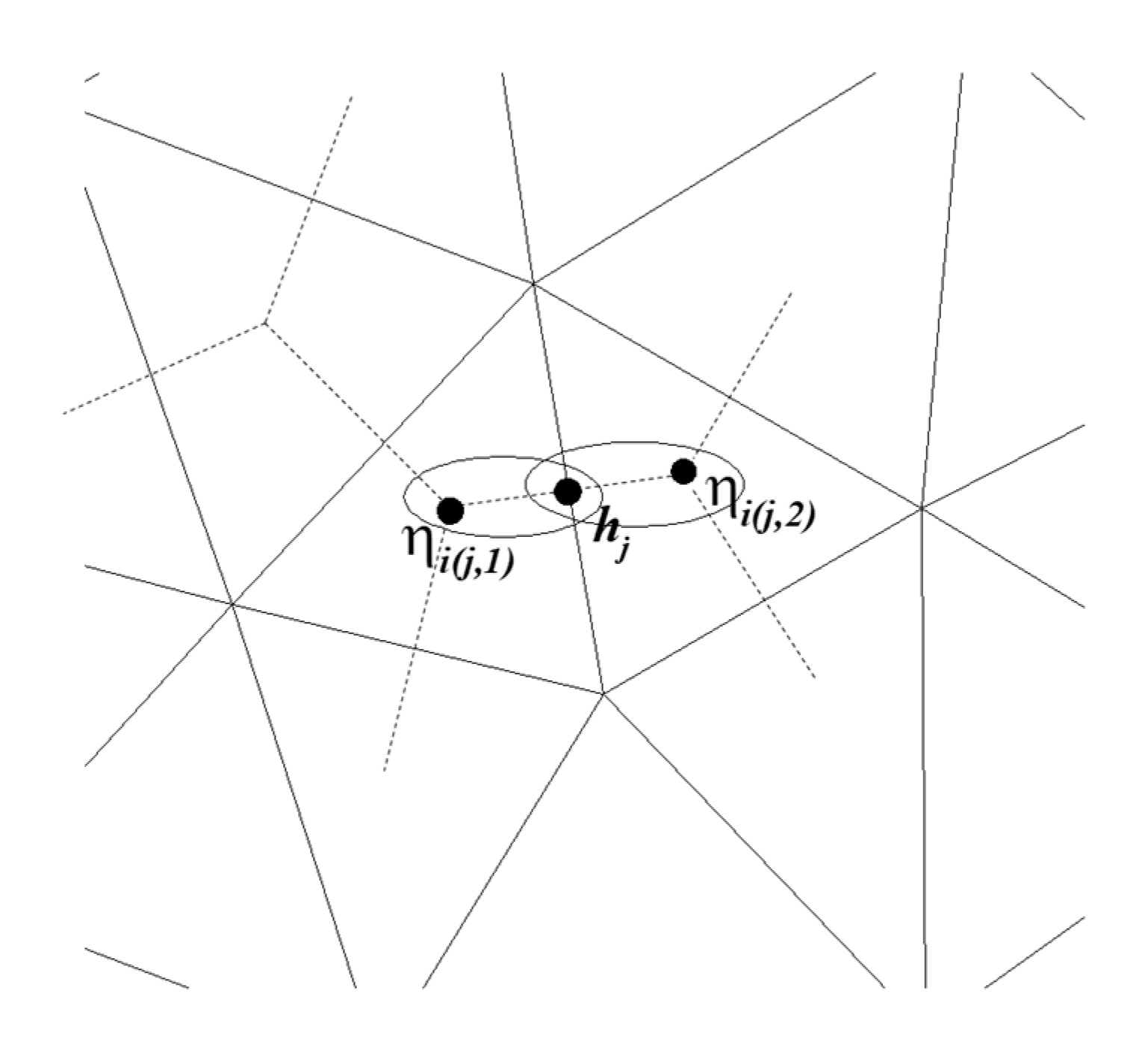
3. Unstructured Orthogonal Mesh and Index

We used an unstructured orthogonal mesh, both triangular and quadrilateral, in this model GOM. Once we construct the orthogonal meshes for the study site, the grid system has $N_p$ polygons (i.e., the total number of cells or elements), each having three (if it is triangular) or four sides (if it is quadrilateral), i.e., $S_i=3 \mathrm{or} 4$, where $i=1, 2, \dots , N_p$. The total number of sides in a grid system is defined as $N_s$, and the length of each side is defined as ${\lambda }_j$. Each side of the $i$th polygon is identified by $j\left(i,l\right), l=1, 2, \dots , S_i$, and the corresponding side lengths are defined as ${\lambda }_{j\left(i,l\right)}$. Finally, the distance between the centers of neighboring cells, which share the $j$th side, is denoted by ${\delta }_j$ (Figure 1); note that a definition of an orthogonal unstructured grid is well explained in several previous studies (e.g., [2,12]).

As shown in Figure 2, along the vertical direction, a finite difference discretization, which is not necessarily uniform, is adopted; the $k$th vertical layer has a height of $\mathsf{\Delta }{z}_k$, i.e., the distance between levels $k-1$ and $k$. The horizontal velocities and water surface elevation are defined at staggered locations as follows: The water surface elevation ${\eta }_i$, the density ${\rho }_i$, the salinity $S_i$, and the temperature $T_i$ are located at the center of the $i$th polygon; note that the salinity and temperature are not yet included in the current version, but we show this in Figure 2 for the clarity and to explain the baroclinic gradient term in the later section. The velocity component normal to each face of a prism is defined at the point of intersection between the face and the segment joining the centers of the two prisms that share the face (i.e., the face center).

4. Finite Volume and Difference Discretization

4.1. Momentum Equations in a New Coordinate

Equations (1) through (5) are invariant under solid rotation of the $x$- and $y$- axis on the horizontal plane. If we introduce a new coordinate system, $x^{*}$ and $y^{*}$, regarding the cell face, and by using the invariant property of the equations, the horizontal momentum Equations (1) and (2) can be expressed as follows

$$\frac{\partial u^{*}}{\partial t}+u^{*}\frac{\partial u^{*}}{\partial x}+v^{*}\frac{\partial u^{*}}{\partial y}+w\frac{\partial u^{*}}{\partial z}=-g\frac{\partial \eta }{\partial x}-\frac{g}{{\rho }_o}{{\displaystyle \int }}_{-h}^{\eta }\frac{\partial \rho }{\partial x}dz-\frac{1}{{\rho }_o}\frac{\partial P_a}{\partial x}+A_h\left(\frac{{\partial }^2{u}^{*}}{\partial x^2}+\frac{{\partial }^2{u}^{*}}{\partial y^2}\right)+\frac{\partial }{\partial z}\left(A_v\frac{\partial u^{*}}{\partial z}\right)+f{v}^{*}$$

(6)

$$\frac{\partial v^{*}}{\partial t}+u^{*}\frac{\partial v^{*}}{\partial x}+v^{*}\frac{\partial v^{*}}{\partial y}+w\frac{\partial v^{*}}{\partial z}=-g\frac{\partial \eta }{\partial y}-\frac{g}{{\rho }_o}{{\displaystyle \int }}_{-h}^{\eta }\frac{\partial \rho }{\partial y}dz-\frac{1}{{\rho }_o}\frac{\partial P_a}{\partial y}+A_h\left(\frac{{\partial }^2{v}^{*}}{\partial x^2}+\frac{{\partial }^2{v}^{*}}{\partial y^2}\right)+\frac{\partial }{\partial z}\left(A_v\frac{\partial v^{*}}{\partial z}\right)-f{u}^{*}$$

(7)

where $u^{*}$ and $v^{*}$ are the horizontal velocity components in a new coordinate system, $x^{*}$ and $y^{*}$; note that we omit asterisk $*$ at the $x^{*}$- and $y^{*}$- coordinates. The relations of velocity components between true horizontal velocities, $u$ and $v$, and coordinate transformed along each cell face, horizontal velocities, $u^{*}$ and $v^{*}$, are $u=u^{*}\cos \theta -v^{*}\sin \theta$, and $v=u^{*}\sin \theta +v^{*}\cos \theta$, where $\theta$ is the angle between the new $x$-axis, $x^{*}$, and the traditional $x$-axis, $x$, (Figure 3). For simplicity, * is omitted for the equations from here onwards.

Each term in Equation (6) can be discretized using different methods for the sake of accuracy and efficiency. When solving these equations, the two most significant bottlenecks arise from the barotropic gradient term and the vertical mixing term. Thus, we used the semi-implicit scheme for the barotropic gradient term and the implicit scheme for the vertical diffusion term. On the other hand, the advection, horizontal diffusion, Coriolis, and baroclinic terms are discretized by explicit methods; note that the semi-implicit scheme is also used in the air pressure term. More details in each term are explained in the following sections.

4.1.1. Barotropic Gradient and Vertical Mixing: (Semi-) Implicit Treatment

For the two implicit scheme applied terms, barotropic gradient and the vertical diffusion terms, the finite difference discretization for the velocity component normal to each vertical face of a prism with a staggered grid system can be derived from Equation (6) and takes the following forms:

The barotropic gradient term with a semi-implicit $\theta$ scheme:

$$u_{j,k}^{n+1}=u_{j,k}^n-g\frac{\Delta t}{{\delta }_j}\left[\theta \left({\eta }_{i\left(j,2\right)}^{n+1}-{\eta }_{i\left(j,1\right)}^{n+1}\right)+\left(1-\theta \right)\left({\eta }_{i\left(j,2\right)}^n-{\eta }_{i\left(j,1\right)}^n\right)\right]$$

(8)

The vertical diffusion term with the implicit scheme:

$$u_{j,k}^{n+1}=u_{j,k}^n+\frac{\Delta t}{\Delta z_{j,k}^n}\left[A_v{}_{j,k+1/2}\frac{u_{j,k+1}^{n+1}-u_{j,k}^{n+1}}{\Delta z_{j,k+1/2}^n}-A_v{}_{j,k-1/2}\frac{u_{j,k}^{n+1}-u_{j,k-1}^{n+1}}{\Delta z_{j,k-1/2}^n}\right]$$

(9)

Then, Equation (6) can be written as

$$\begin{gathered} u_{j,k}^{n+1}=u_{j,k}^n+F_{j,k}^n \\ -g\frac{\Delta t}{{\delta }_j}\left[\theta \left({\eta }_{i\left(j,2\right)}^{n+1}-{\eta }_{i\left(j,1\right)}^{n+1}\right)+\left(1-\theta \right)\left({\eta }_{i\left(j,2\right)}^n-{\eta }_{i\left(j,1\right)}^n\right)\right]+\frac{\Delta t}{\Delta z_{j,k}^n}\left[A_v{}_{j,k+1/2}\frac{u_{j,k+1}^{n+1}-u_{j,k}^{n+1}}{\Delta z_{j,k+1/2}^n}-A_v{}_{j,k-1/2}\frac{u_{j,k}^{n+1}-u_{j,k-1}^{n+1}}{\Delta z_{j,k-1/2}^n}\right] \end{gathered}$$

(10)

where $k=m_j, m_j+1, \dots , M_j^n$, thus $m_j$ and $M_j^n$ denote the lower and upper limit for the vertical $k$ index at $j$-th side and time step $n$. The $u_{j,k}^n$ is the horizontal velocity component normal to the $j$-th side of the $i$-th mesh (we omit the subscript $i$ in equations for convenience), at vertical level $k$ and time step $n$; $F$ is an explicit finite difference operator, which includes the remaining terms in Equation (6): nonlinear advection, baroclinic gradient, air pressure, horizontal diffusion, and Coriolis terms. Calculations of the term $F_{j,k}^n$ will be discussed in the following sections.

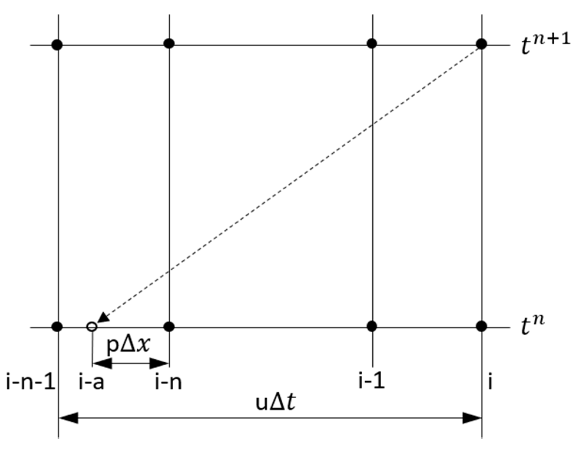
4.1.2. Nonlinear Advection: ELM

The Eulerian–Lagrangian Method (ELM) is used for solving the nonlinear advection terms in Equations (6) and (7) to take advantage of its simplicity, the enhanced stability, and accuracy. Most of the fundamental equations in fluid dynamics can be derived from principles in either Eulerian or Lagrangian forms. Consider the diffusion-free non-conservative advection equation in 1D

$$\frac{\partial c}{\partial t}+u\nabla c=0$$

(11)

where the $c\left(x,t\right)$ represents any scalar quantities or velocity vectors, $u$ is the velocity field, and $\nabla$ is a gradient operator. Then, the one-dimensional Eulerian advection Equation (11) can be expressed in the Lagrangian form as

$$\frac{Dc}{Dt}=0$$

(12)

The mathematical equivalence of Equations (11) and (12) follows from the definition of the total derivative,

$$\frac{D}{Dt}=\frac{\partial }{\partial t}+\frac{dx}{dt}\frac{\partial }{\partial x}$$

(13)

and the definition of the velocity,

$$\frac{d{x}_i}{dt}=u_i^{*}\left(x_1, x_2,x_3\right)$$

(14)

where $i=$ 1, 2, and 3, and * represents a linear interpolant between time step $n$ and $n+1$. When a Lagrangian numerical treatment is applied to Equation (12), the computational grid will be continuously deformed in the general case when $u$ is non-constant. For operational advantage, however, we will discretize Equation (12) on a fixed Eulerian grid system. Let us consider the one-dimensional time-dependent grid in the Eulerian grid shown in Figure 4. A finite difference scheme for Equation (11) is simply

$$c_i^{n+1}=c_{i-a}^n$$

(15)

where $c_{i-a}^n=c\left[\left(i-a\right)\Delta x,n\Delta t\right]$ and $n$ is time step, $i$ is any mesh or grid point, $t$ is the index at a grid point, and $a$ is the Courant-Friedrichs-Lewy (CFL) number. In general, the CFL number is not an integer, therefore, $\left(i-a\right)$ is not the index of a grid point, and a proper interpolation formula should be used to define $c_{i-a}^n$. The stability, numerical diffusion, and unphysical oscillations of Equation (15) depend on the interpolation formula chosen. If a linear interpolation between $\left(i-1\right)$ and $\left(i\right)$ is used to estimate $c_{i-a}^n$, one obtains the first-order upwind scheme. If a quadratic polynomial fit is used to interpolate between $\left(i-1\right)$, $(i$), and $\left(i+1\right)$, one obtains Leith’s [13] method. The ELM is well introduced by other researchers (e.g., [14,15,16]), thus, we do not re-introduce this method in detail here. The final form of the nonlinear term ($NL$) in the governing equation that we used in GOM is approximated as

$$NL=u_{j\left(i-a,l\right),k-b}^n$$

(16)

where $a$ and $b$ are the horizontal and vertical CFL numbers, respectively.

4.1.3. Coriolis: ELM

The Coriolis term in the equation is treated with the explicit ELM to take advantage of no time limitation for numerical stability. Consider the Coriolis term in Equation (6)

$$\frac{\partial u}{\partial t}=fv$$

(17)

By the explicit ELM, Equation (17) can be discretized as

$$u_{j,k}^{n+1}=u_{j,k}^n+\Delta tf{v}_{j,k}^{*}$$

(18)

where $v^{*}$ is the tangential velocity component in a right-hand coordinate system obtained by the Eulerian–Lagrangian method (see Figure 2). Finally, the Coriolis term ($COR)$ in Equation (6) is discretized by

$$COR=\Delta tf{v}_{j,k}^{*}$$

(19)

4.1.4. Horizontal Diffusion: The Finite Volume Cell-Centered Method

The conservation laws of fluid motion may be expressed mathematically in either differential or integral forms. When the integral form of the equation is utilized, the discretization of the equations is the finite volume method. To generalize the method, consider a two-dimensional heat conduction equation

$$\frac{\partial T}{\partial t}=A_h{\nabla }^{2}T$$

(20)

where ${\nabla }^2$ is the Laplace operator. Then, Equation (20) can be written as a conservative form

$$\frac{\partial T}{\partial t}=A_h\left[\frac{\partial }{\partial x}\left(\frac{\partial T}{\partial x}\right)+\frac{\partial }{\partial y}\left(\frac{\partial T}{\partial y}\right)\right]$$

(21)

Let $F=\left(\frac{\partial T}{\partial x}\right)$ and $G=\left(\frac{\partial T}{\partial y}\right)$, then Equation (21) is written as

$$\frac{\partial T}{\partial t}=A_h\left[\frac{\partial F}{\partial x}+\frac{\partial G}{\partial y}\right]$$

(22)

Equation (22) is integrated over an element’s area such as quadrilateral or triangular mesh, then

$${{\displaystyle \int }}_{P_i}^{}\left(\frac{\partial T}{\partial t}\right)dxdy=A_h{{\displaystyle \int }}_{P_i}^{}\left(\frac{\partial F}{\partial x}+\frac{\partial G}{\partial y}\right)dxdy$$

(23)

where $P_i$ denotes the $i$-th polygon. Subsequently, Green’s theorem is applied to the right-hand side of Equation (23). Recall that Green’s theorem converts area integrals to line integrals. Thus, Equation (23) is written as

$${{\displaystyle \int }}_{P_i}^{}\left(\frac{\partial T}{\partial t}\right)dxdy=A_h{{\displaystyle \oint }}_{P_i}^{}\left(Fdy-Gdx\right)$$

(24)

Finally, Equation (24) can be approximated as

$$T_i^{n+1}=T_i^n+A_h\frac{\Delta t}{A_i}{{\displaystyle \oint }}_{P_i}^{}\left(Fdy-Gdx\right)$$

(25)

Thus, the horizontal diffusion term (HD) in Equation (6) is approximated as:

$$HD=A_h\frac{\Delta t}{P_i}\left({{\displaystyle \oint }}_{P_i}^{}\left(Fdy-Gdx\right)\right)$$

(26)

4.1.5. Atmospheric Pressure: Semi-Implicit Method

The atmospheric pressure term in Equation (6) is approximated by the semi-implicit, method in time and forward difference in space. Consider the atmospheric pressure term in Equation (6)

$$\frac{\partial u}{\partial t}=-\frac{1}{{\rho }_o}\frac{\partial P_a}{\partial x}$$

(27)

The semi-implicit in time and forward differencing in spatial derivative produces the following finite difference equation of the form

$$\frac{u_{j,k}^{n+1}-u_{j,k}^n}{\Delta t}=-\frac{1}{{\rho }_o}\left(\frac{P_{a i\left(j,2\right)}^{n+\theta }-P_{a i\left(j,1\right)}^{n+\theta }}{{\delta }_j}\right)$$

(28)

and the atmospheric pressure term ($AP)$ in Equation (6) is approximated as

$$AP=-\frac{\Delta t}{{\rho }_o}\left(\frac{P_{a i\left(j,2\right)}^{n+\theta }-P_{a i\left(j,1\right)}^{n+\theta }}{{\delta }_j}\right)$$

(29)

The stability analysis indicates that this method is stable when $0.5\le \theta \le 1$. The values of $P_a^{n+\theta }$ are not calculated but provided explicitly as data at each time step.

4.1.6. Baroclinic Gradient: Explicit

The baroclinic gradient term (BG) in Equation (6) can be discretized with the explicit scheme

$$u_{j,k}^{n+1}=u_{j,k}^n-g\frac{\Delta t}{{\rho }_o{\delta }_j}\left[{\displaystyle \sum }_{kk=k}^M\Delta z_{j,kk}^n\left({\rho }_{i\left(j,2\right),kk}^n-{\rho }_{i\left(j,1\right),kk}^n\right)-\frac{\Delta z_{j,k}^n}{2}\left({\rho }_{i\left(j,2\right),k}^n-{\rho }_{i\left(j,1\right),k}^n\right)\right]$$

(30)

Then, the final numerical discretization of explicit term $F$ in Equation (10) is written as

$$F_{j,k}^n=NL+HD+COR+AP+BG$$

(31)

4.2. Boundary Treatment

4.2.1. Surface and Bottom Boundary Treatment for the Vertical Diffusion Term

While the vertical diffusion term in Equation (10) applies for a middle of a water column, new relations are required at both surface and bottom boundary layers to accelerate by the wind stress and to retard by the bottom friction. Using the shear stress, the vertical boundary conditions at the surface and the bottom yield the following formulae:

$$A_v{}_{j,M+1/2}\frac{u_{j,M+1}^{n+1}-u_{j,M}^{n+1}}{\Delta z_{j,M+1/2}^n}={\gamma }_T^{n+1}\left(u_{j,air}^{n+1}-u_{j,M}^{n+1}\right)$$

(32)

$$A_v{}_{j,m-1/2}\frac{u_{j,m}^{n+1}-u_{j,m-1}^{n+1}}{\Delta z_{j,m-1/2}^n}={\gamma }_B^{n+1}{u}_{j,m}^{n+1}$$

(33)

where $m$ and $M$ denote the bottom and top layers, respectively, and provide the surface and the bottom stress coefficients as ${\gamma }_T^{n+1}=\frac{A{v}_{j,M+1/2}^n}{\Delta z_{j,M+1/2}^n}$ and ${\gamma }_B^{n+1}=\frac{A{v}_{j,m-1/2}^n}{\Delta z_{j,m-1/2}^n}$, respectively. Then, the bottom stress coefficient ${\gamma }_B$ can be explained with the non-dimensional bottom drag coefficient, $C_{db}$. Then, we can approximate $C_{db}$ with Chezy’s formula and Manning’s roughness coefficient $n$, i.e., ${\gamma }_B=C_{db}\sqrt{\left(u^2+v^2\right)}=\frac{g}{C{z}^2}\sqrt{\left(u^2+v^2\right)}$, where $u$ and $v$ are velocities at the bottom layer, and $Cz$ is the Chezy friction coefficient, which can be formulated as

$$\mathrm{Cz}=\frac{R^{1/6}}{n}\approx \frac{H^{1/6}}{n}$$

(34)

where $R$ is the hydraulic radius, and $n$ is Manning’s roughness coefficient; in shallow estuaries, the hydraulic radius can be approximated by the total water depth.

Similarly, the boundary conditions at the free surface are specified by the prescribed wind stresses

$${\rho }_o{A}_v\frac{\partial u}{\partial z}={\tau }_{wx}={\rho }_a{C}_{da}{u}_w\sqrt{u_w^2+v_w^2}={\rho }_a{\gamma }_T{u}_w$$

(35)

$${\rho }_o{A}_v\frac{\partial v}{\partial z}={\tau }_{wy}={\rho }_a{C}_{da}{v}_w\sqrt{u_w^2+v_w^2}={\rho }_a{\gamma }_T{v}_w$$

(36)

where ${\tau }_{wx}$ and ${\tau }_{wy}$ are the wind stresses in $x$ and $y$ directions at the free surface; ${\rho }_o$ and ${\rho }_a$ are the density of the water and the air, respectively; $u_w$ and $v_w$ are the components of wind speed measured at some distance above the free surface; and $C_{da}$ is the surface drag coefficient. Then, the surface drag coefficient is now calculated by the empirical relationships such developed by either Garratt [17] or Smith [18], which are adopted in this model.

$$C_{da}=0.001\left(0.75+0.067W_s\right), \mathrm{Garratt} \left(1997\right)$$

(37)

$$C_{da}=0.001\left(0.61+0.063W_s\right), \mathrm{Smith} \left(1980\right)$$

(38)

where $W_s$ is the wind speed measured at 10 m above the water surface.

4.2.2. Treatment of Open Boundary Conditions

The tidal open boundary condition for the surface elevation is prescribed by

$$\eta \left(x,y,t\right)={\displaystyle \sum }_{n=1}^N{a}_{n}cos\left(\frac{2\pi }{T_n}t+{\varphi }_n\right)$$

(39)

where $a_n$, $T_n$, and ${\varphi }_n$ are the amplitude, period, and phase angle of each tidal constituent, respectively. When open boundary conditions are provided in terms of the surface elevation, the normal velocity component is assumed to be of a zero slope while the tangential velocity component may be either (1) zero, (2) zero slope, or (3) computed from the momentum equations. In this model, it is assumed that the velocity gradients are zero at the open boundary.

4.3. Free Surface Equation

To obtain complete local and global mass conservation and stability, the free surface Equation (5) is discretized by the finite volume method. Consider a uniform rectangular mesh in the Cartesian coordinate, as shown in Figure 5. To obtain a semi-implicit finite volume equation, integrate Equation (5) over an area of an element $P_i$, then

$${{\displaystyle \int }}_{P_i}^{}\left(\frac{\partial \eta }{\partial t}\right)\Delta x\Delta y=-{{\displaystyle \int }}_{P_i}^{}\left(\frac{\partial }{\partial x}\left[{{\displaystyle \int }}_{-h}^{\eta }udz\right]+\frac{\partial }{\partial y}\left[{{\displaystyle \int }}_{-h}^{\eta }vdz\right]\right)\mathsf{\Delta }x\mathsf{\Delta }y$$

(40)

Now, a semi-implicit finite volume discretization for Equation (40) gives

$$\begin{array}{l}\left(\frac{{\eta }_i^{n+1}-{\eta }_i^n}{\mathsf{\Delta }t}\right)\mathsf{\Delta }x\mathsf{\Delta }y=\\ -\theta \left[\left(\frac{{\sum }_{k=m}^M\mathsf{\Delta }{z}_{j\left(i,1\right),k}^n{u}_{j\left(i,1\right),k}^{n+1}-{\sum }_{k=m}^M\mathsf{\Delta }{z}_{j\left(i,3\right),k}^n{u}_{j\left(i,3\right),k}^{n+1}}{\mathsf{\Delta }x}\right)\mathsf{\Delta }x\mathsf{\Delta }y+\left(\frac{{\sum }_{k=m}^M\mathsf{\Delta }{z}_{j\left(i,2\right),k}^n{v}_{j\left(i,2\right),k}^{n+1}-{\sum }_{k=m}^M\mathsf{\Delta }{z}_{j\left(i,4\right),k}^n{v}_{j\left(i,4\right),k}^{n+1}}{\mathsf{\Delta }\mathrm{y}}\right)\mathsf{\Delta }x\mathsf{\Delta }y\right]\\ -\left(1-\theta \right)\left[\left(\frac{{\sum }_{k=m}^M\mathsf{\Delta }{z}_{j\left(i,1\right),k}^n{u}_{j\left(i,1\right),k}^n-{\sum }_{k=m}^M\mathsf{\Delta }{z}_{j\left(i,3\right),k}^n{u}_{j\left(i,3\right),k}^n}{\mathsf{\Delta }x}\right)\mathsf{\Delta }x\mathsf{\Delta }y+\left(\frac{{\sum }_{k=m}^M\mathsf{\Delta }{z}_{j\left(i,2\right),k}^n{v}_{j\left(i,2\right),k}^n-{\sum }_{k=m}^M\mathsf{\Delta }{z}_{j\left(i,4\right),k}^n{v}_{j\left(i,4\right),k}^n}{\mathsf{\Delta }\mathrm{y}}\right)\mathsf{\Delta }x\mathsf{\Delta }y\right]\end{array}$$

(41)

where $\mathsf{\Delta }x={\lambda }_{j\left(i,2\right)}={\lambda }_{j\left(i,4\right)}$ and $\mathsf{\Delta }\mathrm{y}={\lambda }_{j\left(i,1\right)}={\lambda }_{j\left(i,3\right)}$.

If Equation (41) is generalized for any shape of polygons in the unstructured grid system, a semi-implicit finite volume discretization for the free surface equation at the center of each polygon is taken to be [1]:

$$\begin{array}{l}{P}_i{\eta }_i^{n+1}=P_i{\eta }_i^n-\theta \mathsf{\Delta }t{\displaystyle \sum }_{l=1}^{S_i}\left[S_{i,l}{\lambda }_{j\left(i,l\right)}{\displaystyle \sum }_{k=m}^M\mathsf{\Delta }{z}_{j\left(i,l\right),k}^n{u}_{j\left(i,l\right),k}^{n+1}\right]\\ -\left(1-\theta \right)\mathsf{\Delta }t{\displaystyle \sum }_{l=1}^{S_i}\left[S_{i,l}{\lambda }_{j\left(i,l\right)}{\displaystyle \sum }_{k=m}^M\mathsf{\Delta }{z}_{j\left(i,l\right),k}^n{u}_{j\left(i,l\right),k}^n\right]\end{array}$$

(42)

where $P_i$ denotes the area of the $i$-th polygon, i.e., $P_i=\mathsf{\Delta }x\times \Delta y$ in Figure 5, and $S_{i,l}$ is a sign function of flows at each side, which is defined as [1]

$$S_{i,l}=\frac{i\left[j\left(i,l\right),2\right]-2i+i\left[j\left(i,l\right),1\right]}{i\left[j\left(i,l\right),2]-i\left[j\left(i,l\right),1\right]\right]}$$

(43)

5. Solution Algorithm

5.1. Solution of Governing Equations

Including wind stress at the surface layer and bottom stress at the bottom layer, and re-arranging the original x-momentum Equation (10), then we have the following tridiagonal matrix form for the $i$-th water column from the surface to the bottom layer at the $j$-th side

$$A_j^n{U}_j^{n+1}=G_j^n-\theta g\frac{\Delta t}{{\delta }_j}\left[{\eta }_{i\left(j,2\right)}^{n+1}-{\eta }_{i\left(j,1\right)}^{n+1}\right]\mathsf{\Delta }{Z}_j^n$$

(44)

where

$$\begin{gathered} A_j^n=\left[\begin{array}{ccc}(\mathsf{\Delta }t{\gamma }_T^{n+1}+\mathsf{\Delta }{z}_{j,M}^n+a_{j,M-\frac{1}{2}}^n)& -a_{j,M-\frac{1}{2}}^n& \\ -a_{j,M-\frac{1}{2}}^n& (a_{j,M-\frac{1}{2}}^n+\mathsf{\Delta }{z}_{j,M-1}^n+a_{j,M-\frac{3}{2}}^n)& -a_{j,M-\frac{3}{2}}^n\\ & ·& \\ & ·& \\ & ·& \\ & -a_{j,m+\frac{1}{2}}^n& (a_{j,m+\frac{1}{2}}^n+\mathsf{\Delta }{z}_{j,m}^n+\mathsf{\Delta }t{\gamma }_B^{n+1})\end{array}\right], \\ {U}_j^{n+1}=\left[\begin{array}{c}{u}_{j,M}^{n+1}\\ u_{j,M-1}^{n+1}\\ ⋮\\ u_{j,m}^{n+1}\end{array}\right],\hspace{1em}\hspace{1em}\hspace{1em}\mathsf{\Delta }{Z}_j^n=\left[\begin{array}{c}\mathsf{\Delta }{z}_{j,M}^n\\ \mathsf{\Delta }{z}_{j,M-1}^n\\ ⋮\\ \mathsf{\Delta }{z}_{j,m}^n\end{array}\right], \\ {G}_j^n=\left[\begin{array}{l}\Delta z_{j,M}^n\left\{F_{j,M}^n-g\frac{\Delta t}{{\delta }_j}\left(1-\theta \right)\left({\eta }_{i\left(j,2\right)}^n-{\eta }_{i\left(j,1\right)}^n\right)\right\}+\mathsf{\Delta }t{\gamma }_T^{n+1}{u}_{j,a}^{n+1}\\ \mathsf{\Delta }{z}_{j,M-1}^n\left\{F_{j,M-1}^n-g\frac{\mathsf{\Delta }t}{{\delta }_j}\left(1-\theta \right)\left({\eta }_{i\left(j,2\right)}^n-{\eta }_{i\left(j,1\right)}^n\right)\right\}\\ \mathsf{\Delta }{z}_{j,m}^n\left\{F_{j,m}^n-g\frac{\mathsf{\Delta }t}{{\delta }_j}\left(1-\theta \right)\left({\eta }_{i\left(j,2\right)}^n-{\eta }_{i\left(j,1\right)}^n\right)\right\}\end{array}\right] \end{gathered}$$

(45)

with $a_{j,k\pm 1/2}^n=\Delta t\frac{A_{v_{j,k\pm 1/2}}^n}{\Delta z_{j,k\pm 1/2}^n}$, ${\gamma }_B=C_{db}\sqrt{u_m^2+v_m^2}$, and ${\gamma }_T=C_{da}\frac{{\rho }_a}{{\rho }_o}\sqrt{u_w^2+v_w^2}$.

If we substitute $U_j^{n+1}$ from Equation (44) into Equation (42), which is the free surface wave equation, and rearrange the equation, then we have

$$\begin{array}{l}{P}_i{\eta }_i^{n+1}-g\mathsf{\Delta }{t}^2{\theta }^2{\displaystyle \sum }_{l=1}^{S_i}\frac{{\lambda }_{j\left(i,l\right)}}{{\delta }_{j\left(i,l\right)}}{\left[{\left(\mathsf{\Delta }Z\right)}^T{A}^{-1}\mathsf{\Delta }Z\right]}_{j\left(i,l\right)}^n\left({\eta }_{i\left[j\left(i,l\right),2\right]}^{n+1}-{\eta }_{i\left[j\left(i,l\right),1\right]}^{n+1}\right)\\ =P_i{\eta }_i^n-\left(1-\theta \right)\mathsf{\Delta }t{\displaystyle \sum }_{l=1}^{S_i}{S}_{i,l}{\lambda }_{j\left(i,l\right)}{\left[{\left(\mathsf{\Delta }Z\right)}^{T}U\right]}_{j\left(i,l\right)}^n-\theta \mathsf{\Delta }t{\displaystyle \sum }_{l=1}^{S_i}{S}_{i,l}{\lambda }_{j\left(i,l\right)}{\left[{\left(\mathsf{\Delta }Z\right)}^T{A}^{-1}\mathrm{G}\right]}_{j\left(i,l\right)}^n\end{array}$$

(46)

Equation (46) has a strongly diagonal dominant, a symmetric linear sparse matrix system of $N_p$ equations for ${\eta }_i^{n+1}$, thus, it can be efficiently solved by an iterative matrix solver, e.g., a preconditioned conjugate gradient method. Once the new water surface elevation at the center of each polygon is computed, substitute ${\eta }_i^{n+1}$ into the momentum Equation (44); then, horizontal velocities at the new time level at each face, $U_j^{n+1}$, will be obtained. Equation (44) has a tridiagonal system, and it can be solved efficiently by a direct tri-diagonal algorithm such as the Thomas algorithm. Finally, the vertical component of the velocity can be obtained from the integration of the incompressible continuity Equation (4).

$$\begin{gathered} w_{i,k+1/2}^{n+1}=w_{i,k-1/2}^{n+1}-\frac{1}{P_i}{\displaystyle \sum }_{l=1}^{s_i}{S}_{i,l}{\lambda }_{j\left(i,l\right)}\mathsf{\Delta }{z}_{j\left(i,l\right),k}^n{u}_{j\left(i,l\right),k}^{n+1} \\ k=m, m+1, \dots , M-1 \end{gathered}$$

(47)

5.2. Treatment of Flooding and Drying

Once the free surface elevation has been computed throughout the computational domain, before proceeding to the next time step, some of the vertical grid spacings $\mathsf{\Delta }{z}_{j,k}^{n+1}$ must be updated to account for the new surface location. As shown in Figure 6, at each time step, the new total water depth at the polygon’s sides, $H_j^{n+1}$, may be defined as

$$H_j^{n+1}=max\left[0 \left(or dry\_depth\right),h_j+{\eta }_{i\left(j,1\right)}^{n+1}, h_j+{\eta }_{i\left(j,2\right)}^{n+1}\right]$$

(48)

According to the new total water depth, the vertical grid spacing $\mathsf{\Delta }{z}_j^{n+1}$ should be updated. Thus, an occurrence of zero value for the total water depth $H_j^{n+1}$ implies that all the vertical faces separating prisms between the water column $i\left(j,1\right)$ and $i\left(j,2\right)$ are dry and may become wet at a later time when $H_j^{n+1}$ becomes positive [1]. When the total water depth is equal to zero, the friction factor at that point will be assumed to be infinity, and, accordingly, the corresponding velocity $u$ or $v$ across the side of the cell is forced to vanish. The occurrence of a zero value for the total water depth in one side of a cell implies zero velocity or zero mass flux until the total water depth becomes positive i.e., the boundary shorelines, which are varying with time, are defined by the condition of no mass flux. This guarantees mass conservation over the computational domain. An element is considered a dry cell only if the total water depths at all sides are zero.

To reduce computational noise or oscillation due to a very small wet element, a minimum critical dry depth is defined except using “0” in Equation (48). Therefore, elements are considered a wet element when the total water depth is greater than the critical depth and dry elements when the total water depth is less than or equal to the critical dry depth. The drying process can take place not only along the coast but also in interior regions such as shoals. For a shallow estuary, even under moderate wind stresses, some interior points over shoals can be dried completely, whereas the surrounding elements are still wet. Similarly, when the sea surface elevation is at a previously flooded location, this element returns to a dry cell. Then, an isolated dry element will not be turned into a wet cell until at least one of the neighboring elements also turns into a wet element.

6. Model Verification with Analytical Solutions

In previous sections, Section 2, Section 3, Section 4 and Section 5, we showed governing equations, grid systems, numerical schemes, and solution algorithms used in GOM. These processes may be similar or identical to other models, such listed by Fringer et al. [11]. However, conveying this information into a computer machine language is all different, and we used a standard FORTRAN 90 for this. Even though these processes are well-proven and robust approaches, any mistake in the final coding process leads to failure. To check the final success of this project, we compared a newly developed model, GOM, to well-known analytical solutions.

6.1. Wind Setup

The steady-state wind-induced setup due to constant wind stress in a rectangular basin can be written as

$$\eta \left(x\right)=\frac{{\tau }_w}{\rho gH}\left(x-\frac{L}{2}\right)$$

(49)

where $\eta$ is the setup of the water surface, ${\tau }_w$ is the applied wind stress, $H$ and $L$ are the depth and length of the basin, respectively, and the $x$ is the distance from the origin. The horizontal grid used in the wind setup test is 21 × 5 cells with a length of 21 km and a width of 5 km. The depth of the computational domain is a constant 5 m, and the horizontal grid spacing is 1 km in both directions. Constant wind stress of 0.1 N/m² (i.e., 1 dyne/cm² is applied in the positive $x$-direction, and a time step of 30 s is used in the simulation. Both 2-dimensional (with one vertical layer) and 3-dimensional (with 5 vertical layers) setups are used to verify the model. Both analytical and numerical results are calculated/extracted from 0.5, 10.5, and 20.5 km from the origin and compared, and both 2D and 3D simulation results reached a steady-state condition in one day and are the same as the analytical results (

Table 1. Comparisons between analytical and simulated wind setup, where $\eta$ is the setup of the water surface.

$\mathit{x} \left(\mathbf{km}\right)$	${\mathit{\eta }}_{\mathit{a}\mathit{n}\mathit{a}\mathit{l}\mathit{y}\mathit{t}\mathit{i}\mathit{c}\mathit{a}\mathit{l}}\left(\mathbf{cm}\right)$	${\mathit{\eta }}_{2\mathit{D} \mathit{m}\mathit{o}\mathit{d}\mathit{e}\mathit{l}}\left(\mathbf{cm}\right)$	${\mathit{\eta }}_{3\mathit{D} \mathit{m}\mathit{o}\mathit{d}\mathit{e}\mathit{l}}\left(\mathbf{cm}\right)$
0.5	−2.04	−2.04	−2.04
10.5	0	0	0
20.5	2.04	2.04	2.04

and Figure 7).

6.2. Tidal Propagation with Constant Depth

Tide is the most significant phenomenon in the ocean, and thus tidal simulation is one of the most important applications of a coastal and estuarine hydrodynamic model. Lynch and Gray [19] derived the analytical solutions for tidally forced estuaries of various geometries and depths. If we consider only tidal propagation term, i.e., the barotropic gradient term, in the original momentum Equation (1), and the continuity Equation (5), the one-dimensional shallow water equations in Cartesian coordinates are

$$\frac{\partial U}{\partial t}+gh\frac{\partial \eta }{\partial x}=0$$

(50)

$$\frac{\partial \eta }{\partial t}+\frac{\partial U}{\partial x}=0$$

(51)

where $U=uh$ is the depth-integrated velocity in $x$-direction. Assuming a closed boundary at $x=l$ and an open boundary at $x=0$, the boundary conditions and initial conditions associated with Equations (50) and (51) are

$$\begin{array}{l}\mathrm{Boundary} \mathrm{conditions}:\\ U\left(l,x\right)=0\\ \eta \left(0,t\right)={\eta }_0+a·\sin \left(\omega t\right)\\ \mathrm{Initial} \mathrm{conditions}:\eta \\ \left(x,0\right)={\eta }_0\\ U\left(x,0\right)=0\end{array}$$

(52)

where $a$ is a tidal amplitude, $\omega$ is an angular frequency of the given tide, and ${\eta }_0$ is the initial water surface elevation measured from the undisturbed surface. With these initial and boundary conditions, the analytical solutions of the one-dimensional shallow wave equations for water surface elevation and velocity are [20]

$$\eta \left(x,t\right)=\frac{a·\cos \left(k\left(l-x\right)\right)}{\cos \left(kl\right)}\sin \left(\omega t\right)+{\displaystyle \sum }_{n=0}^{\infty }\left[\frac{-2a\omega }{lc\left(k_n^2-k^2\right)}\sin \left(k_{n}x\right)\sin \left({\omega }_{n}t\right)\right]+{\eta }_0$$

(53)

$$U\left(x,t\right)=\frac{ac·sin\left(k\left(l-x\right)\right)}{\cos \left(kl\right)}\cos \left(\omega t\right)+{\displaystyle \sum }_{n=0}^{\infty }\left[\frac{-2a\omega }{l\left(k_n^2-k^2\right)}\cos \left(k_{n}x\right)\cos \left({\omega }_{n}t\right)\right]$$

(54)

where $k$ is the wavenumber ($=\frac{2\pi }{L}$, where $L$ is the wavelength), $k_n=\frac{\left(2n+1\right)\pi }{2L}$, $l$ is the basin’s length, $n$ is the number of nodes, $x$ is the interested location measured from the origin, and $t$ is the time.

To compare the numerical solution with a linear analytical solution, a rectangular basin with a constant water depth of 10 m is considered. The model domain is discretized with 929 mixed elements (quadrilateral elements at the left and triangular elements at the right, $\Delta x=\Delta y=~2 \mathrm{km}$) and one vertical layer, as shown in Figure 8; note that the only reason we constructed a mixed grid in this problem was to prove our model’s capability to handle both triangular and rectangular grids. Input tidal forcing along the open boundary was set with 0.5 m of amplitude and a period of 12.42 h. The simulation time step was set to 30 min, and the test simulations were run with $\theta =1$ and $\theta =0.5$, respectively. It is noted that when using the implicit numerical scheme, i.e., $\theta =1$, numerical diffusion is introduced. Thus, the numerical solution should correspond to the first mode of the analytical solution, which corresponds to the first terms of Equations (53) and (54). If a semi-implicit scheme, i.e., $\theta =0.5$, is used, the numerical solution should be compared to the complete Equations (53) and (54) which include the higher mode solution [20,21].

The model results were extracted from three locations and compared with analytical solutions: (1) near the mouth (Station 1, $x=9 \mathrm{km}$, $y=15 \mathrm{km}$), (2) the middle of the basin (Station 2, $x=~ 29.1 \mathrm{km}$, $y=~14.7 \mathrm{km}$), and (3) near the closed boundary (Station 3, $x=~50.7 \mathrm{km}$, $y=~14.7 \mathrm{km}$). Model results with $\theta =1$, which should be compared with the first term in the analytical solution, agree well with analytical solutions (Figure 9). When $\theta =0.5$ is used, which should be compared with the full equation, the model results had a little discrepancy with analytical solutions but mostly agreed well (Figure 10).

6.3. Tidal Propagation with Nonlinear Advection

If nonlinear advection terms are included in the two-dimensional shallow water equations, it is not feasible to obtain an analytical solution. However, if the equations are reduced to one-dimension, we can obtain the harmonic series solution. Including only nonlinear advection and propagation terms, the original momentum Equation (1) and the continuity Equation (5) can be reduced as

$$\frac{\partial U}{\partial t}+\frac{\partial uU}{\partial x}+gh\frac{\partial \eta }{\partial x}=0$$

(55)

$$\frac{\partial \eta }{\partial t}+\frac{\partial U}{\partial x}=0$$

(56)

The boundary conditions are

$$\begin{gathered} u\left(l,t\right)=0 \\ \eta \left(0,t\right)=a·\sin \left(\omega t\right) \end{gathered}$$

(57)

With the boundary conditions, the analytical solution of Equations (55) and (56) up to the first order can be written as [20]

$$\eta \left(x,t\right)=\frac{a \cos \left(k\left(l-x\right)\right)}{\cos \left(kl\right)}\sin \left(\omega t\right)+\frac{a^{2}k}{8h co{s}^2\left(kl\right)}\left[x\sin \left(2k\left(l-x\right)\right)+\frac{l}{\cos \left(4kl\right)}\sin (2k\left(l+x)\right)-\frac{l}{\cos \left(4kl\right)}\tan \left(2kl\right)\cos \left(2x\left(l-x\right)\right)\right]\cos \left(2\omega t\right)$$

(58)

$$u\left(x,t\right)=\frac{1}{h}\left[\frac{ac \sin \left(k\left(l-x\right)\right)}{\cos \left(kl\right)}\cos \left(\omega t\right)+\frac{a^{2}k}{8h co{s}^2\left(kl\right)}\left[x\cos \left(2k\left(l-x\right)\right)+\frac{l}{2k}\sin (2k\left(l-x)\right)-\frac{l}{\cos \left(4kl\right)}\cos \left(2k(l+x\right))+\frac{l}{\cos \left(4kl\right)}\tan \left(2kl\right)\sin \left(2k\left(l-x\right)\right)\right]\sin \left(2\omega t\right)\right]$$

(59)

To test nonlinear advection term in the developed model, numerical simulations were conducted with the identical basin and tidal forcing conditions used in the previous test. Because the analytical solutions present up to the first mode solution, the implicit numerical solution, $\theta =1$, should be compared to the analytical solution. Numerical results were extracted at the same three locations as in the previous test (Figure 8) and compared with analytical solutions. The results show that the numerical and analytical solutions are in good agreement (Figure 11).

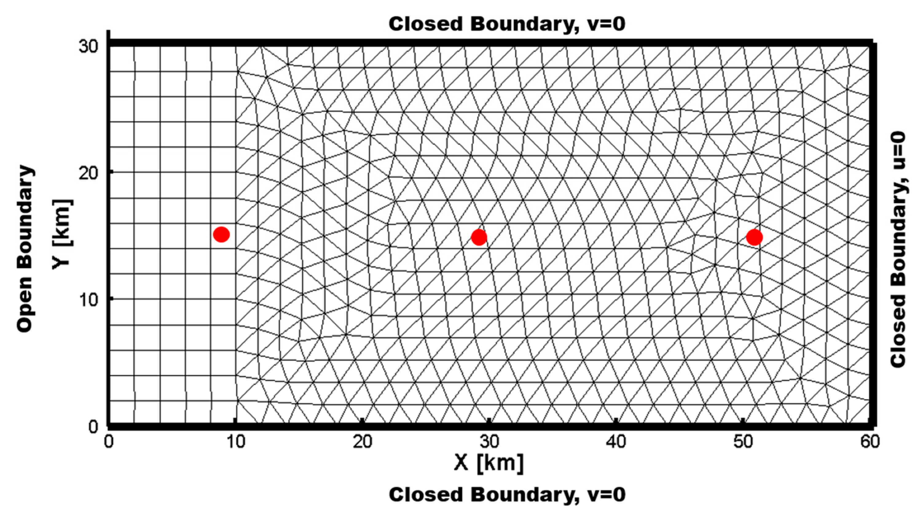
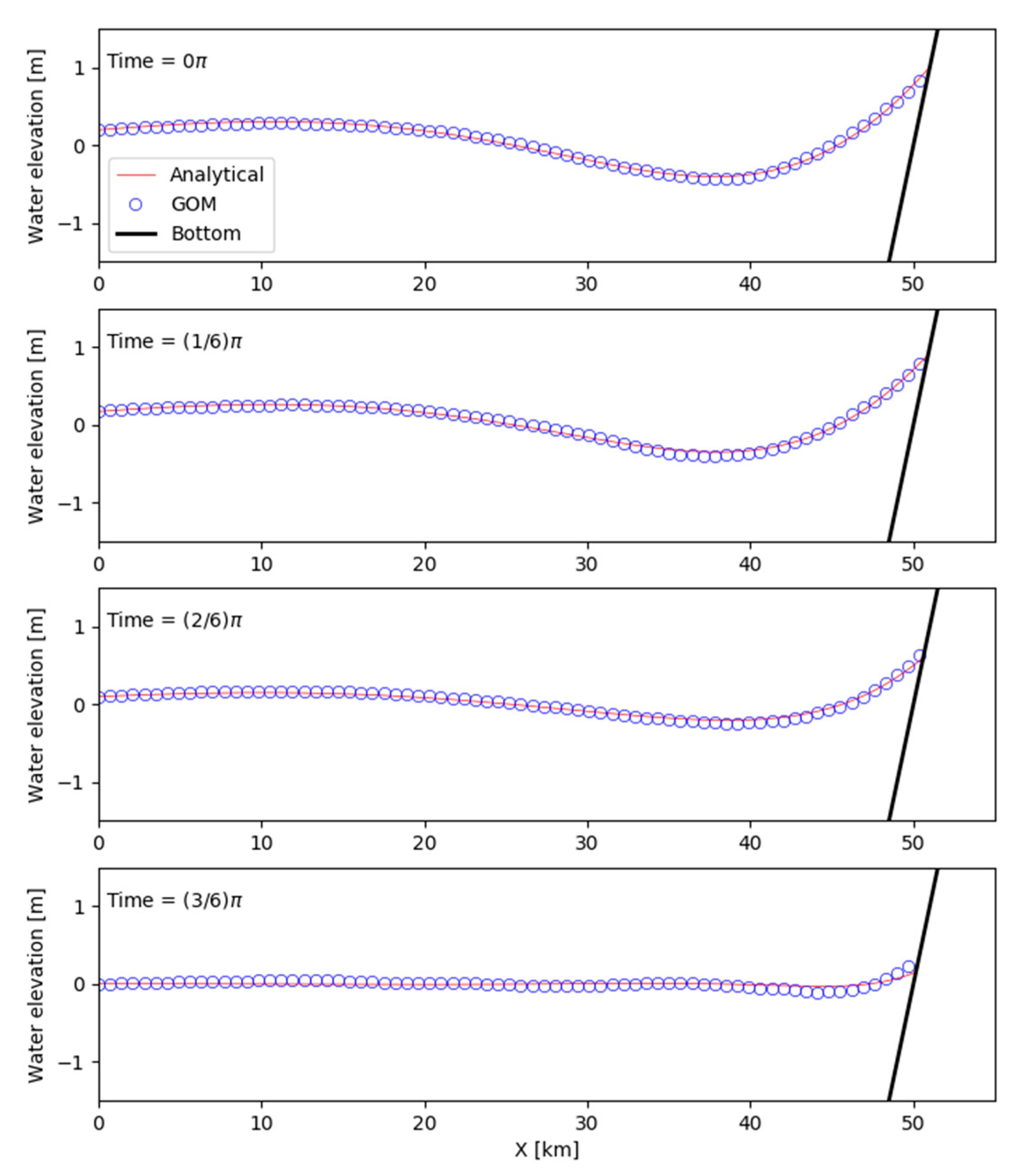
6.4. Quarter-Annular Harbor Test with a Sloping Bottom

Lynch and Gray [19] derived the analytical solutions for a tidally forced estuary with a flat bottom and a sloping bottom. The quarter-annular test, which contains spatially varying geometry and bathymetry, is one of the well-known test cases for testing the integrated numerical schemes of a developed ocean circulation numerical model. Numerical results will be poor with spurious oscillations or with excessive numerical dissipation if poor numerical schemes are used.

The analytical solutions for the Quarter-annular harbor test are well described by Lynch and Gray [19] and Lynch and Officer [22]. Neglecting nonlinear, Coriolis, and horizontal diffusion terms and assuming linear bottom friction, we can obtain the following vertically averaged equations

$$\frac{\partial u}{\partial t}+g\frac{\partial \eta }{\partial x}+\tau u=0$$

(60)

$$\frac{\partial v}{\partial t}+g\frac{\partial \eta }{\partial y}+\tau v=0$$

(61)

$$\frac{\partial \eta }{\partial t}+\frac{\partial hu}{\partial x}+\frac{\partial hv}{\partial y}=0$$

(62)

where $\eta$ is water surface elevation, $u$ and $v$ are vertically averaged velocities, $g$ is gravitational acceleration, and $\tau$ is the linear bottom friction coefficient. With the following boundary conditions: no flow boundaries at the closed end; $r=r_1$, which is the inner radius for the quarter-annular harbor at the open boundary; $r=r_0$, which is the outer radius for the quarter-annular harbor; and periodic tidal forcing $\eta ={\eta }_0 \cos \left(\omega t\right)$, where ${\eta }_0$ is amplitude, the analytic solutions for surface elevation and horizontal velocity are [19,22]

$$\eta \left(r,t\right)=Re\left\{\left(A{r}^{s_1}+B{r}^{s_2}\right)e^{i\omega t}\right\}$$

(63)

$$v\left(r,t\right)=Re\left\{\left(A{s}_1{r}^{s_1-1}+B{s}_2{r}^{s_2-1}\right)\frac{i\omega }{{\beta }^2{H}_0}{e}^{i\omega t}\right\}$$

(64)

where

$$\begin{array}{l}A=\frac{{\eta }_0{s}_2{r}_1^{s_2}}{s_2{r}_1^{s_2}{r}_2^{s_1}-s_1{r}_1^{s_1}{r}_2^{s_2}}, B=\frac{-{\eta }_0{s}_1{r}_1^{s_1}}{s_2{r}_1^{s_2}{r}_2^{s_1}-s_1{r}_1^{s_1}{r}_2^{s_2}}\\ s_1=-1+\sqrt{1-{\beta }^2}, s_2=-1-\sqrt{1-{\beta }^2}\\ {\beta }^2=\frac{\left({\omega }^2-i\omega \tau \right)}{g{h}_0}, h_0=\frac{h_1}{r_1^2}\\ \tau =\frac{N}{h^2}\left[\frac{{\lambda }^2\tanh \left(\lambda \right)}{\lambda +\left(\frac{{\lambda }^2}{K}-1\right)\tanh \left(\lambda \right)}\right]\\ K=\frac{kh}{N}, \lambda =\sqrt{\frac{i\omega h^2}{N}}\end{array}$$

(65)

and $N$ is the eddy viscosity; $k$ is the bottom friction.

The tested computational domain consists of a quarter of an annulus enclosed with land boundaries on three sides and an open ocean boundary on the outer edge. The inner radius has $r_1=60,960 m \left(=200,000 ft\right)$, and the outer radius has $r_0=152,400 m \left(=500,000 ft\right)$. The bathymetry along the inner radius $r_1$ is $h_1=3.048 m \left(=10 ft\right)$, and it drops quadratically at radius $r$ [23], i.e., $h_r=h_1{r}^2/r_1^2$. The discretization uses a radial spacing of $15,240 m \left(=50,000 ft\right)$ and an angular spacing of 11.25 degrees. Then, the computational domain consists of 48 rectangular cells with 63 nodes (Figure 12).

The model started from a state of rest, and periodic tidal force at the open boundary, advection, and quadratic bottom friction terms are activated. The elevation boundary is forced with a spatially uniform $M_2$ tide (tidal period = 12.42 h) with amplitude of 0.3048 m ($=1 ft)$. Total simulation time was set to 5 days with a time step of 174.656 s. Modeled water level time series are extracted every time step at three different locations in the domain, and the numerical results showed a good agreement with analytical solutions (Figure 13).

6.5. Wetting and Drying Test on Tidal Flats

Some shallow parts of coastal water bodies become wet and dry periodically in response to the tide, and, thus, the correct reproduction of the wetting and drying of the tidal flats is one of the desirable features of numerical tidal flow models based on shallow water equations. There are several different approaches to solve the wetting and drying process, and the major difference between all the models is the way to determine the drying and wetting cells and depths. The method to determine drying cells in the present model is based on Casulli and Walters [1], as explained in Equation (48).

To validate the wetting and drying scheme implemented in the developed model, we compared our model results with the analytical solution developed by Carrier and Greenspan [24]. The derivation of the analytical solution is well-reviewed in several papers (e.g., [20,25,26]). To compare with the analytical solution, a rectangular basin with a linearly sloping bottom is considered. The length and the width of the basin are set to 55 km and 100 m, respectively. The water depth at the origin, $x=0$ m, is set to 50 m, and the bottom slope,$\alpha$, is 1:1000; thus, the initial land and water interface is at $x=50$ km (Figure 14). The computational domain is divided by 550 $\times$ 1 quadrilateral elements ($\Delta x,\Delta y=100$ m). A periodic tide with an amplitude 0.2 m and a period of 1 h is applied at the open boundary, at $x=0$ m. Analytical results, which are originally given with non-dimensional variables, are converted to dimensional variables and compared with model results. Both analytical and numerical results are calculated and extracted every $\frac{1}{6}\pi$ tidal period and compared. Numerical simulation results show that the analytical and the numerical solutions are in good agreement, showing that the wetting and drying process implemented in GOM works well (Figure 15 and Figure 16).

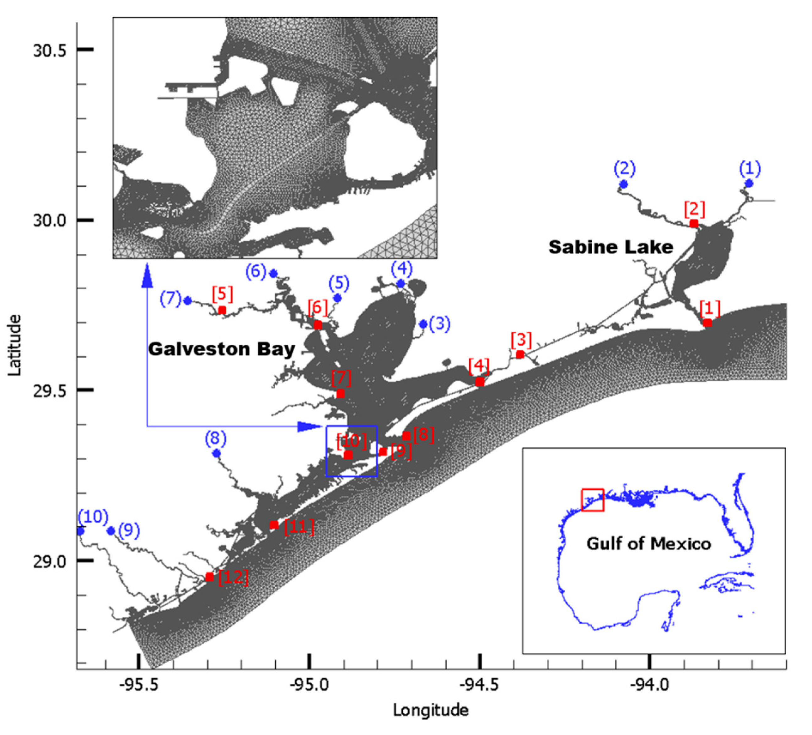
7. Model Application to the Texas Coast

Even though a model is verified with some analytical problems, it is sometimes not enough since each analytical problem is focused only on a specific term. For this reason, it is also important to verify the model with a realistic field problem, which includes all the physical aspects. The developed model, GOM, is applied to highly complex geometry, the northern Texas coast, to assess the performance of the developed model. Then, the model results are compared with the results of one of the well-known and widely used ocean circulation models, the Semi-Implicit Cross-Scale Hydroscience Integrated System Model (SCHISM). One of the main reasons why we chose the SCHISM here is its similarity in the horizontal grid system and its numerical scheme, the ELM, which is applied in the nonlinear advection term.

7.1. Model Domain and Grid Generation

We developed a model grid from the lower Galveston Bay to Sabine Lake (Figure 17). We used National Oceanic Atmospheric Administration (NOAA) ‘Medium Shoreline’ data for the land/sea boundary and ‘Coastal Bathymetry 2013’ from the Texas Natural Resources Information System (TNRIS) to correctly identify the locations of ship channels and the Intracoastal Waterway. The horizontal grid resolution varies from about 10 m at ship channels to about 3000 m at offshore boundaries. Most of the ship channels are resolved with quadrilateral elements, and otherwise, most of the model domains are covered by triangular elements. The offshore boundary for the model domain was set at about 15 km offshore from the coastline, and the final horizontal grids consist of 210,510 elements and 126,474 nodes.

After the horizontal grid was generated, the digital elevation models (DEMs) were interpolated onto the computational grid using the inverse distance weight (IDW) interpolation method. We used two different sources of DEMs: (1) the ETOPO1 Global Relief Model and (2) the Coastal Relief Model (CRM). The ETOPO1 is a 1 arc-minute global relief model of Earth’s surface that integrates land topography and ocean bathymetry, and it covers the entire Gulf of Mexico. The CRM has finer spatial resolution than ETOPO1; it provides one of the 3 arc-second, 1/3 arc-second, or 1/9 arc-second resolution DEMs depending on the area. Some portions of the study area are covered by either 1/3 or 1/9 arc-second DEMs, thus, both data are interpolated onto the grid; note that the minimum water depth was set to 1.0 m throughout the model domain.

7.2. Forcing Conditions and Model Setup

The developed model was validated for the one-month period in July 2017 and was forced by the tides, river discharge, and atmospheric wind stress. Three NOAA tide stations data, which are relatively close to the open boundary grids, were interpolated to the model boundary grids: Freeport (NOAA 8772447), Galveston Bay Entrance (NOAA 8771341), and Sabine Pass (NOAA 8770822) (Figure 17 and

Table 2. NOAA tide stations and United States Geological Survey (USGS) river gaging stations used in the model simulation.

# in Figure 17	NOAA Station ID	Station Name	USGS Station ID	Station Name
1	8770822	Sabine Pass	08030500	Sabine River
2	8770520	Rainbow Bridge	08041780	Neches River
3	8770808	High Island	08042558	Double Bayou
4	8770971	Rollover Pass	08067070	Trinity River
5	8770777	Manchester	08067500	Cedar Bayou
6	8770613	Morgan’s Point	08070200	San Jacinto River
7	8771013	Eagle Point	08074500	Buffalo Bayou
8	8771341	Galveston Bay Entrance	08078000	Chocolate Bayou
9	8771450	Galveston Pier 21	08116650	Brazos River
10	8771486	Galveston Railroad Br.	08117705	San Bernard River
11	8771972	San Luis Pass	-	-
12	8772447	Freeport	-	-

). Daily freshwater inflows obtained from the United States Geological Survey (USGS) gaging stations were specified at 10 river boundaries (Figure 17 and Table 2). These USGS stations are mostly located several kilometers upstream from the model river boundary nodes, but we assumed that there were no additional sources and sinks between the river gages and model river boundary nodes. For the wind stress, the North American Mesoscale forecast system (NAM) 6-hourly reanalysis data were interpolated onto the entire horizontal model grids. Spatially uniform bottom friction with Manning’s coefficient of 0.016 was used.

The still water condition was considered at the beginning, i.e., no water surface elevation disturbance and no water movement. The implicitness parameter was set to 0.6, and a two-dimensional simulation was considered. Finally, the model simulation time step was set to 600 s. Note that we also ran the SCHISM model with identical model setups to compare the simulation results.

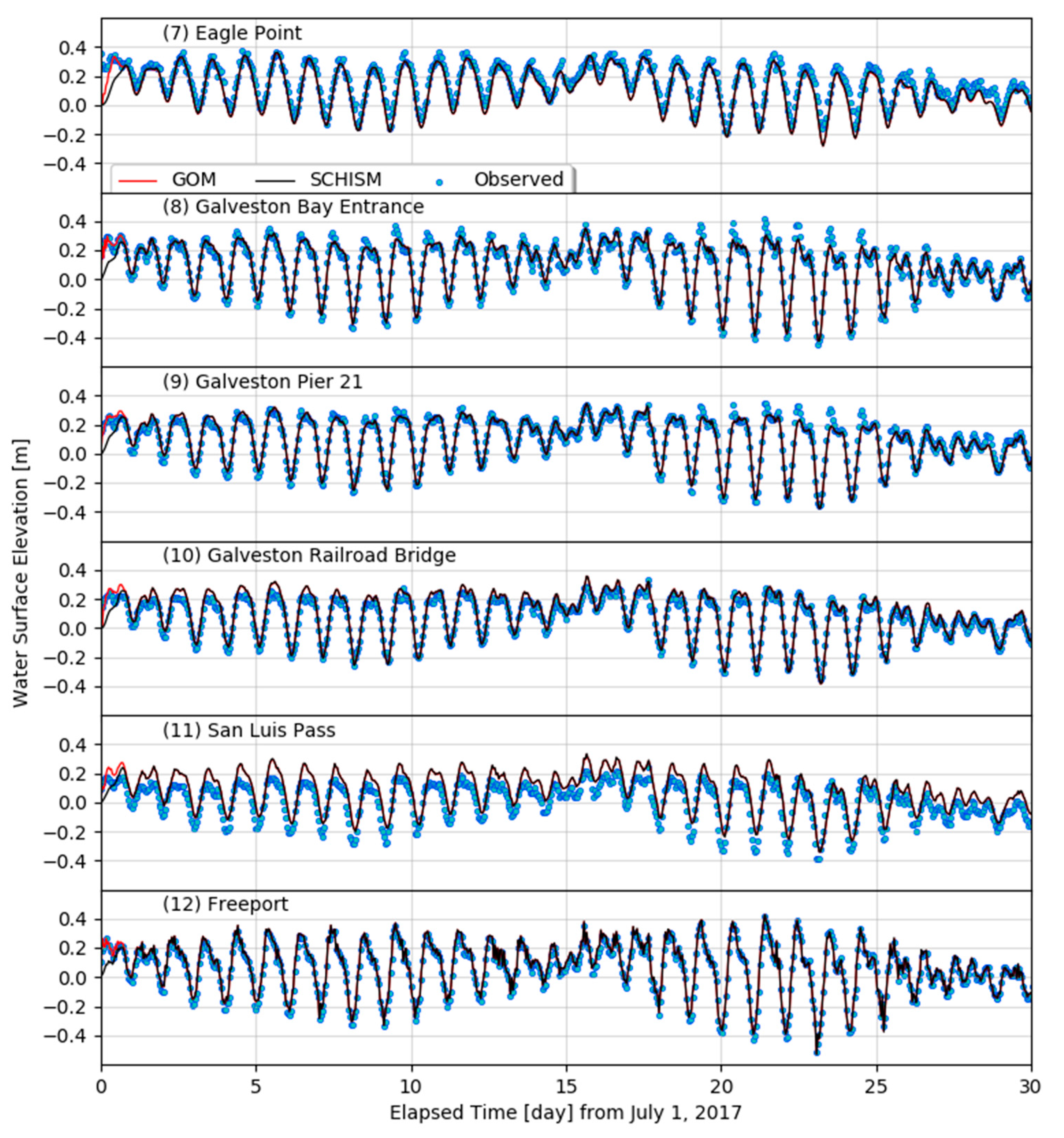
7.3. Model Validation

Model simulation results of the developed model, GOM, and the SCHISM were compared with the hourly measured water surface elevation data at twelve NOAA tide stations, which are shown in Figure 17 and Table 2. Figure 18 and Figure 19 show that the results of both models are almost identical and give a good agreement with observed water surface elevations. Note that there are some differences at the beginning of the simulation, but these were caused by applying a tide ramping up option only for the SCHISM simulation.

To better evaluate the model simulation results, we used two types of quantitative error analysis methods: mean absolute error (MAE) and predictive skill (it is also called skill or index of agreement), which was introduced by Willmott [27]. They are defined as follows [28,29]:

$$MAE=\frac{\sum \left|M_n-O_n\right|}{N}$$

(66)

$$Skill=1-\frac{\sum {\left(M_n-O_n\right)}^2}{\sum {\left(\left|M_n-\overline{O}\right|+\left|O_n-\overline{O}\right|\right)}^2}, \left(0\le Skill\le 1\right)$$

(67)

where $M_n$ and $O_n$ are $n$th modeled and observed data, respectively; $N$ is the total data number compared, and $\overline{O}$ is the mean observed value. The mean absolute error explains how much the modeled data deviate from the observed data, the value of skill explains how much the model can reproduce the observed data, and the value Skill = 1 indicates the perfect agreement [29].

When performing the error analysis, the first 5-day simulation results were excluded since the model required times to be stabilized. Overall, the developed model reproduces water surface elevations well throughout the entire model domain, and the results are quite similar to the SCHISM (

Table 3. Error analysis of the surface elevation simulation for both the SCHISM and GOM.

Tide Station	SCHISM		GOM		N
	MAE (cm)	Skill	MAE (cm)	Skill
(1) Sabine Pass	5.4	0.959	5.3	0.961	600
(2) Rainbow Bridge	5.5	0.945	5.5	0.945	600
(3) High Island	5.5	0.951	5.6	0.950	600
(4) Rollover Pass	6.4	0.934	6.5	0.931	600
(5) Manchester	10.8	0.897	10.5	0.901	600
(6) Morgan’s Point	9.1	0.909	8.8	0.912	600
(7) Eagle Point	5.0	0.957	5.1	0.955	600
(8) Galveston Bay Entrance	3.6	0.984	3.6	0.983	600
(9) Galveston Pier 21	3.2	0.981	3.3	0.980	600
(10) Galveston Railroad Br.	3.2	0.984	3.2	0.983	600
(11) San Luis Pass	8.1	0.890	8.1	0.887	600
(12) Freeport	2.2	0.994	2.1	0.995	600
Overall	5.7	0.951	5.6	0.951	7200

MAE: Mean Absolute Error. Skill: Predictive skill.

). The overall MAE is 5.6 cm for the GOM simulation, varying from 2.1 cm to 10.5 cm. The model skill value varies from 0.887 to 0.995, and the overall value is 0.951, indicating that the developed model performs well in a complex geometric study area with realistic forcing conditions. Note that there are some possibilities that we can improve the model simulation results by modulating bathymetry, bottom friction, and tidal boundary conditions. Applying spatially varying bottom friction is a common remedy to increase the model simulation results, and it is better to apply the correctness factors for the tidal amplitude and phase when the reference tide stations are off from the model’s boundary nodes. However, we ignored them since the goal of this simulation was not to improve the model simulation results but to validate the developed model’s performance.

8. Conclusions

We developed a three-dimensional numerical model with an orthogonal unstructured grid, either triangular or quadrilateral, for coastal and estuarine circulation, and we named it the General Ocean Model (GOM). This model is implemented with a combined finite difference and finite volume method. To eliminate the major simulation time step constraint which arises when solving shallow water equations, we used a semi-implicit method, which is stable when the implicitness factor, $\theta$, is between 0.5 and 1.0 for the wave propagation term. To moderate another time constraint, we adopted the Eulerian–Lagrangian method for the nonlinear advection term. In addition to the elimination of time constraints, exact numerical conservation is achieved by using the finite volume method.

We benchmarked an algorithm developed by Casulli and Walters [1], and this algorithm is simple, stable, and efficient. The algorithm is easy to expand from 2D to 3D equations, and by implementing ELM and semi-implicit schemes, this model can be used with fine spatial and vertical resolutions of the grid with relatively large time steps. We aimed to develop a model that can be used in coastal and estuarine regions, and, thus, the wetting and drying process is naturally achieved. In addition, this model can be used for a storm surge simulation since the atmospheric pressure term is included. The developed model, GOM, successfully passed five analytical tests we chose, and finally, it was verified with a realistic application to the Texas coast. The model simulation results were also compared with SCHISM to double-check the model performance.

There was another model that we initially considered to compare with our model, FVCOM by Chen et al. [5]. FVCOM is one of the leading and probably the most widely used finite volume ocean circulation models, thus, it might be worth comparing GOM with FVCOM, and they are as follows: First, FVCOM uses so-called “mode splitting”, while GOM solves 3D momentum equations directly from the integral forms, thus, no splitting error exists in GOM. Second, adopting the semi-implicit scheme in the recent FVCOM, users can have more freedom to apply this model with a highly refined unstructured model grid having a relatively large simulation time step. However, there is one difference in the horizontal mesh system when compared to our model—FVCOM only allows users to use a triangular mesh grid, while both triangular and quadrilateral grids can be used in our model, GOM. The study area, the Texas coast, is mostly shallow and fully connected with relatively narrow ship channels and the Gulf Intracoastal Waterway. This ship channel system can be better represented by quadrilateral grids than triangular grids to reduce the total grid size. Note that our model has not yet been parallelized, thus, the total number of the elements in the final grid is relatively important to reduce the total simulation time. Another advantage of using quadrilateral grids over triangular grids is their computational efficiency. We believe that adapting the advantages of both grids, i.e., grid refinement flexibility from triangular grids and efficiency from quadrilateral grids, gives users more accurate results and freedom to use this model. Another important difference in numerical schemes used in our model and FVCOM can be found in the treatment of the nonlinear advection term. Our model adopted the Eulerian–Lagrangian Method, while FVCOM uses the second-order explicit upwind method [5,30].

Even though this model is successfully tested, there are some aspects we want to improve when comparing it to well-recognized ocean circulation models, as mentioned by Fringer et al. [11]. With the Z-grid system (our model uses the current version of this), the model saved computational time in 3-dimensional simulations because the number of vertical grid cells is less in the shallow water area. However, the model requires one big surface layer, and this unwillingly reduces 3D to 2D in shallow water or an inundation area, thus, it is difficult to resolve 3D motions in the shallow area; this drawback will be improved by implementing the sigma ($\sigma$) grid. Another missing puzzle in this model, which aims to solve general coastal water motions, is the lack of transport equations. Even though this model includes the baroclinic gradient term, the salinity transport equation is not yet included. Implementation of these in this model will be our next task.

References

1. Casulli, V.; Walters, R.A. An unstructured grid, three-dimensional model based on the shallow water equations. Int. J. Numer. Methods Fluids 2000, 32, 331–348. [Google Scholar] [CrossRef]
2. Fringer, O.; Gerritsen, M.; Street, R. An unstructured-grid, finite-volume, nonhydrostatic, parallel coastal ocean simulator. Ocean Model. 2006, 14, 139–173. [Google Scholar] [CrossRef]
3. Zhang, Y.J.; Ateljevich, E.; Yu, H.-C.; Wu, C.H.; Yu, J.C.S. A new vertical coordinate system for a 3D unstructured-grid model. Ocean Model. 2015, 85, 16–31. [Google Scholar] [CrossRef]
4. Zhang, Y.J.; Ye, F.; Stanev, E.V.; Grashorn, S. Seamless cross-scale modeling with SCHISM. Ocean Model. 2016, 102, 64–81. [Google Scholar] [CrossRef] [Green Version]
5. Chen, C.; Liu, H.; Beardsley, R.C. An Unstructured Grid, Finite-Volume, Three-Dimensional, Primitive Equations Ocean Model: Application to Coastal Ocean and Estuaries. Journal of Atmospheric and Oceanic Technology 2003, 20, 159–186. [Google Scholar] [CrossRef]
6. Lai, Z.; Chen, C.; Cowles, G.W.; Beardsley, R.C. A nonhydrostatic version of FVCOM: 1. Validation experiments. J. Geophys. Res. Space Phys. 2010, 115, C11. [Google Scholar] [CrossRef] [Green Version]
7. Staniforth, A.; Côté, J. Semi-Lagrangian Integration Schemes for Atmospheric Models—A Review. Mon. Weather Rev. 1991, 119, 2206–2223. [Google Scholar] [CrossRef] [Green Version]
8. MacWilliams, M.; Gross, E. Hydrodynamic Simulation of Circulation and Residence Time in Clifton Court Forebay. San Franc. Estuary Watershed Sci. 2013, 11. [Google Scholar] [CrossRef] [Green Version]
9. MacWilliams, M.; Bever, A.J.; Gross, E.; Ketefian, G.; Kimmerer, W. Three-Dimensional Modeling of Hydrodynamics and Salinity in the San Francisco Estuary: An Evaluation of Model Accuracy, X2, and the Low-Salinity Zone. San Franc. Estuary Watershed Sci. 2015, 13. [Google Scholar] [CrossRef] [Green Version]
10. MacWilliams, M.L.; Ateljevich, E.S.; Monismith, S.G.; Enright, C. An Overview of Multi-Dimensional Models of the Sacramento–San Joaquin Delta. San Franc. Estuary Watershed Sci. 2016, 14. [Google Scholar] [CrossRef] [Green Version]
11. Fringer, O.B.; Dawson, C.; He, R.; Ralston, D.K.; Zhang, Y.J. The future of coastal and estuarine modeling: Findings from a workshop. Ocean Model. 2019, 143, 101458. [Google Scholar] [CrossRef]
12. Cheng, R.T.; Casulli, V. Evaluation of the UnTRIM Model for 3-D Tidal Circulation. Estuar. Coast. Model. 2001, 628–642. [Google Scholar] [CrossRef] [Green Version]
13. Leith, C.E. Atmospheric Predictability and Two-Dimensional Turbulence. J. Atmos. Sci. 1971, 28, 145–161. [Google Scholar] [CrossRef] [Green Version]
14. Cheng, R.T.; Casulli, V.; Milford, S.N. Eulerian-Lagrangian Solution of the Convection-Dispersion Equation in Natural Coordinates. Water Resour. Res. 1984, 20, 944–952. [Google Scholar] [CrossRef]
15. Oliveira, A.; Baptista, A.M. On the role of tracking on Eulerian-Lagrangian solutions of the transport equation. Adv. Water Resour. 1998, 21, 539–554. [Google Scholar] [CrossRef]
16. Lentine, M.; Grétarsson, J.T.; Fedkiw, R. An unconditionally stable fully conservative semi-Lagrangian method. J. Comput. Phys. 2011, 230, 2857–2879. [Google Scholar] [CrossRef] [Green Version]
17. Garratt, J.R. Review of Drag Coefficients over Oceans and Continents. Mon. Weather Rev. 1977, 105, 915–929. [Google Scholar] [CrossRef] [Green Version]
18. Smith, S.D. Wind Stress and Heat Flux over the Ocean in Gale Force Winds. J. Phys. Oceanogr. 1980, 10, 709–726. [Google Scholar] [CrossRef]
19. Lynch, D.R.; Gray, W.G. Analytic Solutions for Computer Flow Model Testing. J. Hydraul. Div. 1978, 104, 1409–1428. [Google Scholar]
20. Liu, Y. Two-Dimensional Finite-Difference Model for Moving Boundary Hydrodynamic Problems. Ph.D. Thesis, University of Florida, Gainesville, FL, USA, 1988. [Google Scholar]
21. Lee, J. Three-Dimensional Unstructured Finite Difference and Volume Model for Barotropic Coastal and Estuarine Circulation and Application to Hurricane Ivan (2004) and Dennis (2005). Ph.D. Thesis, University of Florida, Gainesville, FL, USA, 2008. [Google Scholar]
22. Lynch, D.R.; Officer, C.B. Analytic test cases for three-dimensional hydrodynamic models. Int. J. Numer. Methods Fluids 1985, 5, 529–543. [Google Scholar] [CrossRef]
23. Luettich, R.A.; Muccino, J.C.; Foreman, M.G.G. Considerations in the Calculation of Vertical Velocity in Three-Dimensional Circulation Models. J. Atmos. Ocean. Technol. 2002, 19, 2063–2076. [Google Scholar] [CrossRef] [Green Version]
24. Carrier, G.F.; Greenspan, H.P. Water waves of finite amplitude on a sloping beach. J. Fluid Mech. 1958, 4, 97–109. [Google Scholar] [CrossRef]
25. Sobey, R.J. Wetting and drying in coastal flows. Coast. Eng. 2009, 56, 565–576. [Google Scholar] [CrossRef] [Green Version]
26. Mungkasi, S.; Roberts, S.G. Approximations of the Carrier-Greenspan periodic solution to the shallow water wave equations for flows on a sloping beach. Int. J. Numer. Methods Fluids 2012, 69, 763–780. [Google Scholar] [CrossRef] [Green Version]
27. Willmott, C.J. Some Comments on the Evaluation of Model Performance. Bull. Am. Meteorol. Soc. 1982, 63, 1309–1313. [Google Scholar] [CrossRef] [Green Version]
28. Kim, C.-K.; Park, K. A modeling study of water and salt exchange for a micro-tidal, stratified northern Gulf of Mexico estuary. J. Mar. Syst. 2012, 96, 103–115. [Google Scholar] [CrossRef]
29. Lee, J.; Lee, J.; Yun, S.-L.; Oh, H.-C. Development of a finite volume two-dimensional model and its application in a bay with two inlets: Mobile Bay, Alabama. Cont. Shelf Res. 2017, 146, 13–27. [Google Scholar] [CrossRef]
30. Chen, C.; Huang, H.; Beardsley, R.C.; Liu, H.; Xu, Q.; Cowles, G. A finite volume numerical approach for coastal ocean circulation studies: Comparisons with finite difference models. J. Geophys. Res. Space Phys. 2007, 112, C03018. [Google Scholar] [CrossRef]
Figure 1. Orthogonal unstructured mesh and its notation used in the General Ocean Model (GOM), where P i is the i th polygon; λ j ( i , 1 ~ l ) is the length of the j th side when calling from the i th polygon; and δ j is the distance between the centers of neighboring cells that share the j th side.
Water 12 02752 g001
Figure 2. Location of computational variables, where η i , ρ i , S i , and T i denotes the water surface elevation, water density, salinity, and water temperature, respectively, which are defined at the center of the i th element; h j is the water depth which is defined at the j th side; u j , k * and v j , k * are the face normal and tangential velocities which are defined at the j th side; and k is the vertical layer index.
Water 12 02752 g002
Figure 3. Introduction of a new coordinate system, where x and y are the axes of the true east and north coordinate; x * and y * are the transformed axes assigned at each side; and θ is the angle between these two axes.
Water 12 02752 g003
Figure 4. The schematic diagram for the Eulerian grid on the Lagrangian frame, where i is the horizontal grid point; t is the time level; a is the CFL number; n and p are the integer part and the decimal part of a , respectively (i.e., a = n + p ,   0 p < 1 ) .
Water 12 02752 g004
Figure 5. Numerical stencils of a rectangular grid for the finite volume method, where λ j ( i , 1 )   ~   λ j ( i , 4 ) are the length of each cell face.
Water 12 02752 g005
Figure 6. Determination of wet and dry depth at an element face, where h j is the water depth at the j th side; η i ( i .1 ) is the water surface elevation at the i th element; and η i ( i .2 ) is the water surface elevation at the neighboring element which shares the j th side.
Water 12 02752 g006
Figure 7. Numerical results of the wind setup test (2D simulation results).
Water 12 02752 g007
Figure 8. Computation domain and mixed (triangular and quadrilateral) meshes for tidal propagation tests. Three red dots denote the model simulation comparison locations: from the left to the right—station 1, 2, 3.
Water 12 02752 g008
Figure 9. Comparison of water surface elevation for tidal propagation test at three locations with θ = 1.0 . Solid lines and circles represent analytical solutions and numerical results, respectively. ST_1, ST_2, and ST_3 denote result extraction locations shown in Figure 8.
Water 12 02752 g009
Figure 10. Comparison of water surface elevation for the tidal propagation test at three different locations with θ = 0.5 . Solid lines and circles represent analytical solutions and numerical results, respectively. ST_1, ST_2, and ST_3 denote result extraction locations shown in Figure 8.
Water 12 02752 g010
Figure 11. Comparison of water surface elevation for nonlinear advection at three different locations with θ = 1.0 . Solid lines and circles represent analytical solutions and numerical results, respectively. ST_1, ST_2, and ST_3 denote result extraction locations shown in Figure 8.
Water 12 02752 g011
Figure 12. Computational mesh for the quarter annular test. Upper panel: x–y plane, lower panel: x–z plane. Three data extraction locations are shown with numbers on the upper panel.
Water 12 02752 g012
Figure 13. Comparison of water surface elevation for the Quarter Annular test case at three different locations. Solid lines and circles represent analytical solutions and numerical results, respectively. ST_1, ST_2, and ST_3 denote result extraction locations shown in Figure 12.
Water 12 02752 g013
Figure 14. Definition sketch for Carrier and Greenspan [24] analytical solution on a linearly sloping beach, where MSL denotes the mean sea level; h is the water depth; η ( x , t ) is space and time-dependent water surface elevation; and α is the bottom slope.
Water 12 02752 g014
Figure 15. Comparison of wave profiles as predicted by theory (solid red lines) and numerical model (blue circles) of wetting and drying at time = 0 to π /2.
Water 12 02752 g015
Figure 16. Comparison of wave profiles as predicted by theory (solid red lines) and numerical model (blue circles) of wetting and drying at time = 2π/3 to π.
Water 12 02752 g016
Figure 17. The model domain and the horizontal grid. The ten blue dots denote included river boundaries, and the twelve red squares show National Oceanic Atmospheric Administration (NOAA) tide stations; the numbers are the corresponding station numbers in Table 2. The upper panel is the zoom-in of the selected coastal area at the lower Galveston Bay.
Water 12 02752 g017
Figure 18. Water surface elevation comparison between measurements (blue circles), GOM simulation results (solid red lines), and Semi-Implicit Cross-Scale Hydroscience Integrated System Model (SCHISM) simulation results (solid black lines) from tide stations 1 to 6.
Water 12 02752 g018
Figure 19. Water surface elevation comparison between measurements (blue circles), GOM simulation results (solid red lines), and SCHISM simulation results (solid black lines) from tide stations 7 to 12.
Water 12 02752 g019