1. Introduction
The vadose zone extends from the surface of the Earth down to the groundwater-table. This region is a habitat for bacteria and other microorganisms, some of which clean water while it travels through this zone. However, human activities in agriculture pollute the vadose zone and the groundwater with chlorine, nitrate [
1], and hormones [
2]. Industrial activities pollute the vadose zone and the groundwater with radioactive [
3], petrochemical [
4], and pharmaceutical [
5] compounds. Some of these acts of pollution have the potential to change the properties of the vadose zone and the aquifer irreversibly [
6] which in turn threatens the quality of groundwater in some regions permanently.
Land use can influence the amount of water in the vadose zone and the groundwater level [
7]. The extraction of groundwater for irrigation can lead to land subsidence, especially in arid regions [
8]. However, too much water in a slope may cause slope failure [
9].
All this underlines the importance of being able to simulate the vadose zone. Accurate simulations of the vadose zone can aid in the decision on how to react to an incident of pollution. Also, changes in land use and their impact on the recharge of the aquifer can be simulated. Furthermore, the decision to evacuate areas under a slope can be supported with accurate simulations of the vadose zone.
The Richards’-equation is widely used for modeling complex soil water dynamics in the vadose zone [
10]:
Here, represents the water content, for a 2-dimensional formulation and for a 3-dimensional consideration where is the vertical dimension, is the hydraulic conductivity, is the anisotropy tensor, is the pressure head, and is a sink term that models the in- and outflow over the system boundaries like evapotranspiration and precipitation. Thereby, Equation (1) formulates, that the change in water content is caused by the seepage flow that is caused by pressure and gravity and by the in- and outflow of water over the system boundaries.
The aim of this study is to show that the numerical simulation of Equation (1) can be sped up by using the free software library AMGCL [
11]. In
Section 2, an overview on how equation systems that arise from numerical discretizations of Equation (1) are solved is given. In
Section 3, AMGCL and PCSiWaPro [
12] are introduced. The metrics that are used to compare the performance of the solver in PCSiWaPro and AMGCL are introduced in
Section 4. In
Section 5, models are presented that are used to make the comparison of the solver in PCSiWaPro and AMGCL. The results obtained from the simulations of these models are presented in
Section 6.
Section 7 finishes this study with a discussion and conclusion.
2. Solving Equation Systems that Arise from the Numerical Discretization of the Richards’ Equation
There are several software packages available for the simulation of Equation (1). The most prominent are FEFLOW [
13], FEMWATER [
14], HydroGeoSphere [
15], HYDRUS [
16], PCSiWaPro, STOMP [
17], SWMS [
18], TOUGH3 [
19], VS2D [
20], and VSAFT2 [
21].
Equation (1) is usually simulated with the Finite Element Method [
22], the Finite Difference Method [
22] or the Finite Volume Method [
23].
Equation (1) is modelled with Finite Elements in FEFLOW, HydroGeoSphere, HYDRUS, PCSiWaPro, SWMS, and VSAFT2. The Finite Difference Method is used in STOMP, TOUGH3 and VS2D. The Finite Volume Method is considered in theoretical works [
24,
25], and also, there are some implementations of Equation (1) in the free numerical simulation toolbox OpenFOAM that discretize Equation (1) with the Finite Volume Method [
26,
27].
Whatever scheme is chosen to simulate Equation (1), the result is always an equation system of the form
where
is a matrix and
and
are vectors. In general, there are two ways to solve Equation (2) for
: The direct solution with the Gauss algorithm or “relatives” of it [
22], or iterative methods [
28].
The Gauss algorithm is computationally expensive which is why the Gauss algorithm is mainly used for small systems of equations. A “cousin” of the Gauss algorithm is the
LU-decomposition [
22], where one employs the Gauss algorithm to compute two matrices
and
where
is a lower triangular matrix and
is an upper triangular matrix, so that
. A “cousin” of
LU is the Cholesky factorization [
22], which demands
to be symmetric, where a lower triangular matrix
is computed so that
. The
LU-decomposition or the Cholesky-decomposition are popular in situations, where one wants to solve an equation system as in Equation (2) with constant matrix
and changing right hand sides
, because once the decompositions are computed,
can be solved, in case of the
LU-decomposition, as
, which in turn can be solved as
with
. Both of these equation systems are triangular, and therefore these systems of equations can be solved very fast.
In the case of iterative procedures, one computes a sequence of approximate solutions
, so that the residual
vanishes with growing
. There are several different schemes to compute this sequence. The most famous schemes are Gauss–Seidel [
28], Krylow Subspace [
28] algorithms, the Multigrid [
28] method, and Stone’s [
29] method.
The basic idea of Gauss–Seidel is to decompose the matrix where is a diagonal matrix, is a lower triangular matrix and is an upper triangular matrix. From this, a recursion can be built: . Instead of computing for a given vector or , one solves for which is computationally cheap since is a lower triangular matrix.
Krylow Subspace schemes employ the idea to compute the error
, and to create a subspace of dimension
from this error by defining
. Then, one chooses
so that
is perpendicular on
, where
is another subspace of dimension
. The simplest choice is
which is the starting point for the Conjugate Gradient algorithm [
28]. In the Conjugate Gradient algorithm, the update of approximation
to
is made by employing a search direction
, that is computed with the vectors
and
. The search directions
,
, … hold
for
, which explains the term “conjugate” in Conjugate Gradient. ORTHOMIN [
28] is a Krylow-type algorithm, where the search direction
is computed with the vectors
and
,
, …,
, where the memory
begins in the first iteration with
and grows with each iteration
until a maximum
is reached, where
is restarted with
. All Krylow Subspace algorithms aim at minimizing the norm of
, and the use of multiple past search directions as well as the reset of the number of past search directions every
iterations help ORTHOMIN to not get stuck in local minima. Another Krylow-type algorithm is BICGSTAB [
28] where the update of
is made with a search direction
and a vector
that is a scaled version of the resulting residual which in turn is caused by the update of
with
. Vector
is scaled, so that the update of
with
and
minimizes the norm of the residual
. This choice of
stabilizes the convergence of BICGSTAB. Aside from the Conjugate Gradient algorithm, ORTHOMIN and BICGSTAB, there are many other Krylow Subspace schemes. A good overview over these schemes can be found in [
28].
Krylow schemes can be sped up by preconditioning. In each iteration, the approximation error can be computed:
, then
. But since
is usually unknown and computationally expensive to compute, one searches for a matrix
so that
. A suitable matrix
is called a preconditioner. The most famous preconditioner is ILU (Incomplete
LU [
28]), where one attempts to approximate
by
, where
is a lower triangular matrix and
is an upper triangular matrix.
and
are not computed so that
because this would be too expensive computationally. A vector
is preconditioned with ILU by solving
for
, which is computationally cheap since
and
are both triangular matrices. However, this scheme cannot be parallelized, because in order to solve a triangular equation system, one has to solve the rows consecutively. Another popular preconditioner is SPAI (sparse approximate inverse [
30]). Here, one attempts to compute a matrix
, so that the sum over the squares of the entries of
is minimal, where
is the identity matrix. The advantage of SPAI is, that SPAI is constructed in a way that
can be computed massively parallel. There also exists polynomial preconditioning [
28]: consider
, where
is chosen, so that the largest absolute eigenvalue of
is smaller than 1, then the following relationship holds:
. This preconditioner is computationally very expensive since it demands many matrix-matrix-multiplications, but it can be massively parallelized. Also, this preconditioner demands enormous amounts of storage. Usually, the matrices involved with Finite Element, Finite Difference, or Finite Volume models are sparse, which means, that each row of the matrices has only a few entries which need to be kept in storage. If one multiplies matrices with each other, this sparsity is lost in general, which results in huge demands for storage.
Another approach to solve large equation systems is the Multigrid for which there are two variations: The geometric Multigrid and the algebraic Multigrid. In the case of the geometric Multigrid [
28], the discretization of the problem underlying Equation (2) is mapped to a sequence of consecutive coarser discretizations, and for each level of discretization, an equation system is created. Thereby, the equation system gets smaller with each level of discretization. On a given level, the current approximation error is reduced by a simple iterative scheme. This reduction of the approximation error is called relaxation. Simple algorithms are preferred for the relaxation, because one does not want to compute the exact solution, but rather a good approximation which can be computed fast. Algorithms like Gauss–Seidel or SPAI0 [
31] are popular algorithms for relaxation. SPAI0 defines a smoother
, where the matrix
is a diagonal matrix with
. Due to its simple structure,
can be computed in parallel. Also, the smoother SPAI0 can be highly parallelized, since it consists only of matrix-vector products and vector subtractions. On a given level, after the relaxation, the current approximation is either mapped to a coarser level or to a finer level. The mapping of the current approximation from a coarse- to a fine level is called prolongation, the mapping from a fine level to a coarse level is called restriction. There are different schemes like the V-cycle [
28], where one starts on the finest level, relaxes and restricts until the coarsest level is reached, and then relaxes and prolongs until the finest level is reached, where the sequence of restrictions and prolongations forms a “V”. In the W-cycle [
28], one arranges the restrictions and prolongations, so that they form a “W”. Since the dimensionality of the equation systems sinks with the coarseness of a level, the operations on the coarse levels are computationally very cheap. To sum up the idea of the geometric Multigrid, one maps a discretized geometry to a sequence of discretized geometries with increasing coarseness. For each of these grids, an equation system is formulated and the solution on each grid is approximated and mapped to the next grid. The problem with the geometric Multigrid is, however, that it shows difficulties with anisotropic coefficients of the underlying partial differential equation [
28]. These problems arise from the fact, that if the coefficients of the underlying partial differential equation are anisotropic, then errors are automatically introduced into the solution with the step from the fine grid to the coarse grid and vice versa. In the case of Equation (1), the coefficients are anisotropic, because each point in space has a pressure head which defines the hydraulic conductivity at that point. Therefore, if the pressure heads are anisotropic, then the hydraulic conductivity in Equation (1) is anisotropic. To illustrate the problem, consider the simple model of two nodes, where both nodes have a unique pressure head. If one would coarsen this simple model, one would restrict both nodes to one node. The node on the coarser level, however, can only reflect the hydraulic conductivity of at most one node from the finer level. Therefore, geometric Multigrid solvers perform poorly on discretizations of Equation (1).
In the case of the algebraic Multigrid, one does not bother with the geometry of the discretization, but rather one creates from the original equation system a sequence of equation systems with decreasing sizes [
28]. There are several schemes to compute the smaller equation system from a given equation system, the most famous schemes are the ones by Ruge and Stüben [
32] and Smoothed Aggregation [
33]. The basic idea of Ruge and Stüben is, to interpret a matrix
as a graph, where the entry
tells, how strongly the row
is connected to the row
. Then, one uses this strength of connection to decide, which rows need to be represented in the next coarser level, the
rows, and which rows need not to be represented, the
rows. In the Ruge and Stüben scheme,
is strongly negative coupled to
if
for some
. This strongly negative coupling is then used to define the set
. The transpose of this set is
. Therefore,
contains all
that are strongly negative coupled to
. Once, the sets
are computed for each row, one iteratively selects one
, puts this row into the
set, and the rows in
into the
set. Since this selection has to be performed iteratively, it cannot be parallelized. However, the information from the rows in the
set must not vanish, therefore the information from these rows is interpolated into the rows from the
set. Thereby, the problem with anisotropic coefficients in the geometric Multigrid is circumvented. In the Smoothed Aggregation algorithm, for each row
, the neighborhood is defined by
. For a given
,
is put into the
set, and the
in
are put into the
set. As with the Ruge and Stüben algorithm, the information from the rows in the
set is interpolated into the rows from the
set. In both algorithms, the solution is computed as with the geometric Multigrid once the equation systems are created.
The last approach to solve large equation systems that shall be considered in this paper is Stone’s Method. The core of Stone’s Method is to decompose A = S − T. Then, one can formulate the iterative scheme . Now, one has to solve this equation system for which is why one chooses , so that the decomposition S = LU, where is a lower triangular matrix and is an upper triangular matrix, is easy to compute.
FEFLOW offers direct Gaussian-type solvers, Krylow Subspace schemes and geometric and algebraic Multigrid. The Krylow schemes can be preconditioned with ILU. FEMWATER has Gauss–Seidel and preconditioned Conjugate Gradient solvers. The preconditioners are ILU and polynomial. HydroGeoSphere uses ORTHOMIN with ILU as preconditioner. HYDRUS, PCSiWaPro, STOMP and SWMS employ the Gauss-algorithm and preconditioned Conjugate Gradient with ILU as preconditioner. TOUGH3 offers the Gauss-algorithm and ILU-preconditioned Krylow Subspace schemes. VS2D uses Stone’s method as solver, and VSAFT2 has the ILU-preconditioned Conjugate Gradient as solver.
3. AMGCL and PCSiWaPro
As one can see, most software packages that solve the Richards’-equation with Krylow-type algorithms employ the ILU preconditioner. As shown above, ILU suffers from two aspects: On the one hand, ILU itself can in general only be a poor approximation to the real inverse, and on the other hand, ILU cannot be parallelized which makes preconditioning with ILU slow. Hence, there is a need for a highly parallelizable and yet accurate preconditioner for Krylow-type solvers of equation systems arising from discretizations of Equation (1). Because if one had a highly parallelizable and yet accurate preconditioner, then this preconditioner would speed up the solution of equation systems arising from discretizations of Equation (1). This speedup can then be translated into larger models that simulate the system in question in more detail, or one could use this additional time for simulating multiple scenarios.
Demidov published AMGCL, a C++-library with several Krylow-type solvers for which there are several algebraic Multigrid preconditioners available. AMGCL supports parallelization via OpenMP [
34], CUDA [
35] and MPI [
36]. In the standard settings, AMGCL performs preconditioning with an algebraic Multigrid and employs the V-cycle, and the equation system is coarsened until the coarsest level has at most 3000 nodes. On the coarsest level, a
LU-solver is employed. According to the standard settings of AMGCL, on each level two iterations of relaxation are performed. AMGCL offers algebraic Multigrid preconditioning according to the Ruge and Stüben scheme and Smoothed Aggregation. For the relaxation, there are Gauss–Seidel-, ILU- and SPAI-smoothers.
The development of PCSiWaPro began in the early 2000s when a group of scientists at the Technical University of Dresden took the numerical simulation code of SWMS_2D and extended this code by coupling the numerical kernel of SWMS_2D with a GUI that allows the user to create, modify and save 2-dimensional Finite Element models of the Richards′ equation. Also, PCSiWaPro extends SWMS_2D by offering a database that contains the properties of various soils according to DIN 4220 [
37] which is a standard for the designation, classification and deduction of soil parameters in Germany. The parameters of the soils can also be set manually. In order to extend the modelling capabilities of PCSiWaPro, the numerical kernel of SWMS_3D [
38] was added in 2019. Furthermore, the extension “Weather Generator” allows to create atmospheric boundary conditions from measurement data. PCSiWaPro uses the van Genuchten (which shall be abbreviated by VG) model [
39,
40] to describe the retention curve and the unsaturated hydraulic conductivity function of the soils in the model. As stated above, PCSiWaPro uses a Gaussian-type solver (for equation systems with less than 500 dimensions) and the ILU-preconditioned Conjugate Gradient (for equation systems with 500 or more dimensions) to solve equation systems that arise from the numerical approximation of Equation (1). A relative and an absolute tolerance of 1 × 10
−6 and a maximum of 1000 iterations are used as criteria for convergence and divergence. PCSiWaPro supports varying time step sizes. If the computation of a time step costs less than 4 calls of the solver, then the time step size is increased by a user defined factor. If the computation of a time step costs more than 6 calls of the solver, then the time step size is reduced by a user defined factor.
In order to investigate whether AMGCL can speed up the simulation of Equation (1), AMGCL was integrated into PCSiWaPro. The AMGCL solver was set up to employ BICGSTAB with an algebraic Multigrid-preconditioner which is based on Smoothed Aggregation where SPAI0 is used for relaxation.
BICGSTAB was chosen, due to its stabilized convergence behavior which makes the solver more robust. Initial tests revealed, that BICGSTAB preconditioned with algebraic Multigrid based on Smoothed Aggregation computes faster than BICGSTAB preconditioned with algebraic Multigrid based on the algorithm by Ruge and Stüben, therefore algebraic Multgrid with Smoothed Aggregation was chosen as preconditioner. SPAI0 was chosen for the relaxation, because SPAI0 was designed with the intention of massive parallelization, whereas, for example, the Gauss–Seidel scheme or ILU cannot be parallelized really well since triangular equation systems have to be solved.
Since the performance of AMGCL is to be compared with the ILU-preconditioned Conjugate Gradient solver, the absolute and relative tolerance of 1 × 10⁻⁶ and a maximum of 1000 iterations were coded into AMGCL to have a fair comparison.
PCSiWaPro with the AMGCL-solver with BICGSTAB as solver and algebraic Multigrid preconditioning based on the Smoothed Aggregation scheme with SPAI0 relaxation will be from now on referenced as PCSiWaPro AMGCL, whereas PCSiWaPro with the ILU-preconditioned Conjugate Gradient will be referenced as PCSiWaPro Original.
4. Method
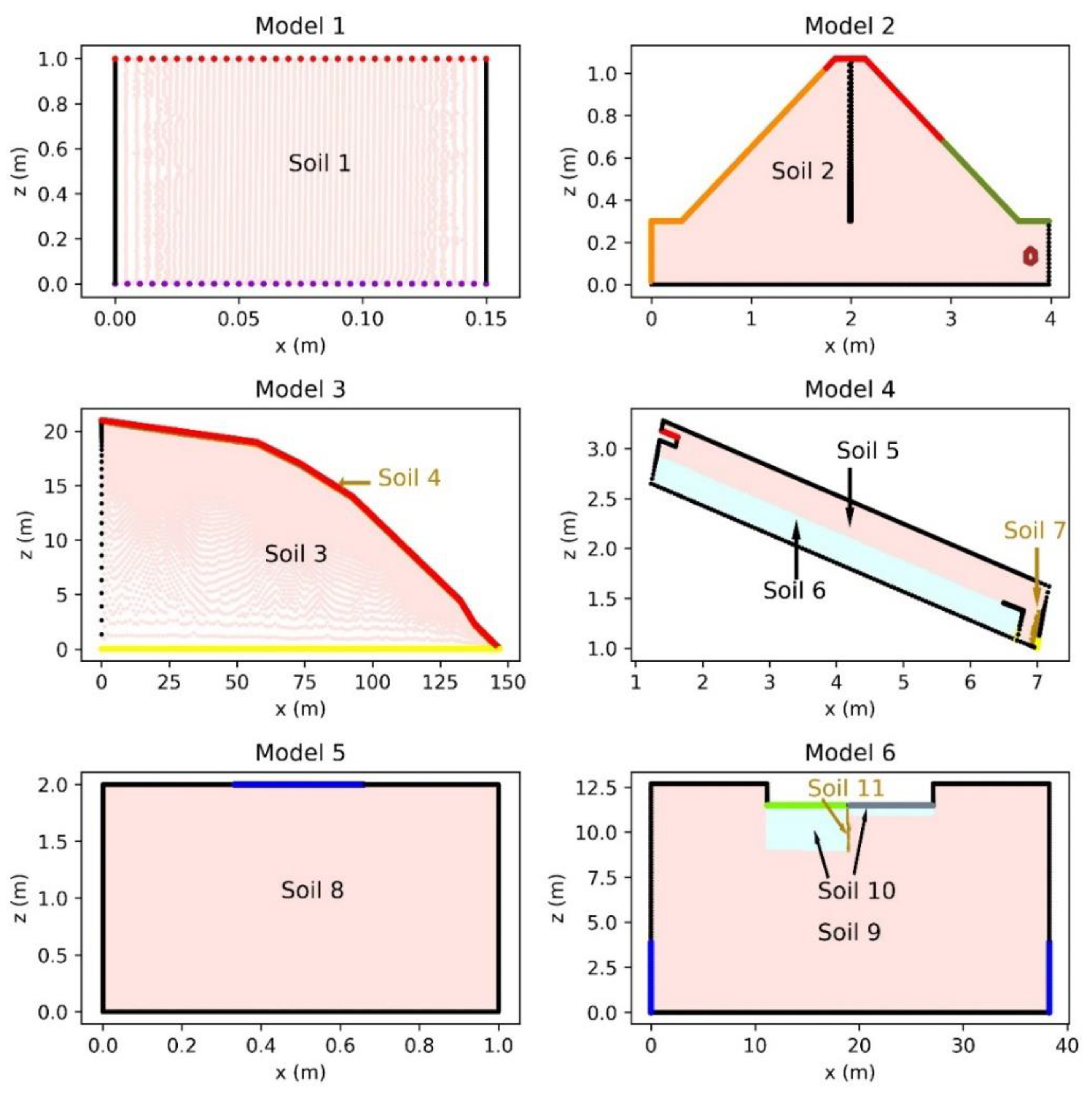
PCSiWaPro AMGCL and PCSiWaPro Original were compared on 7 synthetic models which will be described in the next section. These models were tuned with computations run in PCSiWaPro Original. The number of nodes in the models ranges from 7000 nodes to 2,400,000 nodes. Two models consider simple rectangular shapes, one model considers a rectangular cuboid, whereas the other four models consider more complex geometries. Four models consist of only one type of soil, the other three models each have at least two different kinds of soil.
All computations for the 6 2-dimensional models were run on a desktop PC running Windows 8 with an Intel Core i7-6700 CPU and 8 GB of RAM. During the computations, all 8 cores that are available on the i7-6700 CPU were used since PCSiWaPro and AMGCL both support parallelization with OpenMP. The 3-dimensional model was simulated on a computer running Windows Server 2012 r2 with an Intel Core i7-6800K CPU and 32 GB of RAM, and all 6 cores were used during the computations.
For the comparison of PCSiWaPro AMGCL with PCSiWaPro Original, three metrics were considered: the computational running time of the simulations which was measured in seconds, the R2-value between the pressure heads computed with PCSiWaPro Original and PCSiWaPro AMGCL, and the relative cumulative mass balance error (which shall abbreviated with RCMBE) computed with these two programs.
The
R2-value between the pressure heads computed with PCSiWaPro Original and PCSiWaPro AMGCL was chosen as a metric, because PCSiWaPro solves Equation (1) for the pressured heads.
The
R2-value was computed with Equation (3), where
is the vector of the pressure heads computed with PCSiWaPro Original at time point
, and
is the
-th entry of this vector.
is the mean of the values in
.
is the vector of the pressure heads computed with PCSiWaPro AMGCL at time point
, and
is the
-th entry of this vector. The nominator in Equation (3) is the squared error metric that computes the squared distance between the vectors
and
. This distance is normalized by the denominator. The normalization allows the
R2-value of different time steps or models to be compared. The best possible
R2-value is 1 when
and
are identical. The smaller the
R2-value, the greater the distance between the vectors
and
. The
R2-value was computed for every time step, and thereby, for each model, a time series of
R2-values was computed. The
R2-values were rounded to 4 digits after the decimal point.
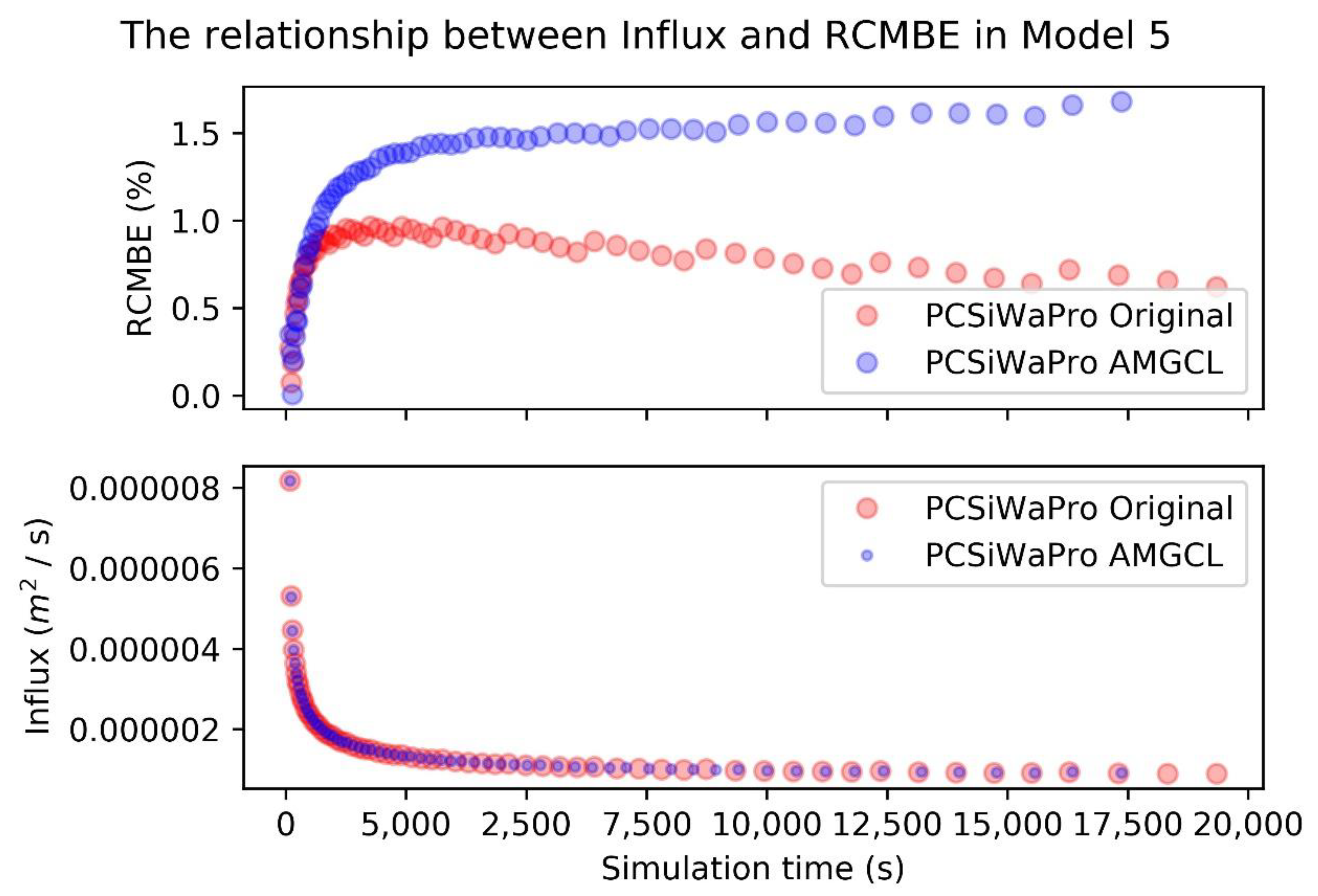
The RCMBE was computed with Equation (4). Here, is the amount of water in the model at time point . is the amount of water in the model at time point . is the root water uptake at time point . is the set of boundary nodes of the model. is the flow over the boundary in boundary node at time point . is the amount of water in element at time point , is the amount of water in element at time point . Therefore, the nominator in Equation (4) computes the absolute cumulative mass balance error at time point by considering the difference in water mass between the first time point and the current time point , the root water uptake between the first time point and the current time point , and the in- and outflow of water over the system boundaries between the first time point and the current time point . The denominator compares two terms and chooses the bigger one. The first term is the sum of the absolute changes in water mass in each element between the first time point and the current time point . The second term is the integral over the root water uptake and the sum of the absolute values of the mass transfer over system boundaries in the boundary nodes. The RCMBE is a proxy to how well the numerical approximation works, because if there were no numerical approximation and no rounding errors, the nominator in Equation (4) would be 0, because the change in water mass between the first and the current time point would be explained by the amount of water removed by the plants and the amount of water that left and entered the system over the boundaries. If the nominator in Equation (4) is not equal to 0, then the numerical approximation and rounding errors created or destroyed water artificially. The code of PCSiWaPro Original was used during the tuning of the models that will be presented in the next section. One aim of the tuning was, to keep the RCMBE below 1% for all time points in the simulation period.
7. Conclusions
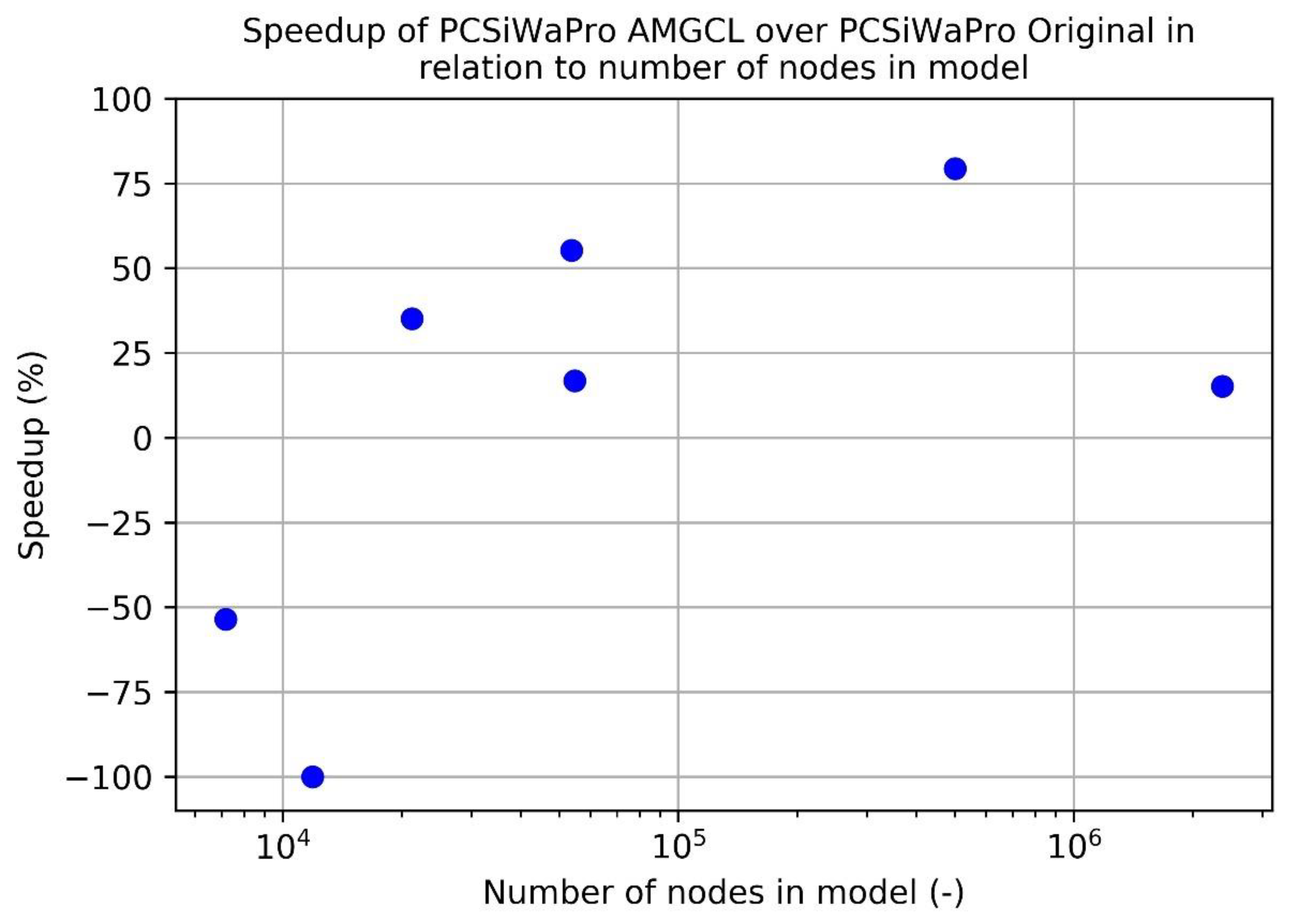
The comparisons above show, that PCSiWaPro AMGCL computes results that are of similar quality as the results computed with PCSiWaPro Original while being faster for larger models (20,000+ nodes). In all cases considered in this paper, the R2-values between the pressure heads computed with PCSiWaPro Original and PCSiWaPro AMGCL were in most models 1, and always greater than 0.999. Yet in one case, PCSiWaPro AMGCL computed results that violate against the rule to keep the RCMBE under 1%.
Also, for smaller models (<20,000 nodes), PCSiWaPro AMGCL computes slower than PCSiWaPro Original. Therefore, for larger models, PCSiWaPro Original may be replaced with PCSiWaPro AMGCL in order to speed up the computation.
The comparison of the number of calls of the solver showed, that the slower computational speed of PCSiWaPro AMGCL in comparison with PCSiWaPro Original in smaller models can only be explained by the numerical complexity of computing the algebraic Multigrid preconditioner. Therefore, for smaller models, the ILU-preconditioned Conjugate Gradient algorithm is a more efficient choice than BICGSTAB with algebraic Multigrid preconditioning.
This study only considered seepage flow that is modelled by Equation (1), but since BICCGSTAB can also deal with non-symmetric matrices [
28], BICGSTAB preconditioned with an algebraic Multigrid with Smoothed Aggregation and SPAI0 relaxation may be tested on transport problems in the vadose zone.
Another direction for future research is to evaluate whether further tuning of the models can increase the quality of the computational results computed with PCSiWaPro AMGCL while still being faster than PCSiWaPro Original.
Since PCSiWaPro uses the numerical discretization of the Richards’ equation that is also used in SWMS and HYDRUS, the findings of this study should also hold for SWMS and HYDRUS.
However, one finding of this study is the poor speedup caused by AMGCL with the 3-dimensional Model 7. The speedup of 15% is too little to be of practical relevance. Therefore, the performance of PCSiWaPro AMGCL has to be further evaluated for larger models. Unless more promising results are produced, we can only recommend to apply AMGCL in the simulation of small and medium scale problems (20,000 to 500,000 nodes).


