A Fuzzy Transformation of the Classic Stream Sediment Transport Formula of Yang


 ,
, 
Abstract
1. Introduction
2. Unit Stream Power Theory of Yang for Sediment Transport in Natural Rivers
3. “Fuzzy Twin”—The Physical Meaning
4. Materials and Methods
4.1. Experimental Data for the Derivation of Yang’s Formula
4.1.1. Nomicos’ Data (1956)
4.1.2. Vanoni and Brooks’ Data (1957)
4.1.3. Kennedy’s Data (1961)
4.1.4. Stein’s Data (1965)
4.1.5. Guy, Simons and Richardson’s Data (1966)
4.1.6. Williams’ Data (1967)
4.1.7. Schneider’s Data (1971)
4.2. Fuzzy Regression
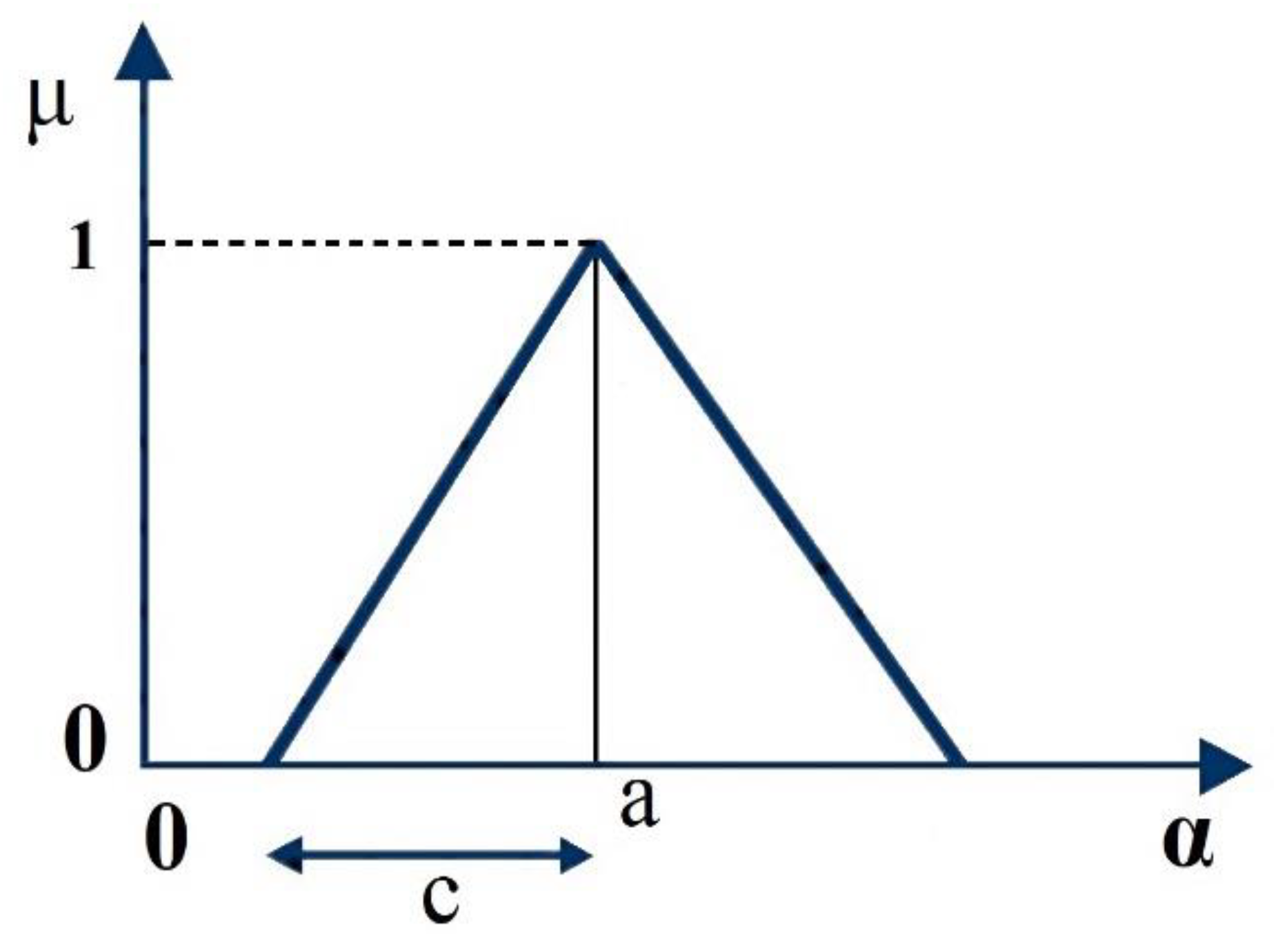
- The model is as follows:where is the fuzzy dependent variable; j = 1, …, m; i = 1, …, n; = (ai, ci) are symmetric fuzzy triangular numbers selected as coefficients; and x is the independent variable (Figure 1). In addition, n is the number of independent variables; m is the number of data; a is the central value (where μ = 1); and c is the semi-width.
- Determination of the degree h at which the data [(x1j, x2j, …, xnj), yj] is aimed to be included in the estimated number Yj:The constraints express the concept of inclusion in case that the output data are crisp numbers. In the examined case of the widely used model of Tanaka [47], a more soft definition of the fuzzy subsethood is used compared to the Zadeh [42] definition. Hence, the inclusion of a fuzzy set A into the fuzzy set B with the associated degree is defined as follows:In our case, since the data are crisp (for each individual data), the set A is only a crisp value (a point of data which must be included in the produced fuzzy band) and the fuzzy set B is a fuzzy triangular number. Hence, Equation (11) is equivalent to:It must be clarified that the above equations hold for a specified h-cut and not for every α-cut. Normally, the 0-strongcut is used since greater levels of h lead to a greater uncertainty.
- Determination of the minimization function (objective function) J. In the conventional fuzzy linear regression model, the objective function, J, is the sum of the produced fuzzy semi-widths for the data:where c0 is the semi-width of the constant term; and ci semi-width of the other fuzzy coefficients.Since fuzzy symmetric triangular numbers are selected as fuzzy coefficients, it can be proved that the objective function is the sum of the semi-widths of the produced fuzzy band regarding the available data:where the right and the left-hand side of the 0-strongcut, respectively.
- The problem results in the following linear programming problem:where ci ≥ 0, for i = 0, 1, …, n.In addition, many times, when data are classic numbers, we can easily approximate non-linear cases with the fuzzy linear regression model with the help of auxiliary variables. In this case, the total uncertainty (cumulative width) indicates incomplete complexity, whereas non-physical behavior is an indicator of overtraining [77], due to adoption of excessive complexity in non-linear models.
4.3. Implementation
5. Results
5.1. Determination of Yang’s Formula Independent Variables
5.2. Multiple Regression Analyses
5.2.1. Multiple Regression Analysis for the Reconstruction of the Unit Stream Power Formula
5.2.2. Fuzzy Regression Analysis
5.2.3. Validation
6. Conclusions
Author Contributions
Funding
Acknowledgments
Conflicts of Interest
Appendix A
References
- Gilbert, G.K.; Murphy, E.C. The Transportation of Debris by Running Water; US Geological Survey Professional Paper 86; US Government Printing Office: Washington, DC, USA, 1914.
- Rubey, W.W. Settling Velocities of Gravel, Sand and Silt Particles. Am. J. Sci. 1933, 148, 325–338. [Google Scholar] [CrossRef]
- Anderson, A.G.; Johnson, J.W. A Distinction Between Bed Load and Suspended Load in Natural Streams. Eos Trans. Am. Geophys. Union 1940, 21, 628–633. [Google Scholar]
- McCully, P. Silenced Rivers: The Ecology and Politics of Large Dams; Zed Books: London, UK, 1996. [Google Scholar]
- Kaffas, K.; Hrissanthou, V.; Sevastas, S. Modeling Hydromorphological Processes in a Mountainous Basin Using a Composite Mathematical Model and ArcSWAT. Catena 2018, 162, 108–129. [Google Scholar] [CrossRef]
- Kaffas, K. Development of Mathematical Model for Calculating Continuous Hydrographs and Sediment Graphs in a Basin Due to Rainfall. Ph.D. Thesis, Democritus University of Thrace, Xanthi, Greece, 28 June 2017. [Google Scholar]
- Graf, W.; Leitner, P.; Hanetseder, I.; Ittner, L.D.; Dossi, F.; Hauer, C. Ecological degradation of a meandering river by local channelization effects: A case study in an Austrian lowland river. Hydrobiologia 2016, 772, 145–160. [Google Scholar] [CrossRef]
- Spalevic, V.; Lakicevic, M.; Radanovic, D.; Billi, P.; Barovic, G.; Vujacic, D.; Sestras, P.; Darvishan, A.K. Ecological-Economic (Eco-Eco) Modelling in the River Basins of Mountainous Regions: Impact of Land Cover Changes on Sediment Yield in the Velicka Rijeka, Montenegro. Not. Bot. Horti Agrobot. Cluj-Napoca 2017, 45, 602–610. [Google Scholar] [CrossRef]
- Samaras, A.G.; Koutitas, C.G. Modeling the impact of climate change on sediment transport and morphology in coupled watershed–coast systems: A case study using an integrated approach. Int. J. Sed. Res. 2014, 29, 304–315. [Google Scholar] [CrossRef]
- Kondolf, G.M. PROFILE: Hungry water: Effects of dams and gravel mining on river channels. Environ. Manag. 1997, 21, 533–551. [Google Scholar] [CrossRef]
- Pisaturo, G.R.; Righetti, M. Sediment flushing from reservoir and ecological impacts. EPiC Ser. Eng. 2018, 3, 1692–1697. [Google Scholar]
- Yagci, O.; Celik, M.F.; Kitsikoudis, V.; Kirca, V.S.O.; Hodoglu, C.; Valyrakis, M.; Duran, Z.; Kaya, S. Scour patterns around isolated vegetation elements. Adv. Water Res. 2016, 97, 251–265. [Google Scholar] [CrossRef]
- Summerfield, M.A.; Hulton, N.J. Natural controls of fluvial denudation rates in major world drainage basins. J. Geophys. Res. 1994, 99, 13871–13883. [Google Scholar] [CrossRef]
- Galy, A.; France-Lanord, C. Higher erosion rates in the Himalaya: Geochemical constraints on riverine fluxes. Geology 2001, 29, 23–26. [Google Scholar] [CrossRef]
- Lavé, J.; Avouac, J.P. Fluvial incision and tectonic uplift across the Himalayas of central Nepal. J. Geophys. Res. 2001, 106, 26561–26591. [Google Scholar] [CrossRef]
- Turowski, J.M.; Rickenmann, D.; Dadson, S.J. The partitioning of the total sediment load of a river into suspended load and bedload: A review of empirical data. Sedimentology 2010, 57, 1126–1146. [Google Scholar] [CrossRef]
- Meyer–Peter, E.; Müller, R. Formulas for bed-load transport. In Proceedings of the International Association for Hydraulic Research, 2nd Meeting, Stockholm, Sweden, 7 June 1948. [Google Scholar]
- Camenen, B.; Larson, M.A. General formula for non-cohesive bed load sediment transport. Estuar. Coast. Shelf Sci. 2005, 63, 249–260. [Google Scholar] [CrossRef]
- Lane, E.W.; Kalinske, A.A. Engineering calculations of suspended sediment. Eos Trans. Am. Geophys. Union 1941, 22, 603–607. [Google Scholar] [CrossRef]
- van Rijn, L.C. Sediment transport, part II: Suspended load transport. J. Hydraul. Eng. 1984, 110, 1613–1641. [Google Scholar] [CrossRef]
- Ackers, P.; White, W.R. Sediment transport: New approach and analysis. ASCE J. Hydraul. Div. 1973, 99, 204–254. [Google Scholar]
- Yang, C.T. Incipient motion and sediment transport. ASCE J. Hydraul. Div. 1973, 99, 1679–1704. [Google Scholar]
- Schriften, D.V.W.K. Feststofftransport in Fließgewässern-Berechnungsverfahren für die Ingenieurpraxis; Heft 87; Verlag Paul Parey: Hamburg/Berlin, Germany, 1988. [Google Scholar]
- Einstein, H.A. The Bed-Load Function for Sediment Transportation in Open Channel Flows; No. 1488-2016-124615; US Department of Agriculture Technical Bulletin: Washington, DC, USA, 1950.
- Toffaleti, F.B. Definitive computation of sand discharge in rivers. ASCE J. Hydraul. Div. 1969, 95, 225–248. [Google Scholar]
- Karim, M.F.; Holly, F.M.; Kennedy, J.F. Bed Armoring Procedures in IALLUVIAL and Application to the Missouri River; No. 269; Iowa Institute of Hydraulic Research, University of Iowa: Iowa City, IA, USA, 1983. [Google Scholar]
- Yang, C.T. Unit stream power and sediment transport. ASCE J. Hydraul. Div. 1972, 98, 1805–1826. [Google Scholar]
- Engelund, F.; Hansen, E. A Monograph on Sediment Transport in Alluvial Streams; Teknisk Forlag: Copenhagen, Denmark, 1967. [Google Scholar]
- Zanke, U. Grundlagen der Sedimentbewegung; Springer: Berlin/Heidelberg, Germany, 1982. [Google Scholar]
- van Rijn, L.C. Closure to “Sediment transport, part I: Bed load transport”. ASCE J. Hydraul. Eng. 1984, 110, 1431–1456. [Google Scholar] [CrossRef]
- Yang, C.T. Sediment Transport: Theory and Practice, reprint ed.; Krieger: Malabar, FL, USA, 2003. [Google Scholar]
- Yang, C.T. Unit stream power equation for gravel. ASCE J. Hydraul. Eng. 1984, 110, 1783–1797. [Google Scholar] [CrossRef]
- Aqil, M.; Kita, I.; Yano, A.; Nishiyama, S. Analysis and prediction of flow from local source in a river basin using a neuro-fuzzy modeling tool. J. Env. Manag. 2007, 85, 215–223. [Google Scholar] [CrossRef] [PubMed]
- Zhu, S.; Heddam, S.; Nyarko, E.K.; Hadzima-Nyarko, M.; Piccolroaz, S.; Wu, S. Modeling daily water temperature for rivers: comparison between adaptive neuro-fuzzy inference systems and artificial neural networks models. Environ. Sci. Pollut. Res. 2019, 26, 402–420. [Google Scholar] [CrossRef] [PubMed]
- Tayfur, G.; Ozdemir, S.; Singh, V.P. Fuzzy logic algorithm for runoff-induced sediment transport from bare soil surfaces. Adv. Water Res. 2003, 26, 1249–1256. [Google Scholar] [CrossRef][Green Version]
- Chachi, J.; Taheri, S.M.; Pazhand, H.R. Suspended load estimation using L1—Fuzzy regression, L2—Fuzzy regression and MARS—fuzzy regression models. Hydrol. Sci. J. 2016, 61, 1489–1502. [Google Scholar] [CrossRef]
- Spiliotis, M.; Kitsikoudis, V.; Kirca, V.S.O.; Hrissanthou, V. Fuzzy threshold for the initiation of sediment motion. App. Soft Comp. 2018, 72, 312–320. [Google Scholar] [CrossRef]
- Zanke, U.C.E. On the influence of turbulence on the initiation of sediment motion. Int. J. Sed. Res. 2003, 18, 17–31. [Google Scholar]
- Spiliotis, M.; Kitsikoudis, V.; Hrissanthou, V. Assessment of bedload transport in gravel-bed rivers with a new fuzzy adaptive regression. Eur. Water 2017, 57, 237–244. [Google Scholar]
- Kitsikoudis, V.; Spiliotis, M.; Hrissanthou, V. Fuzzy regression analysis for sediment incipient motion under turbulent flow conditions. Environ. Proc. 2016, 3, 663–679. [Google Scholar] [CrossRef]
- Özger, M.; Kabataş, M.B. Sediment load prediction by combined fuzzy logic—Wavelet method. J. Hydroinf. 2015, 17, 930–942. [Google Scholar] [CrossRef]
- Kişi, Ö. Evolutionary fuzzy models for river suspended sediment concentration estimation. J. Hydrol. 2009, 372, 68–79. [Google Scholar] [CrossRef]
- Kişi, Ö.; Karahan, M.E.; Şen, Z. River suspended sediment modelling using a fuzzy logic approach. Hydrol. Proc. Int. J. 2006, 20, 4351–4362. [Google Scholar] [CrossRef]
- Lohani, A.K.; Goel, N.K.; Bhatia, K.S. Deriving stage—Discharge—Sediment concentration relationships using fuzzy logic. Hydrol. Sci. J. 2007, 52, 793–807. [Google Scholar] [CrossRef]
- Zadeh, L.A. Fuzzy sets. Inf. Control 1965, 8, 338–353. [Google Scholar] [CrossRef]
- Firat, M.; Güngör, M. Monthly total sediment forecasting using adaptive neuro-fuzzy inference system. Stoch. Environ. Res. Risk Assess. 2010, 24, 259–270. [Google Scholar] [CrossRef]
- Tanaka, H. Fuzzy data analysis by possibilistic linear models. Fuzzy Sets Syst. 1987, 24, 363–375. [Google Scholar] [CrossRef]
- Kaffas, K.; Hrissanthou, V. Estimate of continuous sediment graphs in a basin, using a composite mathematical model. Environ. Proc. 2015, 2, 361–378. [Google Scholar] [CrossRef]
- Kaffas, K.; Hrissanthou, V. Computation of hourly sediment discharges and annual sediment yields by means of two soil erosion models in a mountainous basin. Int. J. River Basin Manag. 2019, 17, 63–77. [Google Scholar] [CrossRef]
- Nakato, T. Tests of selected sediment—Transport formulas. J. Hydraul. Eng. 1990, 116, 362–379. [Google Scholar] [CrossRef]
- Baosheng, W.U.; van Maren, D.S.; Lingyun, L.I. Predictability of sediment transport in the Yellow River using selected transport formulas. Int. J. Sed. Res. 2008, 23, 283–298. [Google Scholar]
- Moore, I.D.; Burch, G.J. Sediment transport capacity of sheet and rill flow: Application of unit stream power theory. Water Res. Res. 1986, 22, 1350–1360. [Google Scholar] [CrossRef]
- Hui-Ming, S.; Yang, C.T. Estimating overland flow erosion capacity using unit stream power. Int. J. Sed. Res. 2009, 24, 46–62. [Google Scholar]
- Hrissanthou, V.; Hartmann, S. Measurements of critical shear stress in sewers. Water Res. 1998, 32, 2035–2040. [Google Scholar] [CrossRef]
- Yang, C.T. Unit stream power equations for total load. J. Hydrol. 1979, 40, 123–138. [Google Scholar] [CrossRef]
- Salas, J.D.; Shin, H.S. Uncertainty analysis of reservoir sedimentation. J. Hydraul. Eng. 1999, 125, 339–350. [Google Scholar] [CrossRef]
- Kleinhans, M.G. Flow discharge and sediment transport models for estimating a minimum timescale of hydrological activity and channel and delta formation on Mars. J. Geophys. Res. Planets 2005, 110. [Google Scholar] [CrossRef]
- Fischer, S.; Pietroń, J.; Bring, A.; Thorslund, J.; Jarsjö, J. Present to future sediment transport of the Brahmaputra River: Reducing uncertainty in predictions and management. Reg. Environ. Chang. 2017, 17, 515–526. [Google Scholar] [CrossRef]
- Beckers, F.; Noack, M.; Wieprecht, S. Uncertainty analysis of a 2D sediment transport model: An example of the Lower River Salzach. J. Soils Sediments 2017, 18, 3133–3144. [Google Scholar] [CrossRef]
- Azamathulla, H.M.; Ghani, A.A.; Fei, S.Y. ANFIS-based approach for predicting sediment transport in clean sewer. Appl. Soft Comp. 2012, 12, 1227–1230. [Google Scholar] [CrossRef]
- Nomicos, G.N. Effects of Sediment Load on the Velocity Field and Friction Factor of Turbulent Flow in an Open Channel. Ph.D. Thesis, California Institute of Technology, Pasadena, CA, USA, 1956. [Google Scholar]
- Vanoni, V.A.; Brooks, N.H. Laboratory Studies of the Roughness and Suspended Load of Alluvial Streams; Report No. E-68; Sedimentation Laboratory, California Institute of Technology: Pasadena, CA, USA, 1957. [Google Scholar]
- Kennedy, J.F. Stationary Waves and Antidunes in Alluvial Channels; Report No. KH-R-2; W.M. Keck Laboratory of Hydraulics and Water Resources, California Institute of Technology: Pasadena, CA, USA, 1961. [Google Scholar]
- Stein, R.A. Laboratory studies of total load and apparent bed-load. J. Geophys. Res. 1965, 70, 1831–1842. [Google Scholar] [CrossRef]
- Guy, H.P.; Simons, D.B.; Richardson, E.V. Summary of Alluvial Channel Data from Flume Experiment, 1956–1961; US Geological Survey Professional Paper: Washington, DC, USA, 1966.
- Williams, G.P. Flume Experiments on the Transport of a Coarse Sand; US Geological Survey Professional Paper: Reston, VA, USA, 1967.
- Schneider, V.R. Personal Communication of Yang. Data Collected from an 8-Foot Wide Flume at Colorado State University; Colorado State University: Fort Collins, CO, USA, 1971. [Google Scholar]
- Simons, D.B.; Richardson, E.V.; Albertson, M.L. Flume studies using medium sand (0.45 mm); US Geological Survey Water-Supply Paper: Washington, DC, USA, 1961.
- Inter-Agency Committee on Water Resources, Subcommittee on Sedimentation. Some Fundamentals of Particle Size Analysis; St. Anthony Falls Hydraulic Laboratory: Minneapolis, MN, USA, 1957. [Google Scholar]
- Tsakiris, G.; Spiliotis, M. Uncertainty in the analysis of urban water supply and distribution systems. J. Hydroinf. 2017, 19, 823–837. [Google Scholar] [CrossRef][Green Version]
- Papadopoulos, C.; Spiliotis, M.; Angelidis, P.; Papadopoulos, B. A hybrid fuzzy frequency factor based methodology for analyzing the hydrological drought. J. Desal. Water Treat. 2019, 167, 385–397. [Google Scholar] [CrossRef]
- Klir, G.; Yuan, B. Fuzzy Sets and Fuzzy Logic: Theory and Applications; Prentice Hall: Upper Saddle River, NJ, USA, 1995; p. 574. [Google Scholar]
- Buckley, J.; Eslami, E. An Introduction to Fuzzy Logic and Fuzzy Sets; Springer: Berlin, Germany, 2002; p. 285. [Google Scholar]
- Hanss, M. Applied Fuzzy Arithmetic, an Introduction with Engineering Applications; Springer: Berlin, Germany, 2005; p. 256. [Google Scholar]
- Spiliotis, M.; Angelidis, P.; Papadopoulos, B. A hybrid probabilistic bi-sector fuzzy regression based methodology for normal distributed hydrological variable. Evol. Syst. 2019, 1–14. [Google Scholar] [CrossRef]
- Tsakiris, G.; Tigkas, D.; Spiliotis, M. Assessment of interconnection between two adjacent watersheds using deterministic and fuzzy approaches. Eur. Water 2006, 15, 15–22. [Google Scholar]
- Spiliotis, M.; Hrissanthou, V. Fuzzy and crisp regression analysis between sediment transport rates and stream discharge in the case of two basins in northeastern Greece. In Conventional and Fuzzy Regression: Theory and Engineering Applications, 1st ed.; Hrissanthou, V., Spiliotis, M., Eds.; Nova Science Publishers: New York, NY, USA, 2018; pp. 1–49. [Google Scholar]
- Zanke, U. Berechung der Sinkgeschwindigkeiten von Sedimenten; Mitt. des Franzius-Instituts für Wasserbau, Technical University of Hannover: Hannover, Germany, 1977. [Google Scholar]
- Kaffas, K.; Saridakis, M.; Tsangaratos, P.; Spiliotis, M.; Hrissanthou, V. Application of Υang formula for calculating total sediment transport rate with fuzzy regression. In Proceedings of the 14th Conference of the Hellenic Hydrotechnical Association, Volos, Greece, 16–17 March 2019. (In Greek). [Google Scholar]
- Yang, C.T.; Stall, J.B. Unit Stream Power for Sediment Transport in Natural Rivers; WRC Research Report 88; Water Resources Centre, University of Illinois: Urbana-Champaign Water Resources Center, IL, USA, 1974. [Google Scholar]
- Einstein, H.A. Bed-Load Transportation in Mountain Creek; United States Department of Agriculture, Soil Conservation Service: Washington, DC, USA, 1944.
- Colby, B.R.; Hembree, C.H. Computation of Total Sediment Discharge, Niobrara River near Cody, Nebraska; Water Supply Paper 1357; US Geological Survey: Washington, DC, USA, 1955.
- Hubbell, D.W.; Matejka, D.Q. Investigations of Sediment Transportation, Middle Loup River at Dunning, Nebraska; Water Supply Paper 1376; US Geological Survey: Washington, DC, USA, 1959.
- Nordin, C.F. Aspects of Flow Resistance and Sediment Transport, Rio Grande River near Bernalillo, New Mexico; Water Supply Paper 1398-H; US Geological Survey: Washington, DC, USA, 1964.
- Jordan, P.R. Fluvial Sediment of the Mississippi River at St. Louis, Missouri; Water Supply Paper 1802; US Geological Survey: Washington, DC, USA, 1965.
- Williams, G.P.; Rosgen, D.L. Measured Total Sediment Loads (Suspended Loads and Bedloads) for 93 United States Streams; Open File Report; US Geological Survey: Reston, VA, USA, 1989.
- Ishibuchi, H.; Tanaka, H.; Okada, H. An architecture of neural networks with interval weights and its application to fuzzy regression analysis. Fuzzy Sets Syst. 1993, 57, 27–39. [Google Scholar] [CrossRef]
- Nash, J.E.; Sutcliffe, J.V. River flow forecasting through conceptual models: Part 1. A discussion of principles. J. Hydrol. 1970, 10, 282–290. [Google Scholar] [CrossRef]
- Krause, P.; Boyle, D.P.; Bäse, F. Comparison of different efficiency criteria for hydrological model assessment. Adv. Geosci. 2005, 5, 89–97. [Google Scholar] [CrossRef]
- Mays, L.; Tung, Y.K. Water distribution systems. In Hydrosystems Engineering and Management; McGraw-Hill: New York, NY, USA, 1992; pp. 354–386. [Google Scholar]


| Particle Size, d50 (mm) | Channel Length, L (ft) | Channel Width, W (ft) | Water Depth, h (ft) | Temperature, T (°C) | Average Velocity, V (ft/s) | Water Surface Slope, S×103 | Total Sediment Concentration, Ct (ppm) | Number of Data, N |
|---|---|---|---|---|---|---|---|---|
| Nomicos’ data (1956) [61] | ||||||||
| 0.152 | 40 | 0.875 | 0.241 | 25.0–26.0 | 0.80–2.63 | 2.0–3.9 | 300–5767 | 12 |
| Vanoni and Brooks’ data (1957) [62] | ||||||||
| 0.137 | 60 | 2.79 | 0.147–0.346 | 18.9–27.4 | 0.77–2.53 | 0.7–2.8 | 37–3000 | 14 |
| Kennedy’s data (1961) [63] | ||||||||
| 0.233 | 40 | 0.875 | 0.147–0.346 | 24.5–30.1 | 1.57–3.42 | 2.6–16.0 | 730–34,700 | 14 |
| 0.549 | 40 | 0.875 | 0.074–0.346 | 24.3–27.0 | 1.65–4.65 | 5.5–27.2 | 1680–35,900 | 14 |
| 0.233 | 60 | 2.79 | 0.145–0.356 | 23.0–27.3 | 1.35–3.45 | 1.7–22.9 | 490–58,500 | 13 |
| Stein’s data (1965) [64] | ||||||||
| 0.4 | 100 | 4.0 | 0.59–1.20 | 20.0–28.9 | 1.38–5.51 | 0.61–10.79 | 93–24,249 | 42 |
| Guy et al. data (1966) [65] | ||||||||
| 0.19 | 150 | 8.0 | 0.49–1.09 | 12.3–19.7 | 1.04–4.74 | 0.43–9.50 | 29–47,300 | 29 |
| 0.27 | 150 | 8.0 | 0.45–1.13 | 10.2–18.5 | 1.24–4.93 | 0.46–10.22 | 12–35,800 | 18 |
| 0.28 | 150 | 8.0 | 0.30–1.07 | 10.2–17.6 | 1.04–4.93 | 0.45–10.07 | 12–42,400 | 33 |
| 0.48(0.45) | 150 | 8.0 | 0.19–1.00 | 9.0–20.0 | 0.75–6.18 | 0.39–10.10 | 10–15,100 | 34 |
| 1.2(0.93) | 150 | 8.0 | 0.38–1.11 | 16.7–21.7 | 1.46–6.07 | 0.37–12.80 | 15–10,200 | 32 |
| 0.32 | 60 | 2.0 | 0.54–0.74 | 7.0–34.3 | 1.24–5.73 | 0.86–16.20 | 55–49,300 | 29 |
| 0.33 (uniform) | 60 | 2.0 | 0.49–0.52 | 19.8–20.3 | 1.17–6.93 | 0.88–11.40 | 47–18,400 | 12 |
| 0.33 (graded) | 60 | 2.0 | 0.48–0.53 | 19.6–24.1 | 1.06–6.34 | 0.47–9.80 | 12–22,500 | 14 |
| 0.50(0.47) | 150 | 8.0 | 0.30–1.33 | 10.7–24.5 | 4.69–17.45 | 0.42–9.60 | 23–17,700 | 50 |
| 0.59(0.54) | 60 | 2.0 | 0.59–0.89 | 16.9–25.1 | 1.37–6.27 | 0.38–19.28 | 17–50,000 | 35 |
| Williams’ data (1967) [66] | ||||||||
| 1.35 | 52 | 1.0 | 0.094–0.517 | 11.9–30.8 | 1.27–3.49 | 1.10–22.18 | 10–9223 | 37 |
| Schneider’s data (1971) [67] | ||||||||
| 0.25 | – | 8.0 | 1.012–2.822 | 20.4–22.4 | 1.67–6.45 | 0.10–4.97 | 18–17,152 | 31 |
| Kinematic Viscosity × 10−6, ν (m2/s) | Fall Velocity, ω (m/s), Zanke (1977) | Shear Velocity, V*(m/s) | Dimensionless Critical Velocity, Vcr/ω | X1 | X2 | X3 | X4 | X5 | Total Measured Sediment Concentration, Ct (ppm) | logCt | Total Calculated Sediment Concentration, CF (ppm) | logCF | Number of Data, N |
|---|---|---|---|---|---|---|---|---|---|---|---|---|---|
| Nomicos’ data (1956) [61] | |||||||||||||
| 0.88 | 0.02 | 0.04–0.05 | 3.46–4.0 | 0.53–0.54 | 0.27–0.43 | −1.79–(−0.84) | −0.97–(−0.44) | −0.52–(−0.36) | 300–5767 | 2.48–3.76 | 303–7387 | 2.48–3.87 | 12 |
| Vanoni and Brooks’ data (1957) [62] | |||||||||||||
| 0.85–1.04 | 0.015–0.017 | 0.03–0.05 | 3.87–4.77 | 0.29–0.45 | 0.29–0.46 | −1.98–(−0.98) | −0.74–(−0.28) | −0.71–(−0.42) | 37–3000 | 1.57–3.48 | 132–4419 | 2.12–3.65 | 14 |
| Kennedy’s data (1961) [63] | |||||||||||||
| 0.8–0.91 | 0.04–0.04 | 0.04–0.09 | 2.56–3.26 | − | 0.01–0.36 | −1.53–(−0.43) | −1.56–(−0.44) | −0.22–(−0.01) | 730–34,700 | 2.86–4.54 | 1070–27,619 | 3.03–4.44 | 14 |
| 0.86–0.91 | 0.08–0.09 | 0.05–0.1 | 2.09–2.42 | 1.72–1.75 | −0.24–0.06 | −1.73–(−0.42) | −2.97–(−0.73) | −0.02–0.42 | 1680–35,900 | 3.23–4.56 | 1075–29,057 | 3.03–4.46 | 14 |
| 0.85–0.94 | 0.036–0.038 | 0.04–0.12 | 2.4–3.34 | 0.96–1.02 | 0.02–0.52 | −1.7–(−0.25) | −1.7–(−0.24) | −0.22–(−0.02) | 490–58,500 | 2.69–4.77 | 619–40,833 | 2.79–4.61 | 13 |
| Stein’s data (1965) [64] | |||||||||||||
| 0.83–1.01 | 0.065–0.069 | 0.04–0.14 | 2.12–2.75 | 1.41–1.52 | −0.19–0.32 | −2.66–(−0.61) | −3.85–(−0.88) | −0.25–0.51 | 93–24,249 | 1.97–4.39 | 55–15,860 | 1.74–4.2 | 42 |
| Guy et al. data (1966) [65] | |||||||||||||
| 1.02–1.23 | 0.01–0.02 | 0.04–0.14 | 2.62–4.94 | 0.09–0.55 | 0.24–0.81 | −2.0–(−0.26) | −1.1–(−0.10) | −0.9–(−0.21) | 29–47,300 | 1.46–4.68 | 122–38,227 | 2.09–4.58 | 29 |
| 1.05–1.3 | 0.02–0.04 | 0.04–0.14 | 2.67–3.82 | 0.51–0.85 | 0.1–0.79 | −2.38–(−0.22) | −1.79–(−0.12) | −0.66–(−0.17) | 12–35,800 | 1.08–4.55 | 50–42,848 | 1.7–4.63 | 18 |
| 1.07–1.3 | 0.1–0.04 | 0.04–0.13 | 2.65–4.22 | 0.13–0.99 | −0.06–0.83 | −2.51–(−0.24) | −2.49–(−0.14) | −0.88–0.14 | 12–42,400 | 1.08–4.63 | 43–41,340 | 1.64–4.62 | 33 |
| 1.01–1.35 | 0.01–0.08 | 0.03–0.11 | 2.26–4.66 | 0.19–1.56 | −0.34–0.92 | −3.72–(−0.37) | −4.92–(−0.22) | −1.04–1.25 | 10–15,100 | 1.0–4.18 | 1–28,845 | 0.15–4.46 | 34 |
| 0.97–1.1 | 0.05–0.12 | 0.03–0.13 | 2.05–2.54 | 1.5–2.16 | −0.59–0.37 | −3.13–(−0.63) | −6.7–(−1.19) | −0.45–1.84 | 15–10,200 | 1.18–4.01 | 28–15,613 | 1.45–4.19 | 32 |
| 0.74–1.43 | 0.02–0.06 | 0.04–0.18 | 2.29–3.86 | 0.57–1.46 | −0.13–0.73 | −2.33–(−0.17) | −3.33–(−0.15) | −0.59–0.3 | 55–49,300 | 1.74–4.69 | 105–45,297 | 2.02–4.66 | 29 |
| 1.0–1.02 | 0.02–0.05 | 0.04–0.13 | 2.34–4.24 | 0.71–1.27 | 0.05–0.5 | −2.05–(−0.27) | −2.11–(−0.3) | −0.63–(−0.09) | 47–18,400 | 1.67–4.27 | 176–37,507 | 2.25–4.57 | 12 |
| 0.92–1.02 | 0.01–0.05 | 0.03–0.12 | 2.82–5.95 | 0.09–1.19 | −0.2–0.91 | −2.46–0.07 | −2.94–0.03 | −0.82–0.49 | 12–22,500 | 1.08–4.35 | 64–93,556 | 1.81–4.97 | 14 |
| 0.91–1.28 | 0.03–0.08 | 0.03–0.11 | 2.15–3.54 | 0.82–1.74 | −0.36–0.39 | −1.99–(−0.21) | −2.77–(−0.3) | −0.39–0.647 | 23–17,700 | 1.362–4.25 | 314–48,987 | 2.5–4.69 | 50 |
| 0.9–1.09 | 0.06–0.09 | 0.03–0.2 | 2.05–3.17 | 1.35–1.79 | −0.45–0.44 | −3.02–(−0.37) | −4.66–(−0.55) | −0.23–1.37 | 17–50,000 | 1.23–4.7 | 17–26,180 | 1.24–4.42 | 35 |
| Williams’ data (1967) [66] | |||||||||||||
| 0.79–1.24 | 0.15–0.16 | 0.03–0.1 | 2.05–2.25 | 2.22–2.43 | −0.7–(−0.2) | −3.33–(−1.07) | −7.75–(−2.53) | 0.23–2.31 | 10–9223 | 1.0–3.97 | 35–8038 | 1.55–3.91 | 37 |
| Schneider’s data (1971) [67] | |||||||||||||
| – | – | – | – | – | – | – | – | – | 18–17,152 | – | – | – | 31 |
© 2020 by the authors. Licensee MDPI, Basel, Switzerland. This article is an open access article distributed under the terms and conditions of the Creative Commons Attribution (CC BY) license (http://creativecommons.org/licenses/by/4.0/).
Share and Cite
Kaffas, K.; Saridakis, M.; Spiliotis, M.; Hrissanthou, V.; Righetti, M. A Fuzzy Transformation of the Classic Stream Sediment Transport Formula of Yang. Water 2020, 12, 257. https://doi.org/10.3390/w12010257
Kaffas K, Saridakis M, Spiliotis M, Hrissanthou V, Righetti M. A Fuzzy Transformation of the Classic Stream Sediment Transport Formula of Yang. Water. 2020; 12(1):257. https://doi.org/10.3390/w12010257
Chicago/Turabian StyleKaffas, Konstantinos, Matthaios Saridakis, Mike Spiliotis, Vlassios Hrissanthou, and Maurizio Righetti. 2020. "A Fuzzy Transformation of the Classic Stream Sediment Transport Formula of Yang" Water 12, no. 1: 257. https://doi.org/10.3390/w12010257
APA StyleKaffas, K., Saridakis, M., Spiliotis, M., Hrissanthou, V., & Righetti, M. (2020). A Fuzzy Transformation of the Classic Stream Sediment Transport Formula of Yang. Water, 12(1), 257. https://doi.org/10.3390/w12010257