A Three-Dimensional Numerical Model with an L-Type Wave-Maker System for Water Wave Simulations by the Moving Boundary Method

Abstract
1. Introduction
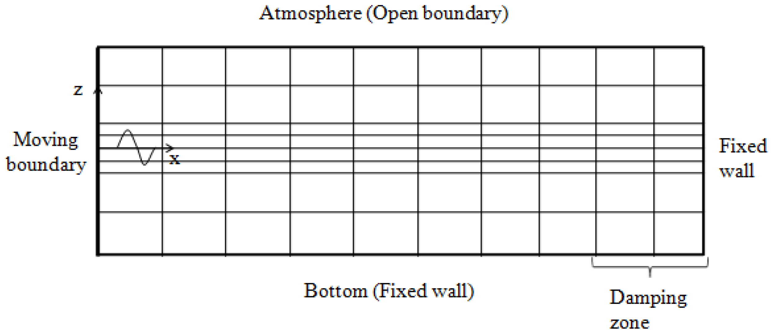
2. Numerical Model
2.1. Two-Phase Flow Model Description
2.2. Solving Procedure
- (1)
- Calculation of the time step based on Courant number;
- (2)
- Update of the dynamic meshes;
- (3)
- Update of the fluid properties (i.e., density ρ and dynamic viscosity μ);
- (4)
- Solving of Equation (3) by the MULES method to update the volume fraction function α;
- (5)
- Calculation of the velocity and pressure fields by the PISO algorithm.
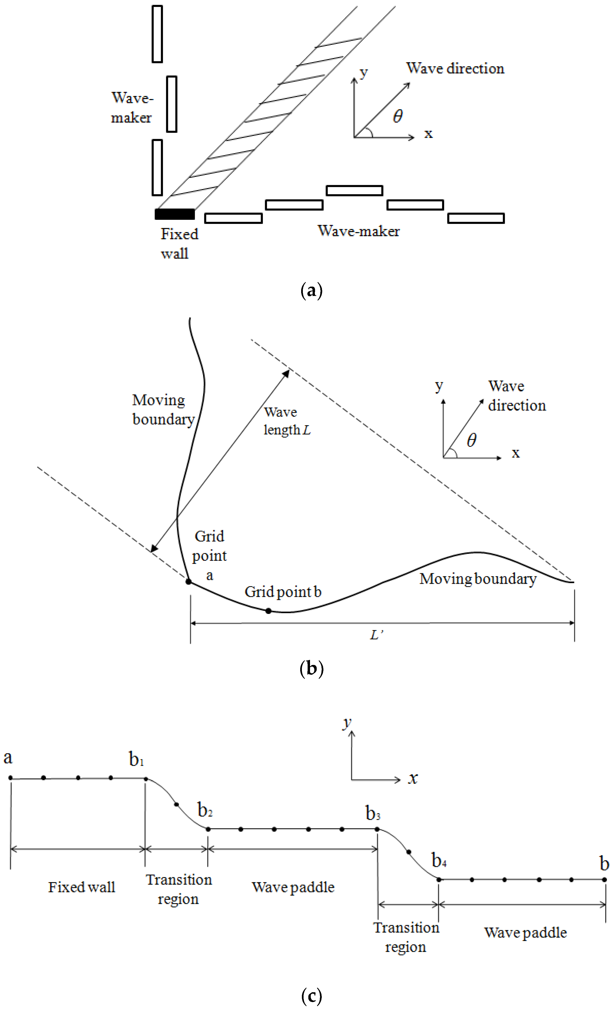
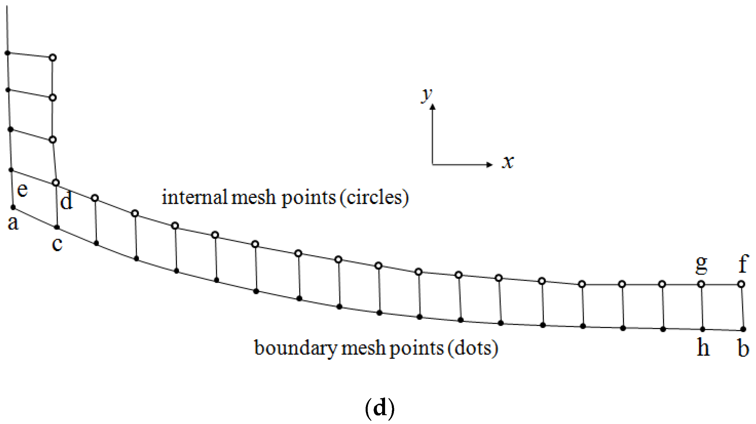
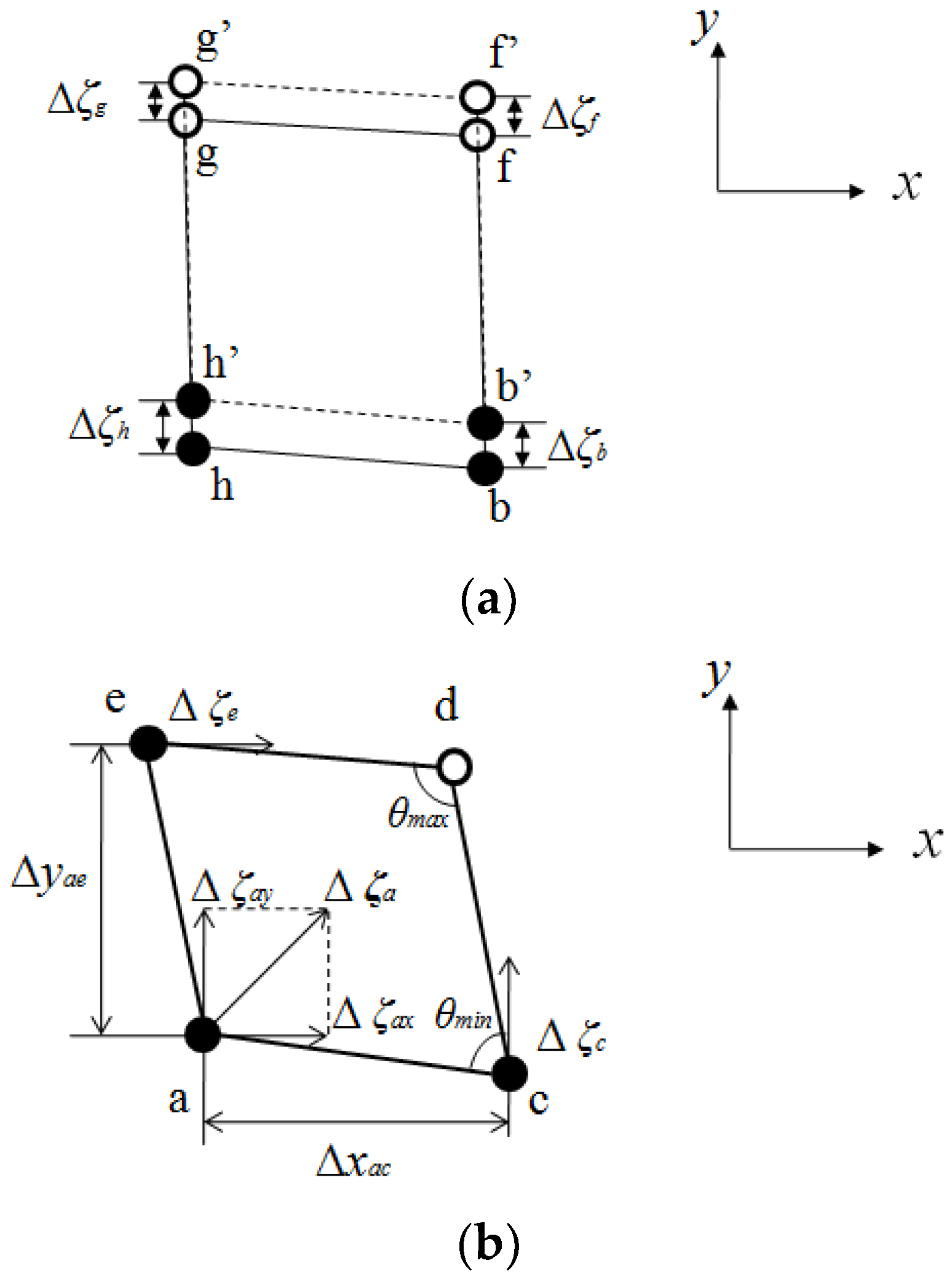
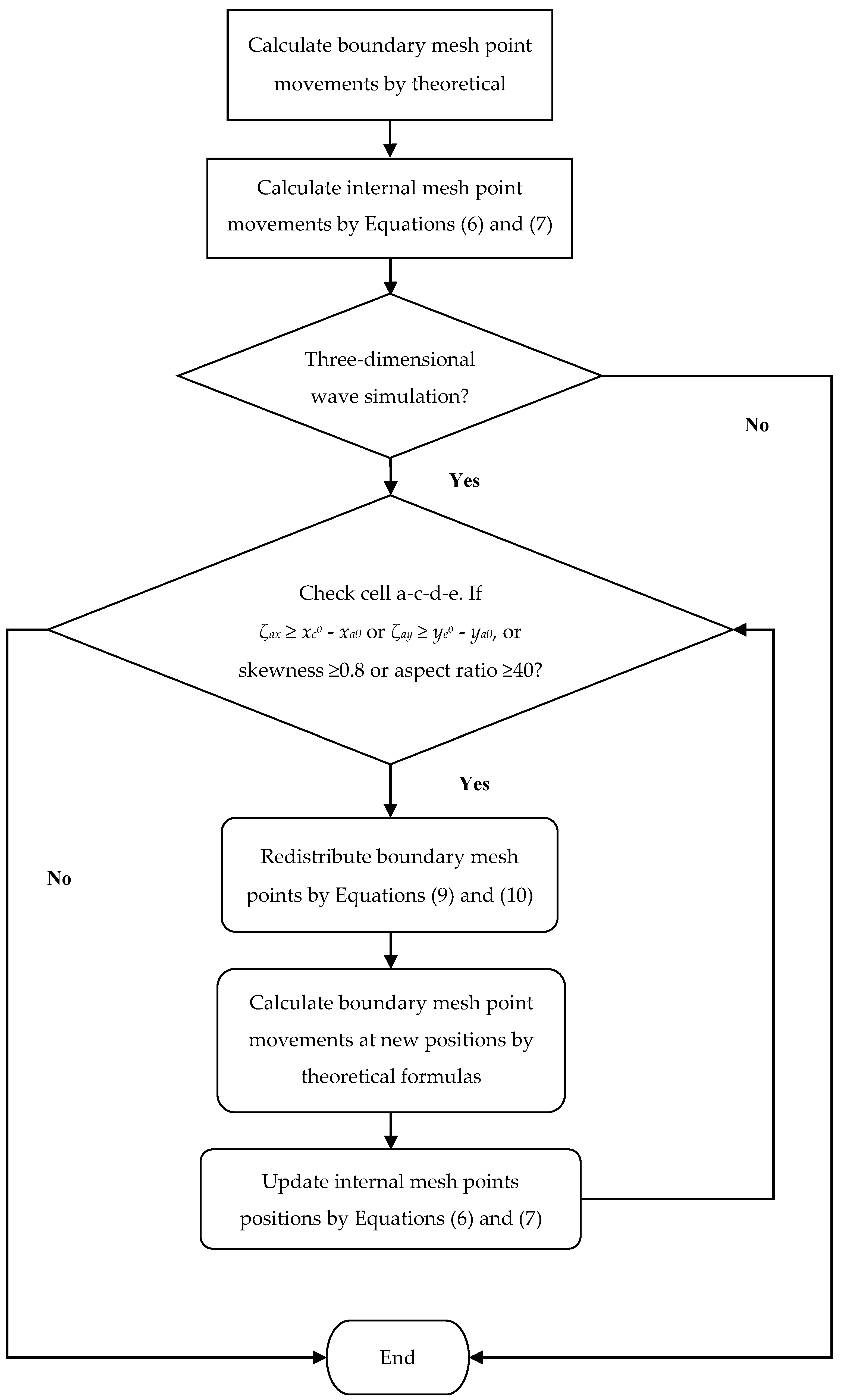
2.3. Wave Generation Based on the Moving Boundary Method
2.4. Wave Damping
2.5. Boundary Conditions
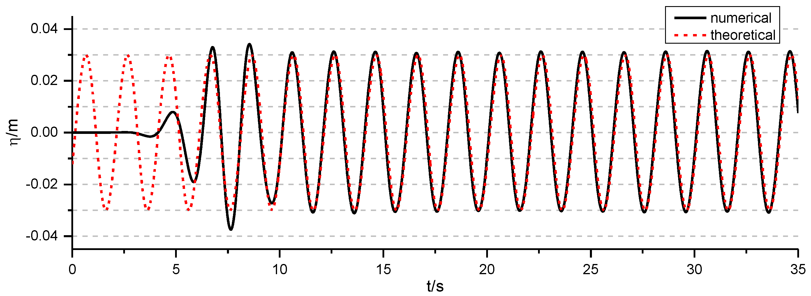
3. Two-Dimensional Regular Wave Simulation
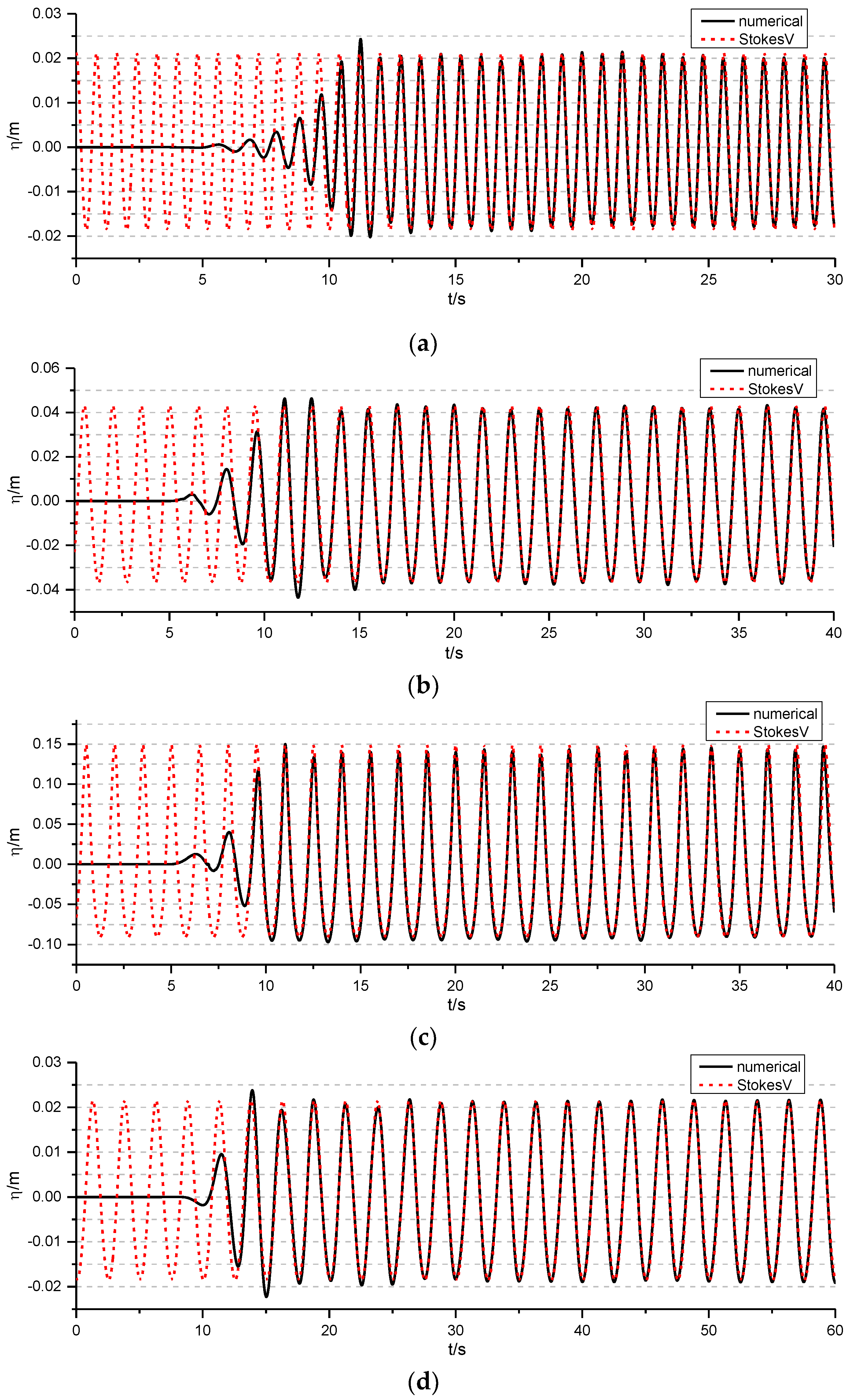
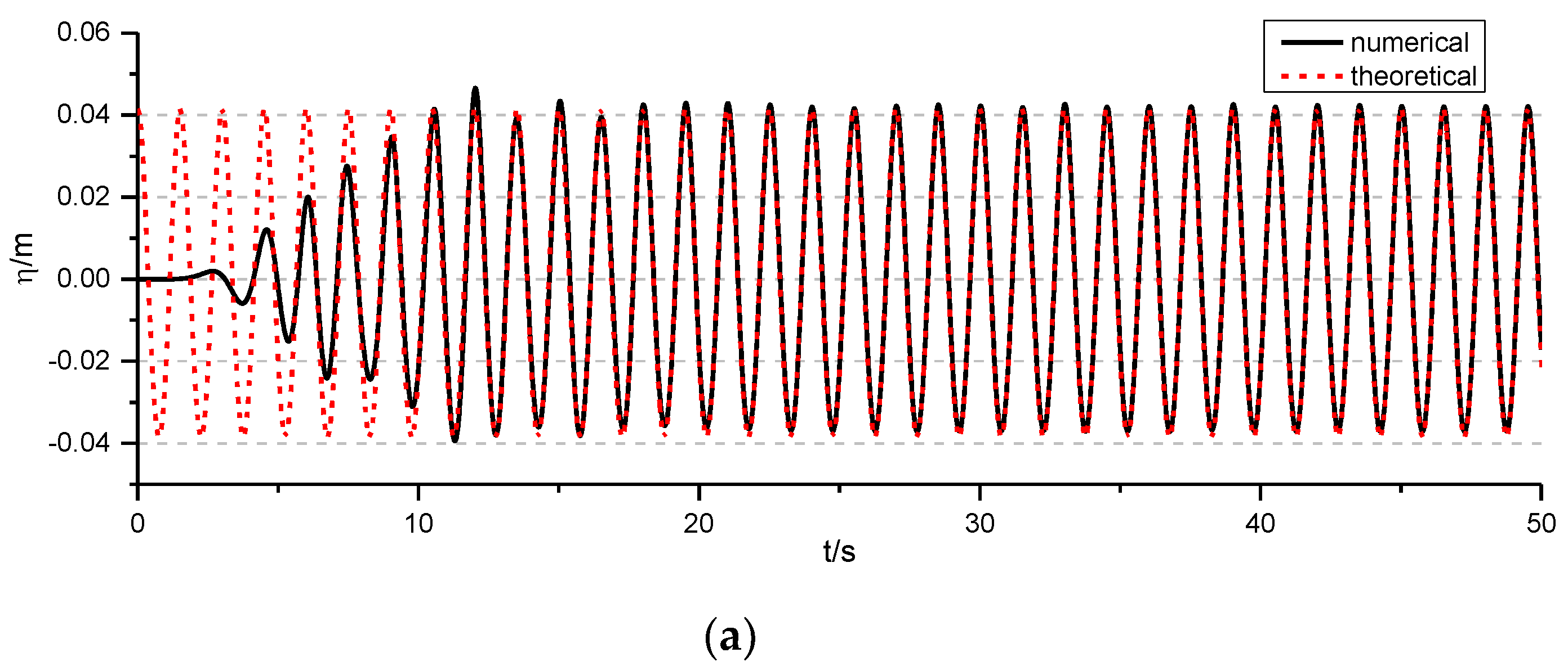
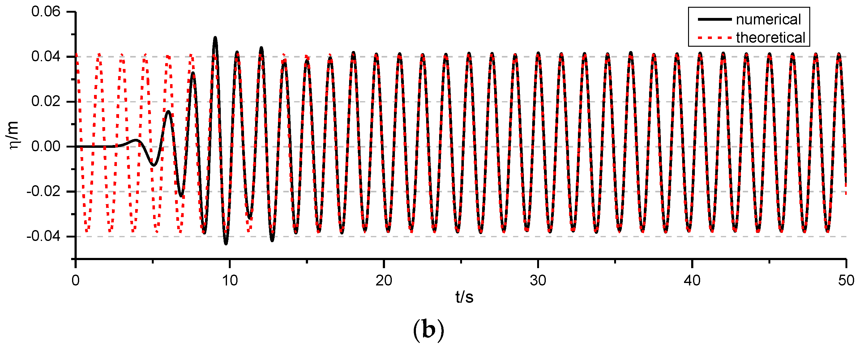
3.1. Wave Generation
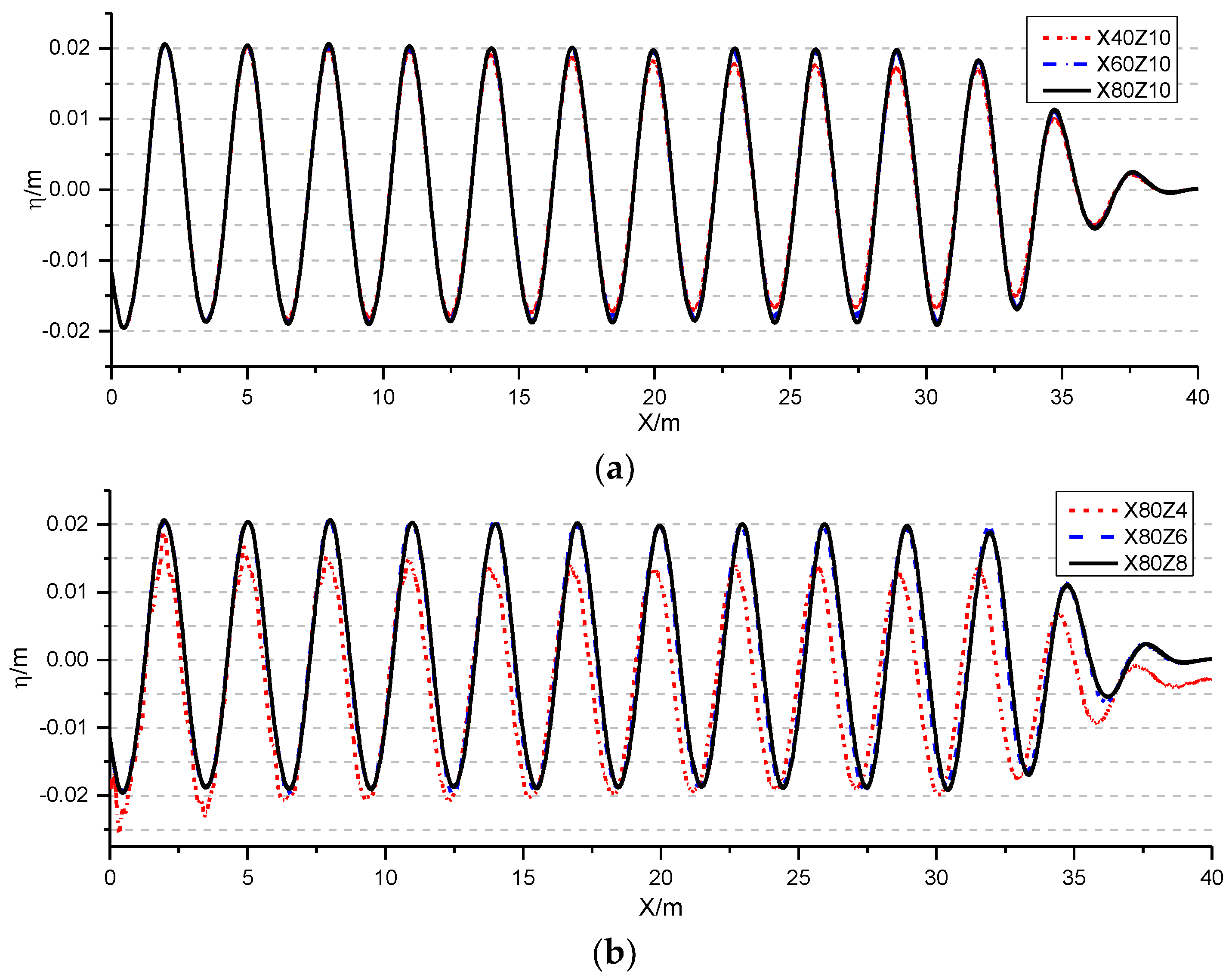
3.2. Mesh Convergence Study
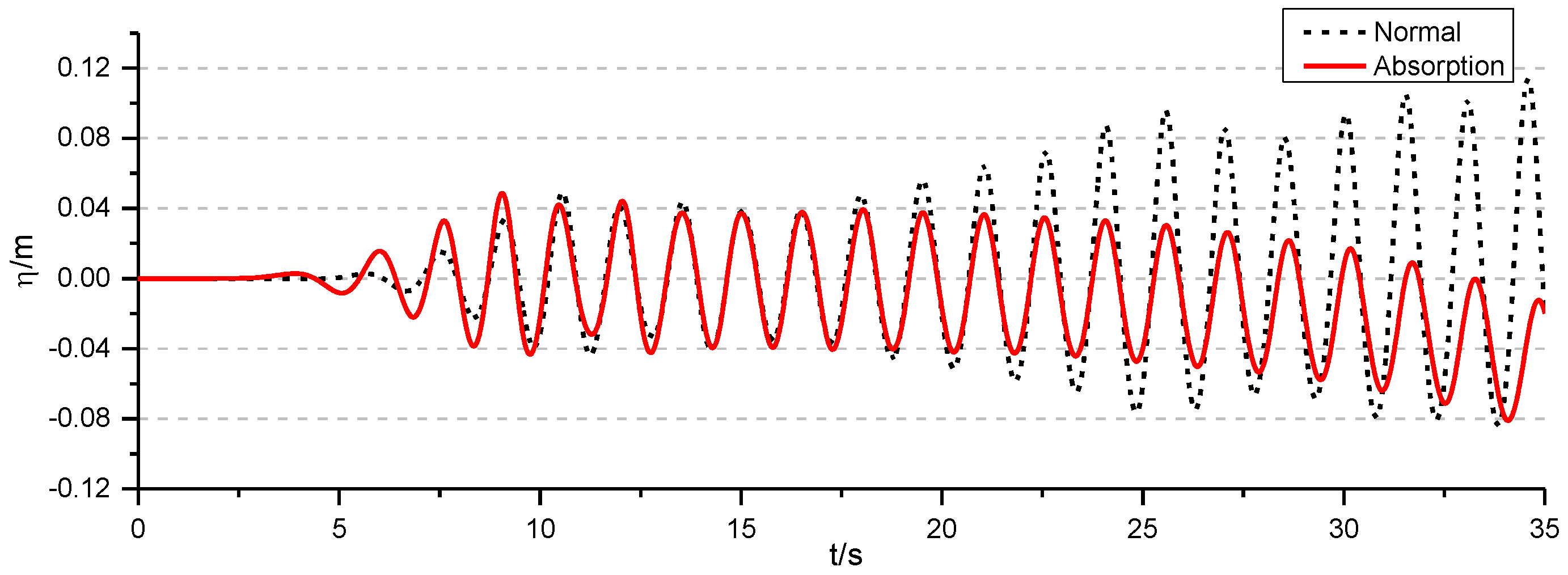
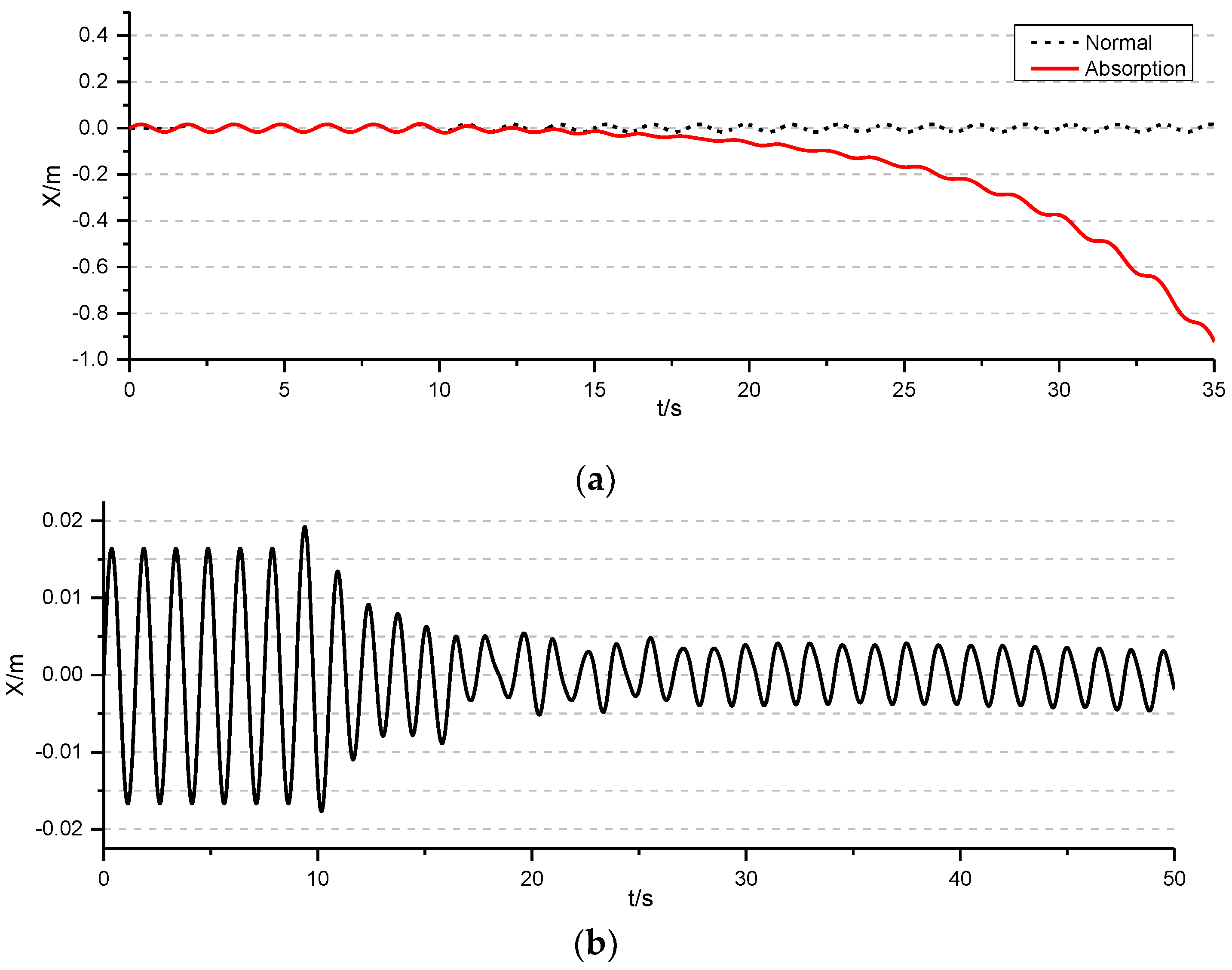
3.3. Active Wave Absorption
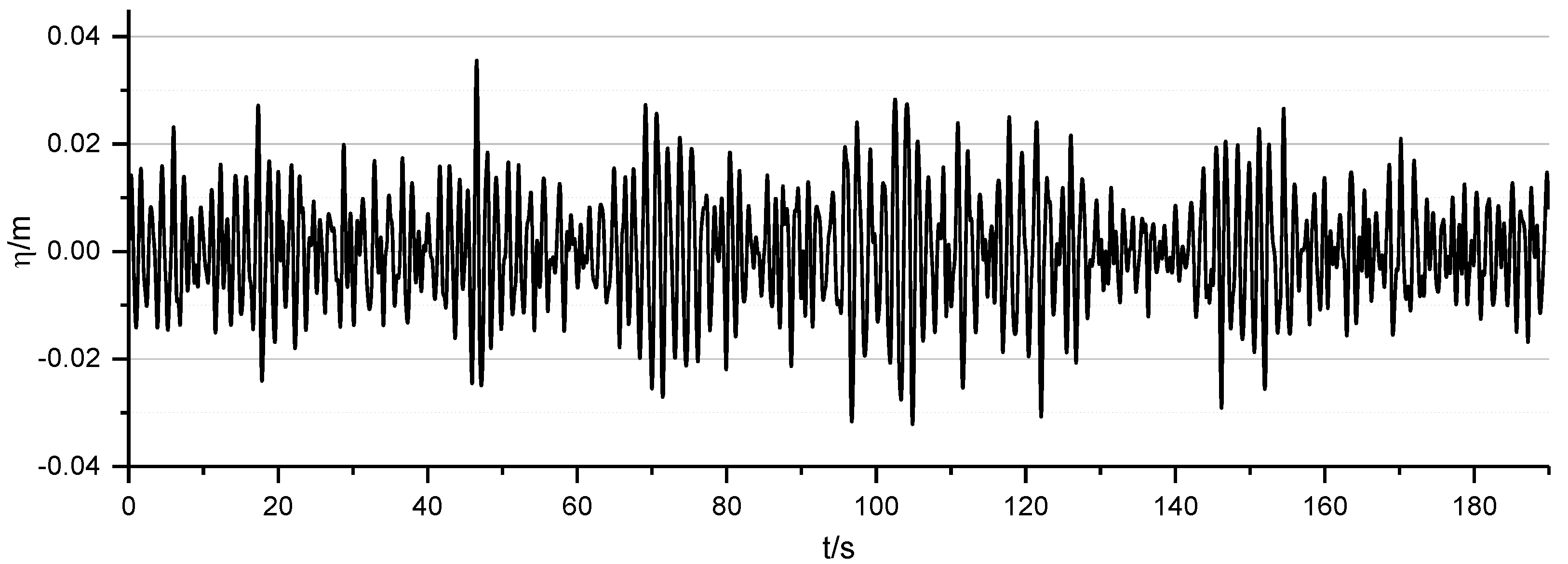
4. Two-Dimensional Irregular Wave Simulation
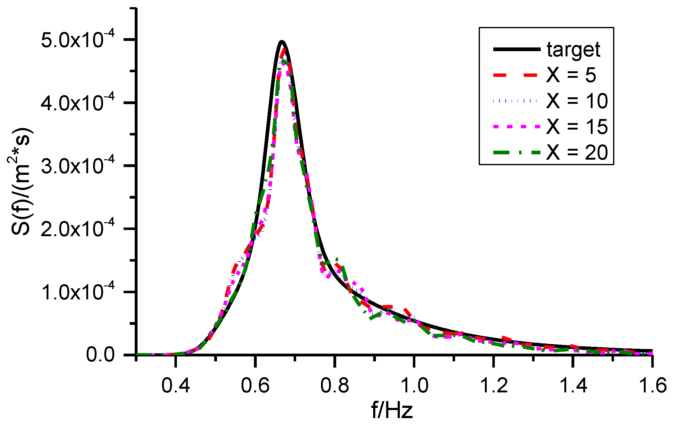
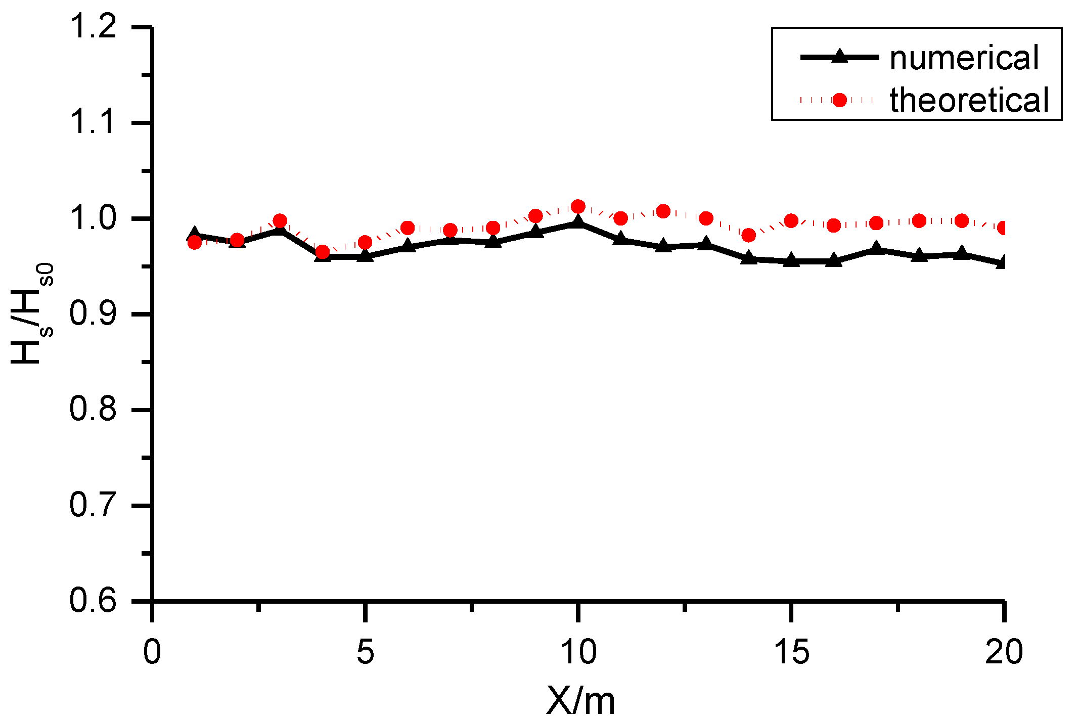
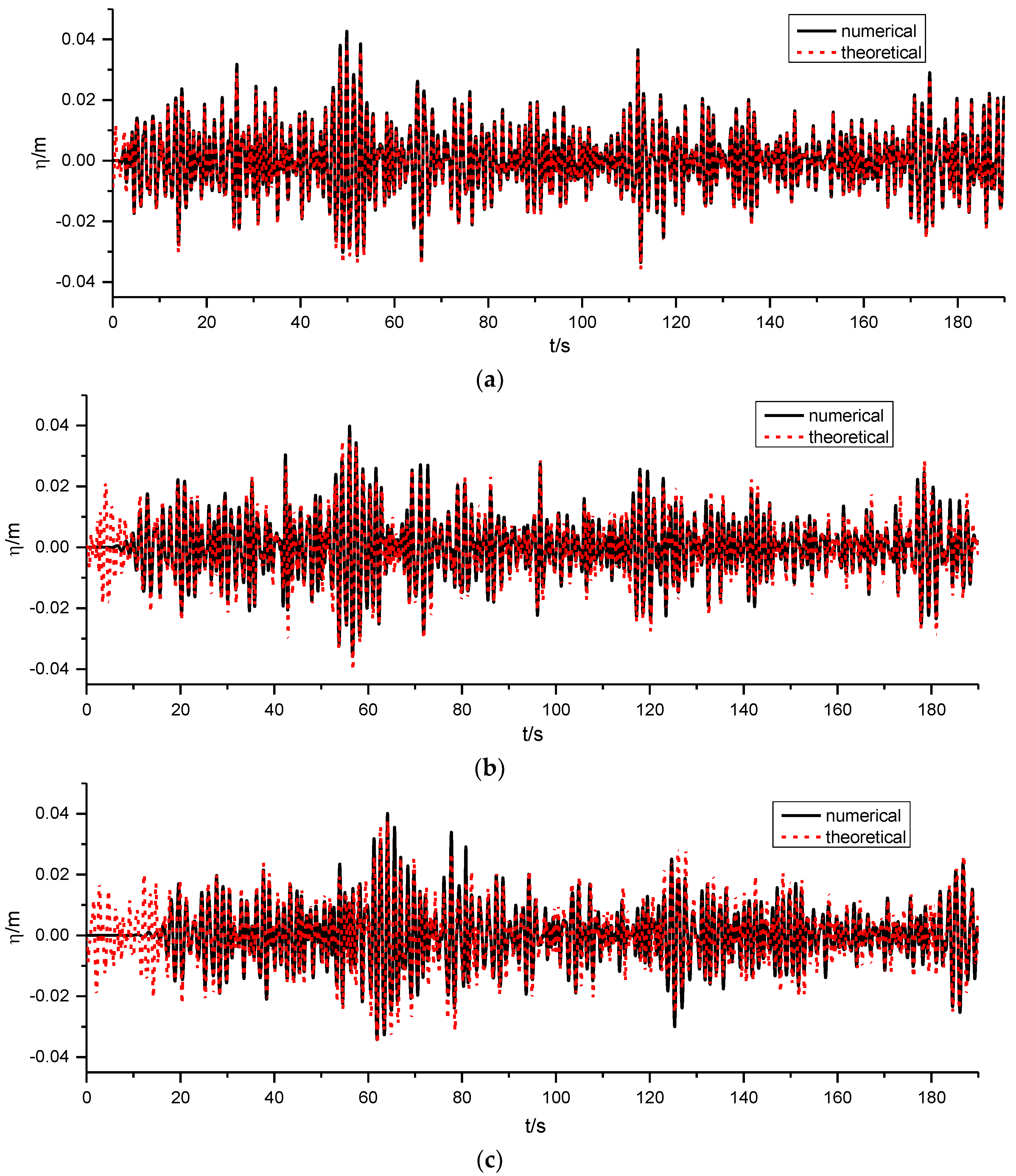
4.1. Wave Generation
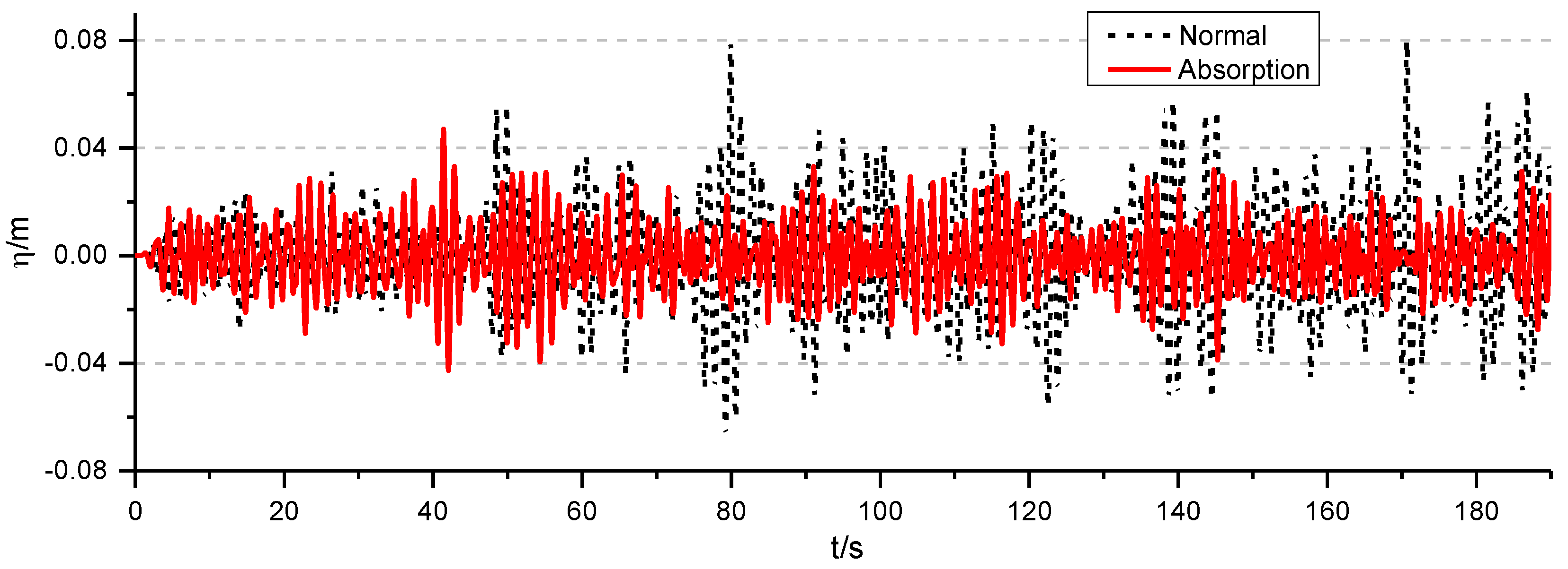
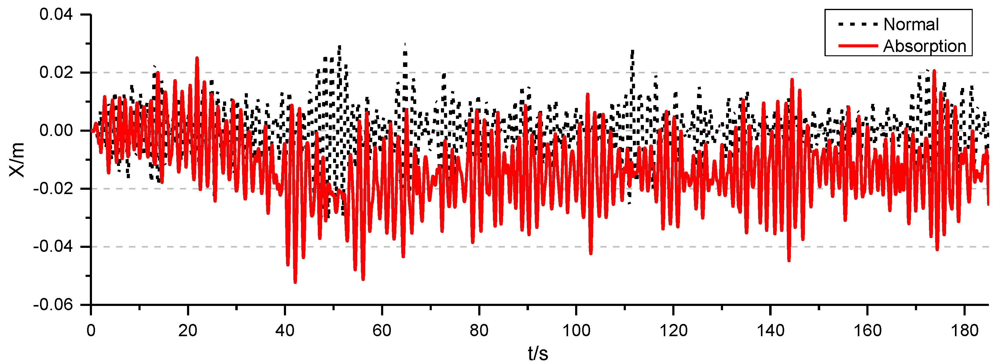
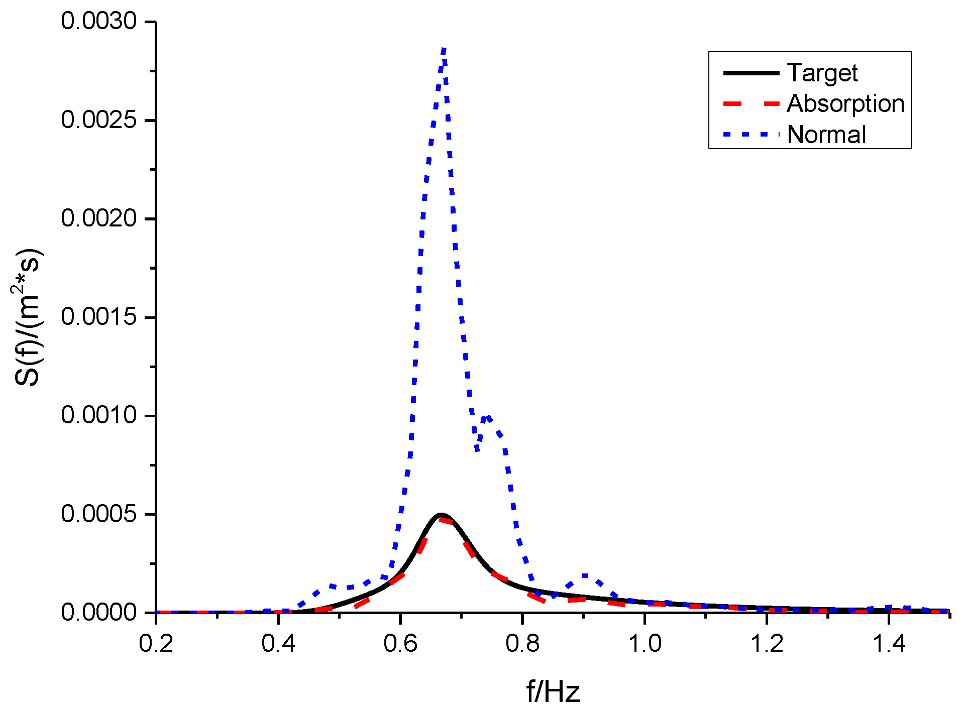
4.2. Active Wave Absorption
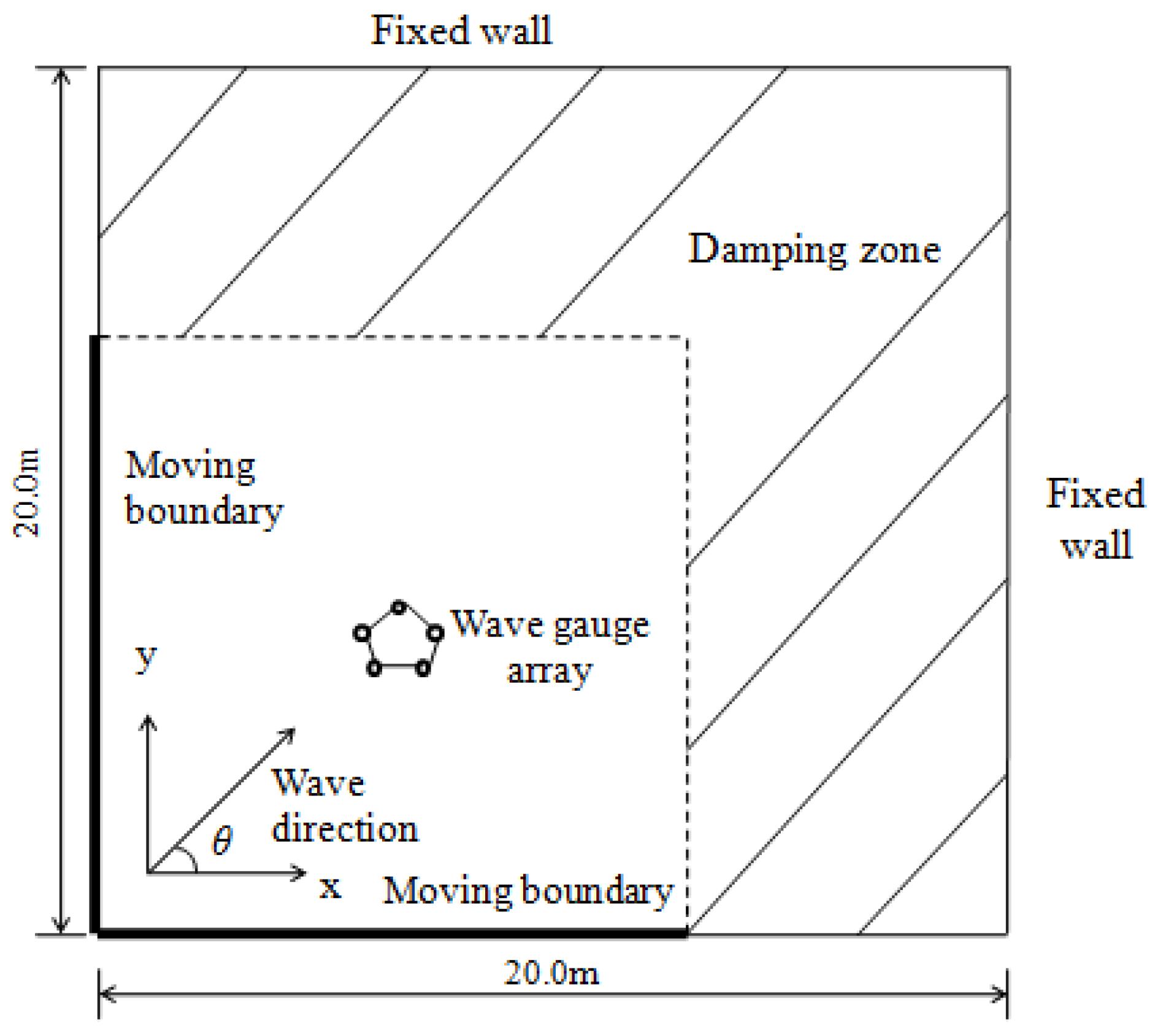
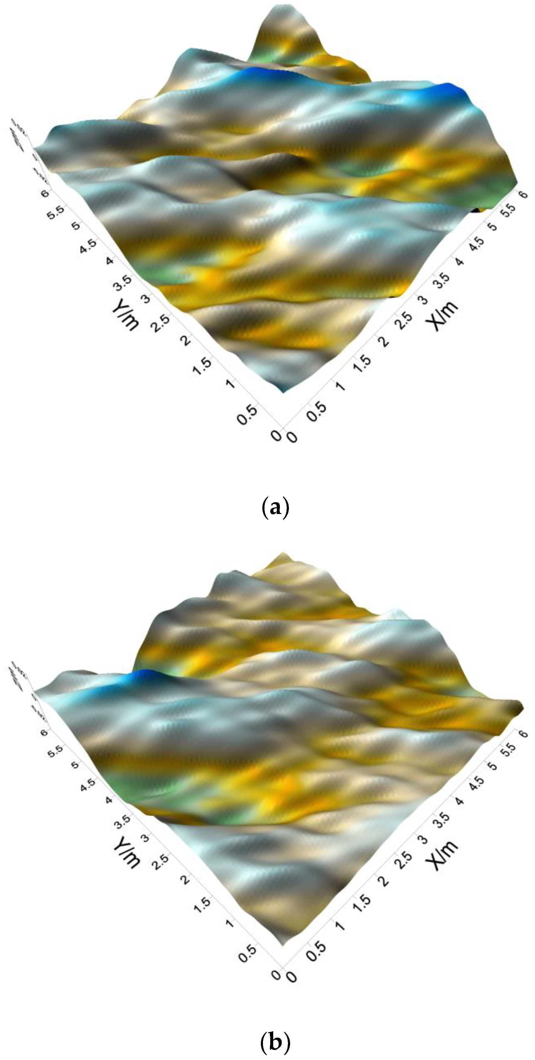
5. Three-Dimensional Wave Simulation
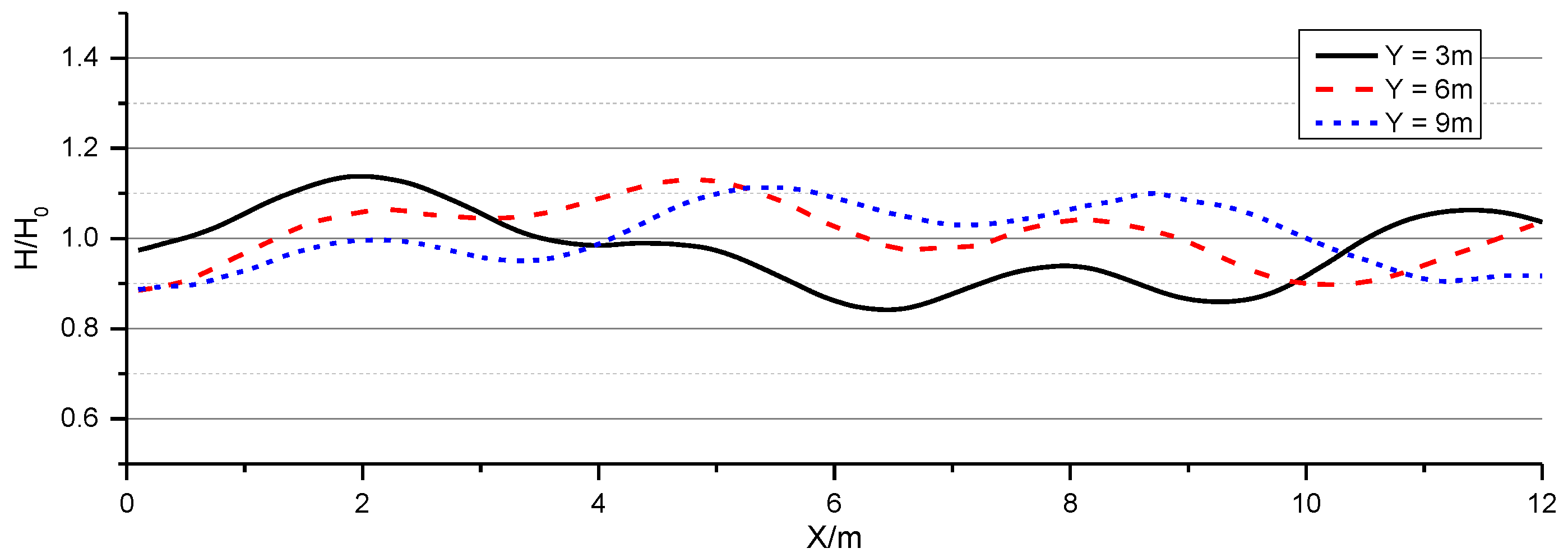
5.1. Oblique Regular Wave Generation
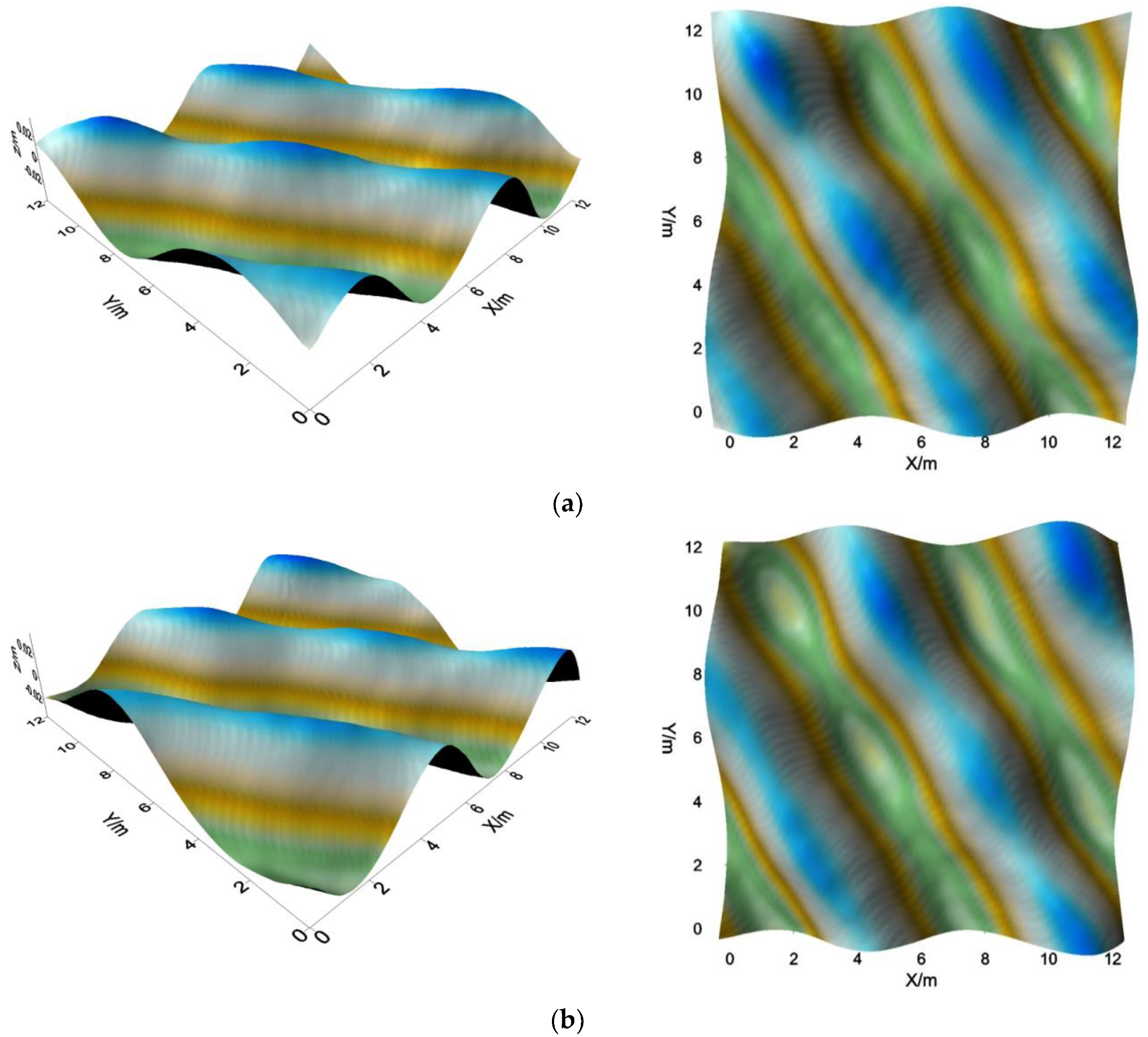
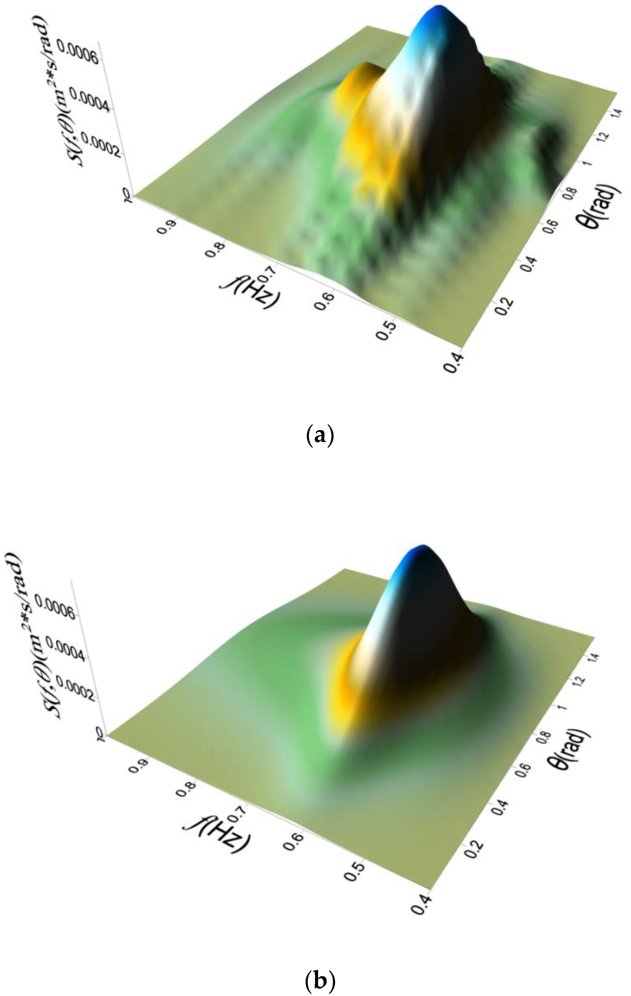
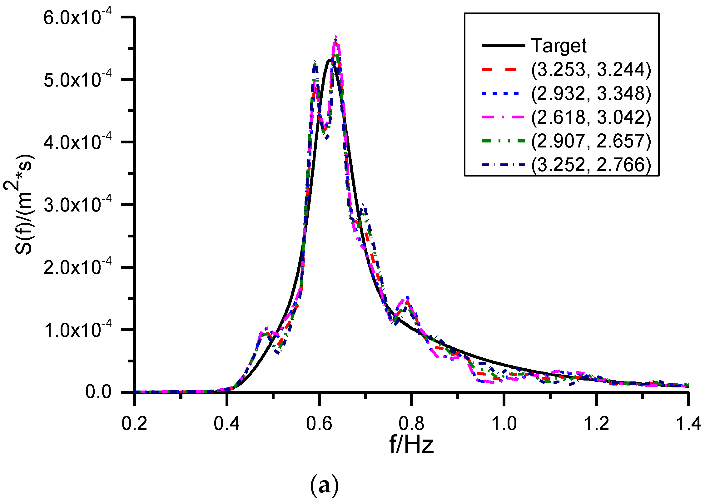
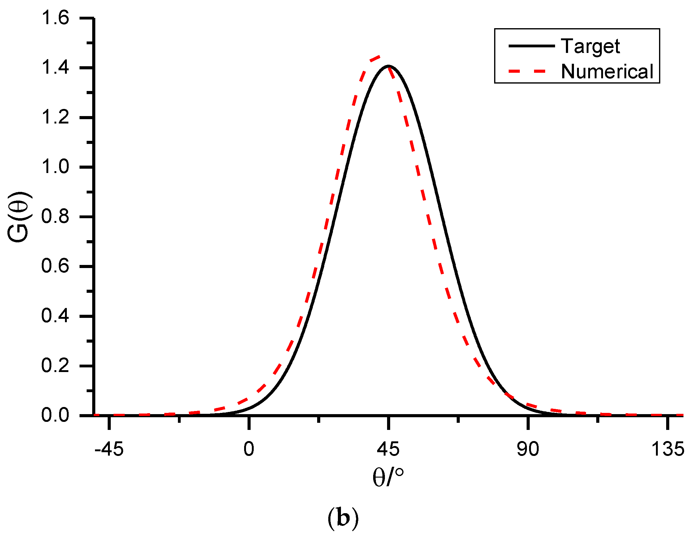
5.2. Multidirectional Random Wave Generation
6. Conclusions and Remarks
Author Contributions
Funding
Conflicts of Interest
References
- Lin, P.Z.; Liu, P.L.F. A numerical study of breaking waves in the surf zone. J. Fluid Mech. 1998, 359, 239–264. [Google Scholar] [CrossRef]
- Troch, P.; Rouck, J.D. An active wave generating—Absorbing boundary condition for VOF type numerical model. Coast. Eng. 1999, 38, 223–247. [Google Scholar] [CrossRef]
- Choi, B.H.; Dong, C.K.; Pelinovsky, E.; Woo, S.B. Three-dimensional simulation of tsunami run-up around conical island. Coast. Eng. 2007, 54, 618–629. [Google Scholar] [CrossRef]
- Cheng, Y.Z.; Jiang, C.B.; Wang, Y.Y. A coupled numerical model of wave interaction with porous medium. Ocean Eng. 2009, 36, 952–959. [Google Scholar] [CrossRef]
- Del Jesus, M.; Lara, J.L.; Losada, I.J. Three-dimensional interaction of waves and porous coastal structures: Part I: Numerical model formulation. Coast. Eng. 2012, 64, 57–72. [Google Scholar] [CrossRef]
- Jacobsen, N.G.; Fuhrman, D.R.; Fredsøe, J. A wave generation toolbox for the open-source CFD library: OpenFoam®. Int. J. Numer. Methods Fluids 2012, 70, 1073–1088. [Google Scholar] [CrossRef]
- Higuera, P.; Lara, J.L.; Losada, I.J. Realistic wave generation and active wave absorption for Navier-Stokes models: Application to OpenFOAM®. Coast. Eng. 2013, 71, 102–118. [Google Scholar] [CrossRef]
- Zhang, J.S.; Zhang, Y.; Jeng, D.S.; Liu, L.F.; Zhang, C. Numerical simulation of wave—Current interaction using a RANS solver. Ocean Eng. 2014, 75, 157–164. [Google Scholar] [CrossRef]
- Lin, P.Z.; Liu, P.L.F. Internal wave-maker for Navier-Stokes equations models. J. Waterw. Port Coast. Ocean Eng. 1999, 125, 207–215. [Google Scholar] [CrossRef]
- Ha, T.; Lin, P.Z.; Cho, Y.S. Generation of 3D regular and irregular waves using Navier-Stokes equations model with an internal wave maker. Coast. Eng. 2013, 76, 55–67. [Google Scholar] [CrossRef]
- Orszaghova, J.; Borthwick, A.G.L.; Taylor, P.H. From the paddle to the beach—A Boussinesq shallow water numerical wave tank based on Madsen and Sørensen’s equations. J. Comput. Phys. 2012, 231, 328–344. [Google Scholar] [CrossRef]
- Higuera, P.; Losada, I.J.; Lara, J.L. Three-dimensional numerical wave generation with moving boundaries. Coast. Eng. 2015, 101, 35–47. [Google Scholar] [CrossRef]
- Patankar, S.V.; Spalding, D.B. A calculation procedure for heat, mass and momentum transfer in three-dimensional parabolic flows. Int. J. Heat Mass Transf. 1972, 15, 1787–1806. [Google Scholar] [CrossRef]
- Issa, R.I. Solution of the implicitly discretised fluid flow equations by operator-splitting. J. Comput. Phys. 1991, 62, 40–65. [Google Scholar] [CrossRef]
- Jasak, H. Error Analysis and Estimation for the Finite Volume Method with Applications to Fluid Flows. Ph.D. Thesis, Imperial College London, London, UK, 1996. [Google Scholar]
- Rudman, M. Volume-Tracking Methods for Interfacial Flow Calculations. Int. J. Numer. Methods Fluids 1997, 24, 671–691. [Google Scholar] [CrossRef]
- Boris, J.P.; Book, D.L. Flux-corrected transport. I. SHASTA, a fluid transport algorithm that works. J. Comput. Phys. 1973, 11, 38–69. [Google Scholar] [CrossRef]
- Behr, M.; Tezduyar, T.E. Finite element solution strategies for large-scale flow simulations. Comput. Methods Appl. Mech. Eng. 1994, 112, 3–24. [Google Scholar] [CrossRef]
- Batina, J.T. Unsteady Euler airfoil solutions using unstructured dynamic meshes. AIAA J. 1990, 28, 1381–1388. [Google Scholar] [CrossRef]
- Löhner, R.; Yang, C. Improved ALE mesh velocities for moving bodies. Int. J. Numer. Methods Biomed. 1996, 12, 599–608. [Google Scholar] [CrossRef]
- Fluent Inc. Fluent User’s Guide; Fluent Inc.: Lebanon, NH, USA, 2003. [Google Scholar]
- Han, P. The Study of Damping Absorber for Irregular Waves Based on VOF Method. Master’s Thesis, Dalian University of Technology, Dalian, China, 2008. (In Chinese). [Google Scholar]
- Havelock, T.H. Forced surface-waves on water. Philos. Mag. 1929, 8, 569–576. [Google Scholar] [CrossRef]
- Fenton, J.D. A Fifth-Order Stokes Theory for Steady Waves. J. Waterw. Port Coast. Ocean Eng. 1985, 3, 216–234. [Google Scholar] [CrossRef]
- Méhauté, B.L. An Introduction to Hydrodynamics and Water Waves; Springer: New York, NY, USA, 1976. [Google Scholar]
- Willmott, C.J.; Ackleson, S.G.; Davis, R.E.; Feddema, J.J.; Klink, K.M.; Legates, D.R.; O’donnell, J.; Rowe, C.M. Statistics for the evaluation and comparison of models. J. Geophys. Res. Oceans 1985, 90, 8995–9005. [Google Scholar] [CrossRef]
- Goda, Y.; Suzuki, Y. Estimation of incident and reflected waves in random wave experiments. Coast. Eng. 1976, 4, 828–845. [Google Scholar] [CrossRef]
- Schäffer, H.A.; Klopman, G. Review of multidirectional active wave absorption methods. J. Waterw. Port Coast. Ocean Eng. 2000, 126, 88–97. [Google Scholar] [CrossRef]
- Hirakuchi, H.; Kajima, R.; Kawaguchi, T. Application of a piston-type absorbing wavemaker to irregular wave experiments. Coast. Eng. Jpn. 1990, 33, 11–24. [Google Scholar] [CrossRef]
- Liu, S.X.; Wang, X.T.; Li, M.G.; Guo, M.Y. Active Absorption Wave Maker System for Irregular Waves. China Ocean Eng. 2003, 17, 203–214. [Google Scholar]
- Zhang, H.W.; Schäffer, H.A.; Jakobsen, K.P. Deterministic combination of numerical and physical coastal wave models. Coast. Eng. 2007, 54, 171–186. [Google Scholar] [CrossRef]
- Goda, Y. A comparative review on the functional forms of directional wave. Coast. Eng. J. 1999, 41, 1–20. [Google Scholar] [CrossRef]
- Takayama, T. Theoretical properties of oblique waves generated by serpent-type wave-makers. Rep. Port Harb. Res. Inst. 1982, 21, 3–47. [Google Scholar]
- Zhou, Z. Theoretical Studies for the Properties of Waves Generated by Segment Wavemakers. Master’s Thesis, Dalian University of Technology, Dalian, China, 2016. (In Chinese). [Google Scholar]
- Yu, Y.X.; Liu, S.X.; Li, L. Numerical Simulation of Multi-Directional Random Seas. China Ocean Eng. 1991, 5, 311–320. [Google Scholar]
- Hashimoto, N.; Kobune, K.; Kameyama, Y. Estimation of directional spectrum using the Bayesian approach and its application to filed data analysis. Rep. Port Harb. Res. Inst. 1987, 26, 57–100. [Google Scholar]


| Case | Water Depth d(m) | Wave Height H(m) | Wave Period T(s) | Wave Length L(m) | L/∆x | H/∆y | ∆x/∆y |
|---|---|---|---|---|---|---|---|
| 1 | 0.60 | 0.04 | 0.80 | 1.00 | 149.96 | 8.00 | 1.33 |
| 2 | 0.60 | 0.08 | 1.50 | 2.99 | 149.50 | 6.00 | 1.50 |
| 3 | 0.60 | 0.24 | 1.50 | 2.99 | 99.64 | 8.00 | 1.00 |
| 4 | 0.60 | 0.04 | 2.50 | 5.67 | 100.02 | 8.00 | 11.34 |
| Case | 1 | 2 | 3 | 4 |
|---|---|---|---|---|
| Root-mean-square error | 0.00199 | 0.00253 | 0.00887 | 0.00081 |
| Case | 1 | 2 | 3 | 4 |
|---|---|---|---|---|
| Reflection coefficients | 5.1% | 3.8% | 10.9% | 3.1% |
| Position (m) | 1 | 10 | 20 |
|---|---|---|---|
| Root-mean-square error | 0.00092 | 0.00371 | 0.00491 |
© 2020 by the authors. Licensee MDPI, Basel, Switzerland. This article is an open access article distributed under the terms and conditions of the Creative Commons Attribution (CC BY) license (http://creativecommons.org/licenses/by/4.0/).
Share and Cite
Jia, W.; Liu, S.; Li, J.; Fan, Y. A Three-Dimensional Numerical Model with an L-Type Wave-Maker System for Water Wave Simulations by the Moving Boundary Method. Water 2020, 12, 161. https://doi.org/10.3390/w12010161
Jia W, Liu S, Li J, Fan Y. A Three-Dimensional Numerical Model with an L-Type Wave-Maker System for Water Wave Simulations by the Moving Boundary Method. Water. 2020; 12(1):161. https://doi.org/10.3390/w12010161
Chicago/Turabian StyleJia, Wei, Shuxue Liu, Jinxuan Li, and Yuping Fan. 2020. "A Three-Dimensional Numerical Model with an L-Type Wave-Maker System for Water Wave Simulations by the Moving Boundary Method" Water 12, no. 1: 161. https://doi.org/10.3390/w12010161
APA StyleJia, W., Liu, S., Li, J., & Fan, Y. (2020). A Three-Dimensional Numerical Model with an L-Type Wave-Maker System for Water Wave Simulations by the Moving Boundary Method. Water, 12(1), 161. https://doi.org/10.3390/w12010161