Article

Flash Flood Forecasting Based on Long Short-Term Memory Networks

School of Hydraulic Engineering, Dalian University of Technology, Dalian 116024, China
*
Author to whom correspondence should be addressed.
Water 2020, 12(1), 109; https://doi.org/10.3390/w12010109
Submission received: 28 November 2019 / Revised: 21 December 2019 / Accepted: 27 December 2019 / Published: 29 December 2019
(This article belongs to the Section Hydrology)

Abstract

:
Flash floods occur frequently and distribute widely in mountainous areas because of complex geographic and geomorphic conditions and various climate types. Effective flash flood forecasting with useful lead times remains a challenge due to its high burstiness and short response time. Recently, machine learning has led to substantial changes across many areas of study. In hydrology, the advent of novel machine learning methods has started to encourage novel applications or substantially improve old ones. This study aims to establish a discharge forecasting model based on Long Short-Term Memory (LSTM) networks for flash flood forecasting in mountainous catchments. The proposed LSTM flood forecasting (LSTM-FF) model is composed of T multivariate single-step LSTM networks and takes spatial and temporal dynamics information of observed and forecast rainfall and early discharge as inputs. The case study in Anhe revealed that the proposed models can effectively predict flash floods, especially the qualified rates (the ratio of the number of qualified events to the total number of flood events) of large flood events are above 94.7% at 1–5 h lead time and range from 84.2% to 89.5% at 6–10 h lead-time. For the large flood simulation, the small flood events can help the LSTM-FF model to explore a better rainfall-runoff relationship. The impact analysis of weights in the LSTM network structures shows that the discharge input plays a more obvious role in the 1-h LSTM network and the effect decreases with the lead-time. Meanwhile, in the adjacent lead-time, the LSTM networks explored a similar relationship between input and output. The study provides a new approach for flash flood forecasting and the highly accurate forecast contributes to prepare for and mitigate disasters.

1. Introduction

Flash floods are among the most destructive natural disasters in many countries of the world and are characterized by widespread distribution, large quantities, and rapid occurrence. From 2005 to 2015, China had an average of one hundred flash flood events which caused casualties each year [1]. Distinguished from regular floods, flash floods often occur in mountainous catchments of a few hundred square kilometers with a few hours of evacuation time. Short lead time is largely attributed to the quick response of the rainfall-runoff relationship, which is impacted by not only complex geographic and geomorphic conditions but also rainfall intensity and spatial-temporal distribution [2]. In practice, numerous catchments are facing a tough challenge of flash flood forecasting around the world [3]. Accurate and reliable short-term discharge forecasting is of great significance to preventing or mitigating a flash flood disaster.
Establishing a practical real-time forecasting model is one of the major tasks in flash flood prevention. Hapuarachchi et al. [4] provided an extensive review of flash flood forecasting and concluded no model could make reliable flash flood forecasts in spite of the plausible results of physically-based distributed hydrological models. Many studies showed that distributed hydrological models have advantages over lumped hydrological models and data-driven models, but they are computationally inefficient and need high-resolution sophisticated input data (e.g., DEM, land-use and soil maps, and soil characteristics) [5]. Hence, their applicability is limited in mountainous catchments. The expected benefits of using high-resolution distributed models might be masked by the increasing uncertainties at small scales [6]. Lumped hydrological models for flash flood forecasting are limited by their coarse resolution and inadequate description of rainfall spatial distribution, which has a great impact on the catchment response [2]. In addition, physically-based hydrological models depend heavily on their boundary conditions, which are often poorly defined [7]. It is difficult to describe flash flood generation and propagation by a deterministic approach due to the complexity of its processes. Numerous studies indicate the gap of physically-based hydrological models in short-term flood prediction [8].
With the advancements in system theory and computer technology, Machine Learning (ML) has been widely used in hydrology, such as Artificial Neural Networks (ANN) [9], Adaptive Network-Based Fuzzy Inference System [10], Extreme Learning Machines [11], and so on [8,12]. Compared with hydrological models, data-driven models are able to obtain better or comparable forecasting results. Besides, they have fewer restrictions and assumptions on modeling, small computational costs and fast computation times [8,12]. However, the time series characteristic of hydrological forecasting is seldom considered by the internal structure of these models. Recurrent neural networks (RNNs) are specifically designed to deal with time series problems. Chang et al. [13] applied RNNs for urban flood control and found RNNs had higher applicability than ANNs. The most successful and widely used RNNs is the Long Short-Term Memory (LSTM) network. As a special type of RNN, the LSTM network is designed to overcome the drawback of the traditional RNN of learning long-term dependencies. It is regarded as a milestone in dealing with time series problems in machine learning.
LSTM was proposed by Hochreiter and Schmidhuber [14], later modified by Felix Gers in 2001 and promoted by Alex Graves in 2006. It has been widely used to analyze the time series in many applications like natural language processing, speech recognition, handwriting recognition, sentiment analysis as well as in disease diagnosis. Previous studies have shown that the LSTM model outperformed the conceptual and physical-based models for simulating the rainfall-runoff process [15], and is more stable than an ANN model in different lead-time modeling [16]. The LSTM model has an advantage over other ML approaches in capturing the time-series dynamics of discharges and reducing the time consumption and memory storage [17]. Moreover, LSTM also outperforms other neural networks in predicting water table depth in agricultural areas [18], monitoring sewer overflow [19], simulating the reservoir operation [17] and so on. To our knowledge, there has been no previous attempt to deploy the LSTM network on discharge forecasting in small mountainous catchments to assess its performance in flash flood forecasting.
The aim of this study is to propose a data-driven discharge forecasting model based on LSTM networks for flash flood forecasting in mountainous catchments. The LSTM model composed of T multivariate single-step LSTM networks with spatial and temporal dynamics information of rainfall and early discharge as inputs is established. The Anhe catchment is taken as a case study to validate the feasibility of the proposed model with the qualified rates of peak flow, lead-time, and the discharge hydrograph as the evaluation indexes. Moreover, the effects of the inputs and structure on the forecasts in different lead-times are analyzed through the parameter analysis.

2. Methodology

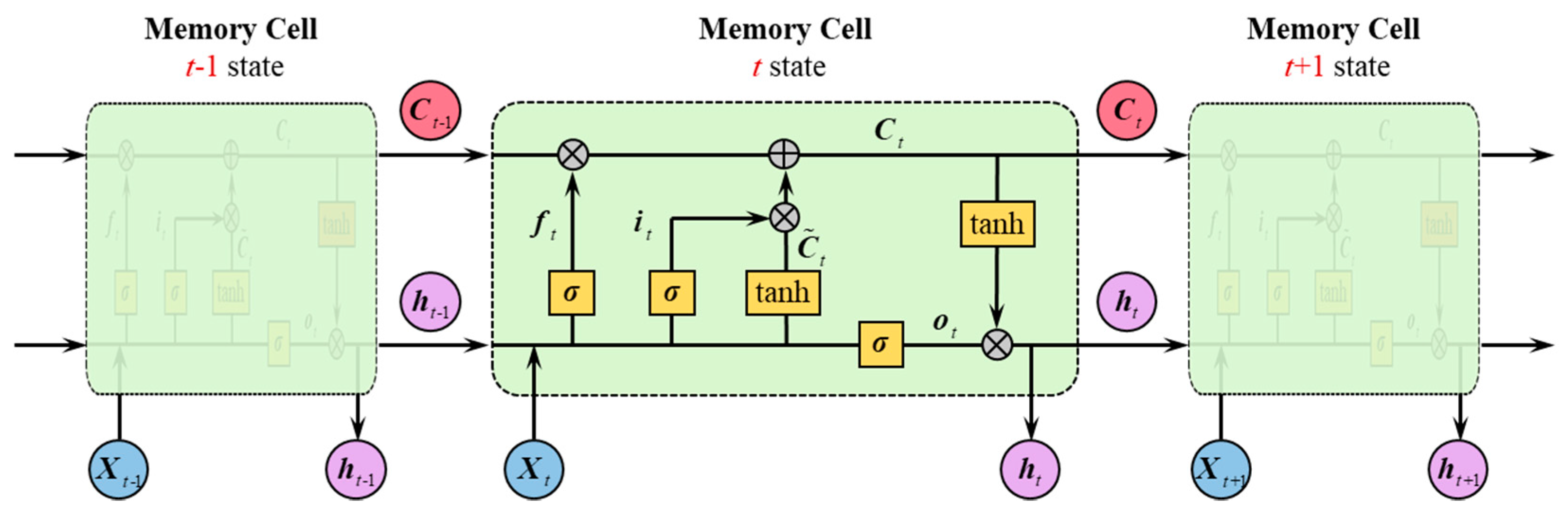
2.1. Long Short-Term Memory Network

LSTM is a special kind of RNN due to its structures called gates, which have the ability to remove or add information to the cell state. The LSTM memory cell has three gates to control the cell state. The input gate can allow the input signal to alter the state of the memory cell or block it. The output gate can allow or prevent the state of the memory cell to the output of the memory cell. The forget gate can allow the memory cell to remember or forget how much information to its next state. Figure 1 shows the internals of the LSTM memory cell and its relationship with adjacent time. The internal calculation process of the LSTM memory cell is shown in Equations (1)–(6).
f t = σ ( W f [ X t , h t 1 ] + b f )
i t = σ ( W i · [ X t ,   h t 1 ] + b i )
C ˜ t = tanh ( W c · [ X t ,   h t 1 ] + b c )
C t = f t C t 1 + i t C ˜ t
o t = σ ( W o · [ X t ,   h t 1 ] + b o )
h t = o t tanh ( C t )
where X t 1 ,   X t ,   X t + 1 and h t 1 ,   h t ,   h t + 1 are the input to the memory cell and hidden state at time t − 1, t, t + 1; C t 1 and C t are the cell state at time t − 1 and t; f t ,   i t ,   o t are the state of the forget gate, input gate and output gate; W f ,   W i ,   W o ,   W c and b f ,   b i ,   b o ,   b c are the weight matrices and bias vectors of the forget gate, input gate, output gate and calculating candidate state value C ˜ t , respectively; f t ,   i t ,   o t ,   h t and C ˜ t have the same dimension as C t . σ ( ) and tanh() presents the activation function of sigmoid() and tanh(), respectively. Sigmoid, with values in the range (0, 1), is used to express the switch state of the gate. Tanh(), with values in the range (−1, 1), is used to update the cell state and hidden state.

2.2. LSTM Flood Forecasting Model

The LSTM flood forecasting (LSTM-FF) model, composed of T multivariate single-step LSTM networks, is established to forecast discharge for 1 − T hour lead-time. As is shown in Figure 2, each discharge is forecasted by using a separated LSTM network. The inputs include (1) observations: a. current and previous (1 hour-lag, 2 hour-lag, …, H hour-lag) observed rainfall at each rain station, b. previous discharge at the outlet; and (2) forecasts: short-term forecast rainfall with lead-time of T. The observed inputs are represented by X t H ,   ,   X t 1 ,   X t , while the forecasting inputs are represented by X t + 1 ,   X t + 2 ,   ,   X t + T . The outputs include forecast discharge q t + 1 s i m ,   q t + 2 s i m ,   ,   q t + T s i m . Rectified Linear Unit (ReLU) with values in the range (0, +∞) is used to output non-negative values.
The model training steps are as follows.
Step 1:
Determine the discharge lead-time T according to the practical requirement for flash flood early warning in the specific catchment.
Step 2:
Establish and normalize the data set. Since rainfall and discharge have different physical significance and dimensions, the data is normalized with Equation (7).
x ^ = x x m i n x m a x x m i n
where x ^ is the normalized value; x is the observed value; x m a x and x m i n are the maximum and minimum observed values.
Step 3:
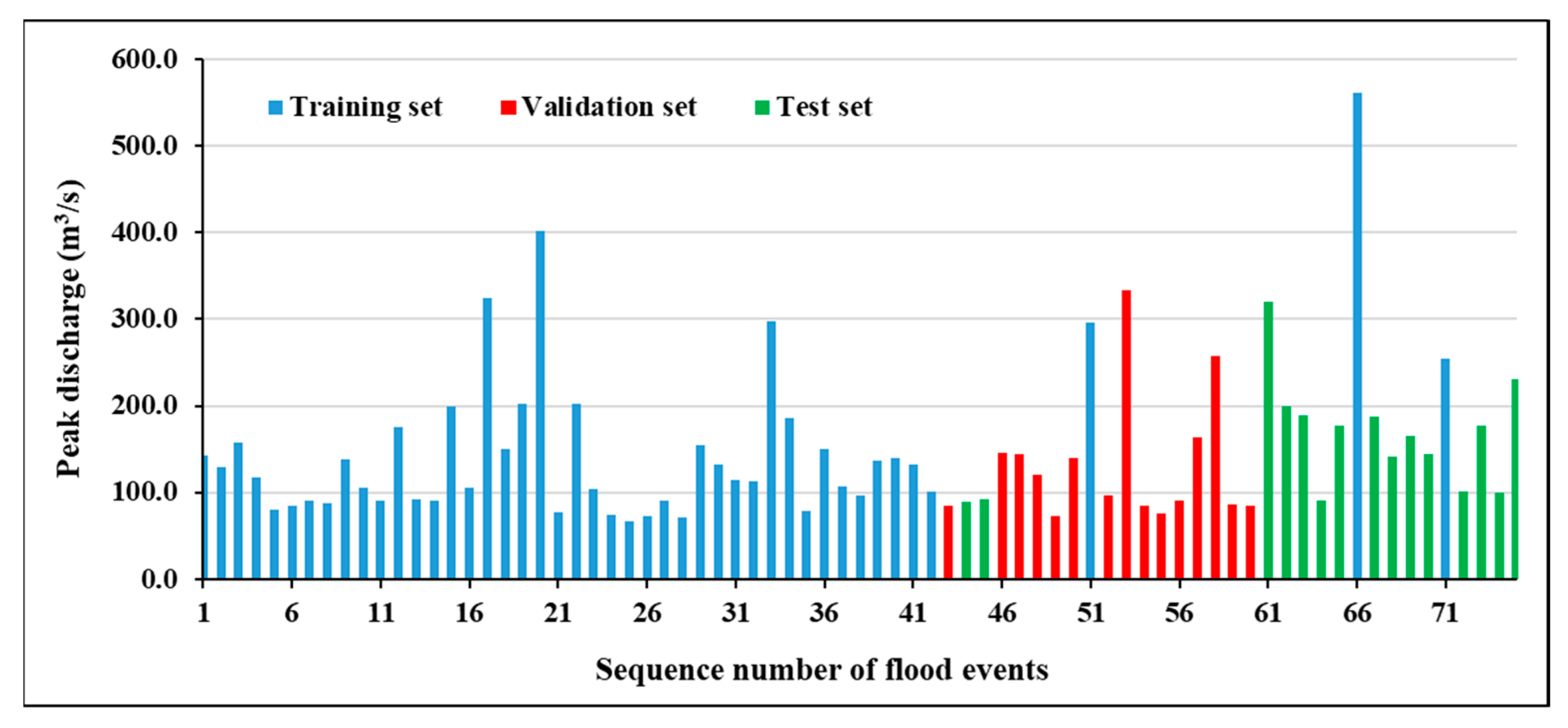
Divide the data set into the training set, validation set, and test set.
Step 4:
Give an initial value of hyperparameters (units, batch-size, and epoch) and train the 1-h, 2-h, …, T-hour LSTM networks, respectively. Units represent the dimensions of C t and h t . Batch-size defines the number of samples that will be propagated through the network. An epoch indicates the number of passes through the entire training dataset the machine learning algorithm has completed. If the batch-size is the whole training dataset, then batch size and epoch are equivalent. The initialization of weights is implemented by a random seed, which is determined by trial and error.
Step 5:
Repeat step 4 by trial and error, and determine the final value of hyperparameters for 1-h, 2-h, …, T-hour LSTM networks, respectively. The learning curve is used to prevent overfitting or underfitting.
Step 6:
Save the optimal model on the basis of the trial-and-error results in step 6.
Step 7:
Input test set to the saved LSTM-FF model and anti-normalize the output to simulated discharges.
Step 8:
Evaluate the simulated results of the LSTM-FF model.

2.3. Evaluation Criteria

The following error statistics and goodness of fit measures were adopted in this study.
(1) Relative Peak Error (RPE)
Forecasting the peak discharge (or rising stage) accurately is the primary task in flash flood prevention. Due to the characteristic of a steep rise in flash floods, a high prediction accuracy of peak discharge also means a relatively higher accuracy of peak time and flood hydrograph, especially for floods with high peak discharge. In this paper, RPE, defined by the following Equation, is taken as the main accuracy evaluation index.
R P E = q p e a k s i m q p e a k o b s q p e a k o b s × 100 %
where q p e a k o b s and q p e a k s i m are the observed and simulated peak discharge and the values of RPE closer to zero indicate better estimation of peak discharge.
(2) Peak Time Error (PTE, unit is h)
P T E = t p e a k s i m t p e a k o b s
where t p e a k o b s and t p e a k s i m are the observed and simulated peak times.
(3) Nash-Sutcliffe coefficient of efficiency (NSE)
N S E = 1 t = 1 n ( q t o b s q t s i m ) 2 t = 1 n ( q t o b s q ¯ o b s ) 2
where q t o b s and q t s i m are the observed and simulated discharge; q ¯ o b s is the average value of the observed discharge; n is the total number of observations.
(4) Qualified Rate (QR)
QR is suggested by the Chinese flood forecasting guidelines and often used in flood forecasting studies [20].
Q R = N M × 100 %
where N is the number of qualified flood events about RPE, PTE, NSE, and M is the total number of flood events. If the PTE is within ±20%, the forecasted peak discharge is considered to be qualified. If the PTE is within ±2 h, the forecasted peak time is considered to be qualified. If the NSE is larger than 0.7, the forecasted flood process is considered to be qualified. The QR of peak discharge/peak time/flood process is the ratio of the number of qualified events (RPE/PTE/NSE is qualified) to the total number of flood events, respectively. The QR of all evaluation criteria (peak discharge, peak time, and flood process) is the ratio of the number of qualified events (RPE, PTE, and NSE are all qualified) to the total number of flood events.

3. Case Study

3.1. Study Area and Data

The Anhe catchment with a drainage area of 251 km2 is located in southeastern China in the province of Jiangxi. It is characterized by mountain terrain with elevations ranging from 180 to 1302 m. The climate is humid with the mean annual rainfall of 1425.6 mm, 70% of which comes from the flood season. Due to the humid climate and mountain terrain, the Anhe catchment is prone to debris flow, landslides, and other geologic hazards. It is urgent to carry out the forecast for hazards reduction.
The hydrologic data for the hydrometeorological network, as shown in Figure 3, is from 1984 to 2012 and the observed rainfall and discharge data are processed into hourly time series data. The 1-year return period flows (67 m3/s) and 2-year return period flows (176 m3/s) are calculated by a discharge frequency curve using Pearson Type III distribution. The threshold discharge has been conventionally considered as the bankfull flow [21,22], which could be conservatively estimated by the 2-year return period flow [5,23]. Therefore, 176 m3/s is determined as the threshold discharge for flash flood early-warning in this study. A total of 19 flood events whose peak discharge is greater than the threshold discharge and 75 flood events whose peak discharge is greater than the 1-year return period discharge are selected from the available historical records. The beginning and end of a flood event are taken as the rising point from the base flow before the main rain and the recession point to the base flow, respectively. According to the 75 flood events, the maximum time lag in the basin is 6 h. In this paper, observed rainfall measurements are taken as the perfect forecast for a 1–10 h lead-time. Thus, we take h as 5 h and T as 10 h in the LSTM-FF model (see Figure 2).

3.2. Training Process

A common calibration strategy for machine learning models is to subdivide the sample set into the training set, validation set and test set at a ratio of 6:2:2. The training set is used to fit the parameters; the validation set is used to tune the parameters in order to prevent overfitting or underfitting; and the test set is used only to assess the model performance for extrapolating [24]. According to the time sequence, the sample set is divided into the training set, validation set and test set which include 45, 15, and 15 flood events, respectively. Considering the representativeness of the peak discharge, we replaced one flood event of the validation set and two flood events of the test set to the training set (see Figure 4). The data from 75 flood events is restructured to a supervised learning dataset by a sliding window method [25]. The sample size of the training set, validation set and test set is 6595 (45 flood events), 2334 (15 flood events), and 2109 (15 flood events) for a 1 h lead-time, respectively. The sample size varies slightly with a different lead-time.
The programming language of Python 3.6 is chosen, and our study relies on open-source software of the Deep-Learning framework TensorFlow as well as other libraries, such as Scikit-learn, Keras, Pandas, Numpy and so on. Adaptive Moment Estimation is chosen as an optimization algorithm. The structure of LSTM, i.e., the number of LSTM layers and hyper-parameters are determined by trial and error. Firstly, we found one LSTM layer with 5 units is enough to get the best simulation results, and adding more layers and units could no longer improve the simulation accuracy. Secondly, in the range of 2 to 64, batch-size has little impact on the optimization results, so 64 is used due to its higher computing speed. Thirdly, Mean Absolute Error (MAE) is determined as a loss function. This is because the Mean Square Error (MSE) could cause several abnormal values for low-flow fitting.

4. Results and Discussion

In this paper, a benchmark model composed of 10 BP networks is established to forecast discharge for a 1–10 h lead-time. The 1–10 BP networks have two hidden layers with 10 nodes, which are determined by trial and error.

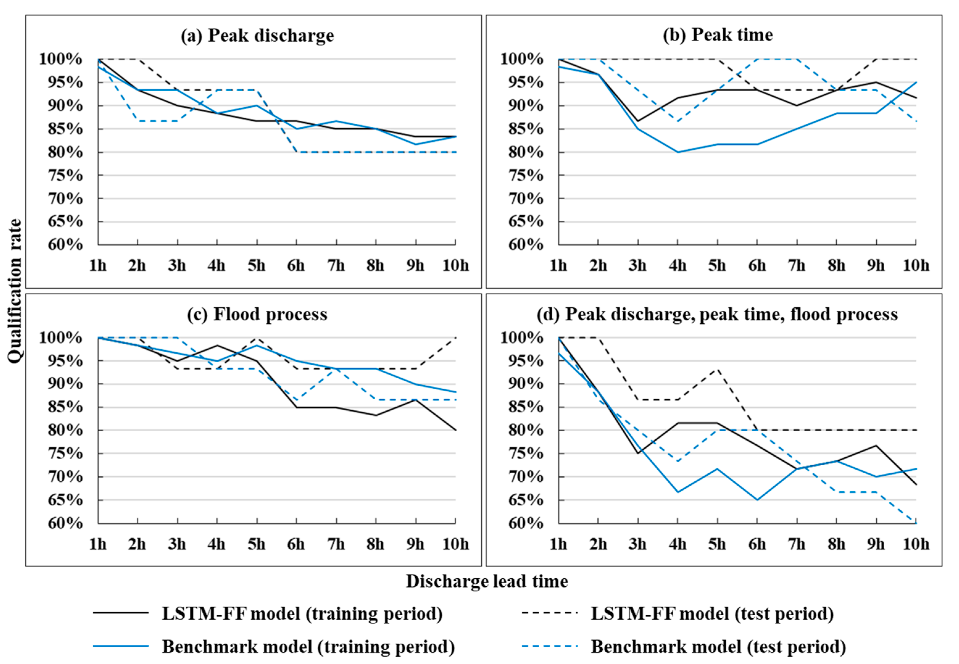
4.1. Model Evaluation

The QR of the training period and test period are compared in Figure 5, in which the solid line represents the training period (training and validation set), and the dashed line represents the test period (test set). As shown in Figure 5a, the QR values of peak discharge in both the training and test period show a decreasing trend with the increase of lead-time and are all above 80.0%. The QR values of the test period are superior to that of the training period until the 5-h lead-time and both of them are above 86.7%. As shown in Figure 5b, the QR values of peak time at the 1–10 h lead-time are relatively stable. The forecasting outcomes at all lead-times during the test period are superior to the results during the training period. Except for the 3 h lead-time of the training period, the QR values are all above 90.0%. The LSTM-FF model outperforms the benchmark model for the test period at the 1–3 h lead-time. Figure 5b shows the lowest QR values of peak time is at the 3 h lead-time. At the 3 h lead-time, all unqualified peak times are from small flood events (27 flood events whose peak discharges are less than 100 m3/s), and most simulated discharge peaks lag 3 h, which is equal to the lead-time of the LSTM network. Thus, we suspect that a relatively small amount of rainfall leads to a major role of the discharge feature and a weaker role of the rainfall feature for small flood events. As shown in Figure 2, at a longer lead-time, the time interval between current time (inputting previous discharge) and forecast time (outputting simulated discharge) is much longer. It limits the role of the discharge feature, so QR values of peak time increase at a 4–10 h lead-time. The LSTM-FF model outperforms the benchmark model for the training period at a 4–9 h lead-time. As shown in Figure 5c, the QR values of the flood process in the training period have a decreasing trend and are all above 80.0%. The QR values of the flood process in the test period keep stable and range from 93.3% to 100%. The LSTM-FF model outperforms the benchmark model for the test period at a 5–10 h lead-time, whereas the training period is the opposite. Figure 5d indicates the QR of all evaluation criteria in the test period are all better than that of the training period. It can be seen from the above analysis that the LSTM-FF model has a good generalization ability (extrapolating ability), and overall outperforms the benchmark model.
The QR values of large flood events (19 flood events whose peak discharge is greater than the threshold discharge) and all 75 flood events for a 1–10 h lead-time are compared in Figure 6. It indicates the QR (peak discharge, peak time, flood process or all of them) of large flood events are superior to that of 75 flood events all at a 1–10 h lead-time, and both show a decreasing trend with the increase of lead-time except peak time. As shown in Figure 6a, the peak discharge QR values of all flood events and large flood events get closer with the increase of lead-time, which is above 82.7%. Specifically, the LSTM-FF model performs exceptionally well at a 1–5 h lead time for the peak discharge QR values of large flood events, which are above 94.7%. In addition, both the peak time and NSE keep high QR, which are above 82.7% and 89.3% at a 1–10 h lead-time in Figure 6b,c. Figure 6a–d illustrates that the LSTM-FF model achieved better-simulated results of peak time and NSE, and simulated peak discharge has a great influence on the overall QR. This confirms that peak discharge is the most critical forecast target in flash flood forecasting. Above all, Figure 6 indicates the LSTM-FF model has more stable and better statistical performances in the simulation of large flood events, which is very crucial for flash flood early warning.
Figure 7 shows the scatter plots of the simulated and observed peak discharge. A few conclusions can be drawn from Figure 7. Firstly, comparing the results of the training, validation, and test set, it shows that the LSTM-FF model has a strong extrapolating ability for large flood events. Secondly, for large flood events, the distribution of scatter plots of a 4–8 h lead-time is close and that of a 9–10 h lead-time is close. It indicates that the RPE of each event changes a little at adjacent lead-times (4–8 h and 9–10 h). The LSTM-FF model explored a similar relation between input and output, although we adopted the strategy of training separately for different lead-times. This will be further confirmed in Section 4.3 later. Thirdly, the LSTM-FF model tends to underestimate the peak discharge (lower than 100 m3/s) in the 4–10 h lead-time.
Figure 8 shows QR of large flood events by different sample sets, in which the red solid line has the same meaning as the one in Figure 6, and the red dash-dotted line represents the simulated results of the small sample set. In this sample set, large flood events are divided into 13 training samples, 3 validation samples, and 3 test samples. Figure 8 indicates no better-simulated results were obtained using only 19 large flood events as the sample set. It is quite different from the LSTM-FF model to the hydrological models. Though the QR in Figure 8 is reduced by small flood events, the contribution of the low discharge process cannot be neglected for the LSTM-FF model. It also suggests that the LSTM-FF model explored the rainfall-runoff relationship from large datasets rather than arbitrary input-output relationships of small datasets.

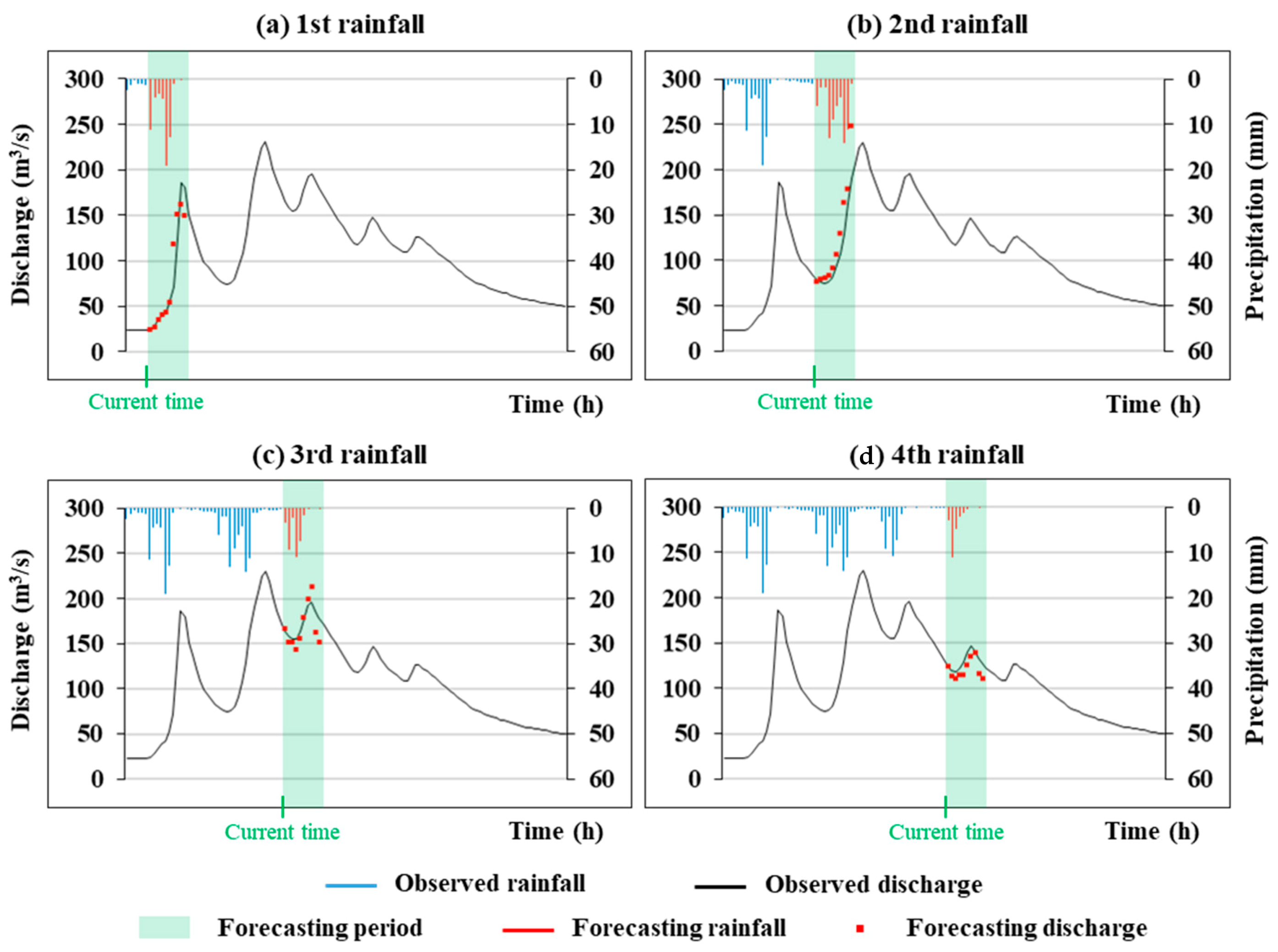
4.2. Model Application

In this section, we choose a multi-peak flood event (20120622) from the test set to show the forecast results as a typical example in discharge real-time forecast. Figure 9 shows the observed and simulated discharge at a 1–10 h lead-time. The black line represents the observed flood hydrograph, and the red dots represent simulated discharges at each lead-time. Obviously, the conclusions drawn in the previous section can be confirmed in Figure 9.
Figure 10 displays the application of the LSTM-FF model at the beginning of four main rainfalls. Four current moments and forecasting periods are marked by green. At each current time, the last 6 h observed rainfall from 8 rainfall stations (part of blue columns), observed discharge (part of black solid line) and the next 10 h short-term precipitation forecast information (red columns) are used to forecast discharges in the 1–10 h lead-time (red dots). Figure 10 indicates that the predicted hydrographs could fit the general trends of the hydrograph well and the LSTM-FF model is a practical tool for discharge forecasting in flash flood prevention.

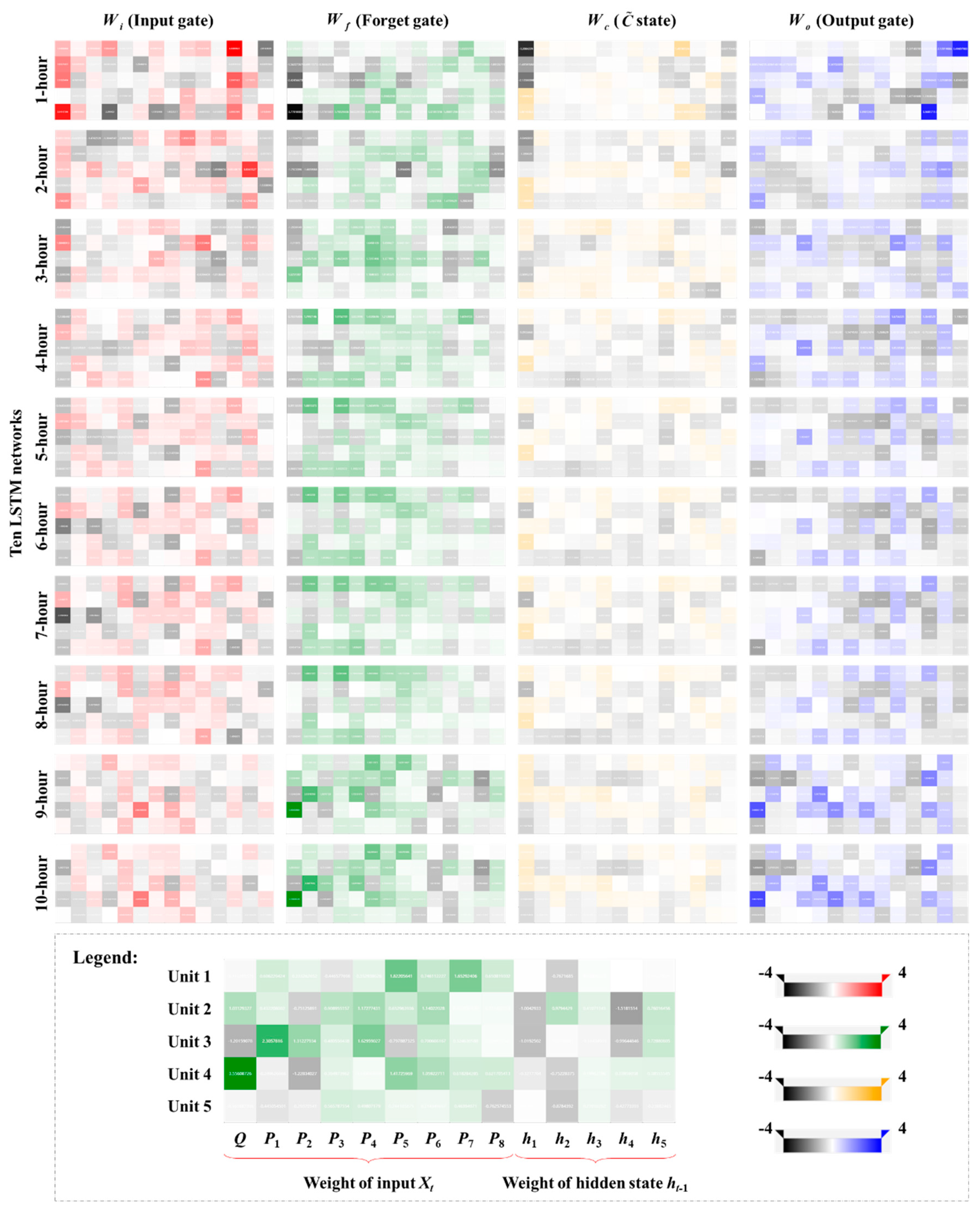
4.3. LSTM Visualization

Ten trained LSTM networks have the same structure with different time steps. If the parameters of these ten LSTM networks are also the same (or similar), it indicates these ten LSTM networks have to find the same (or similar) relationship between input and output. Weight matrices and bias vectors are all parameters in the LSTM-FF model. Therefore, we try to briefly compare and analyze the weight matrices of the input gate, forget gate, candidate state C ˜ t and output gate from ten trained LSTM networks by visualization (see Figure 11). Although it is hard to give a hydrological interpretation of data-driven models, we want to preliminary discuss the effect of the input feature on the weight matrix at different lead times.
As can be seen from Equations (1)–(6) and Section 3, W f ,   W i ,   W c ,   W o are 5 × (9 + 5) matrixes, where the first 5 refers to the dimensions of the input gate, forget gate and candidate state C ˜ t (the number of units), 9 is the number input features (1 discharge and 8 rainfall), and the second five refers to the dimension of h t (the number of units). In every weight matrix of Figure 11, the 1–9 and 10–14 columns represent the weight of input and hidden state, respectively. White indicates the values of weight are close to 0, and the darker the color represents the greater the absolute values of weight. The following conclusions can be drawn: firstly, the first column of the 1 h weight matrix shows a darker color in the input gate, forget gate and candidate state C ˜ t . This phenomenon becomes less obvious as the lead-time increases. It indicates the discharge feature plays a more obvious role in the 1 h LSTM network, and its effect is diminishing with the increase of lead-time. Secondly, the weight matrixes of 4–8 h LSTM networks are alike in each gate, and the 9–10 h LSTM networks also show the same phenomenon. It indicates that in the adjacent lead-time, LSTM networks explored a similar relationship between input and output rather than arbitrary laws. Thirdly, the 10–14 columns of the weight matrix show considerable color variation. It indicates the hidden state also exerts a considerable effect. This is in line with the hydrological process that the discharge of each step is affected by both the previous state (discharge and soil moisture) and the current rainfall.

5. Conclusions

In this paper, the LSTM-FF model, composed of T multivariate single-step LSTM networks, is established to forecast flash floods for a 1−T lead-time. Rainfall distribution, basin time lag, and short-term precipitation forecast are considered in the model structure design. The Anhe catchment located in southeastern China was taken as a case study with qualified rates (QRs) of peak discharge, peak time, and flood process as the evaluation index. The simulated results for different lead-times are analyzed. Moreover, the relationship between simulated results and the weights of the LSTM network are revealed by visualization. The major conclusions can be summarized as follows.
(1)
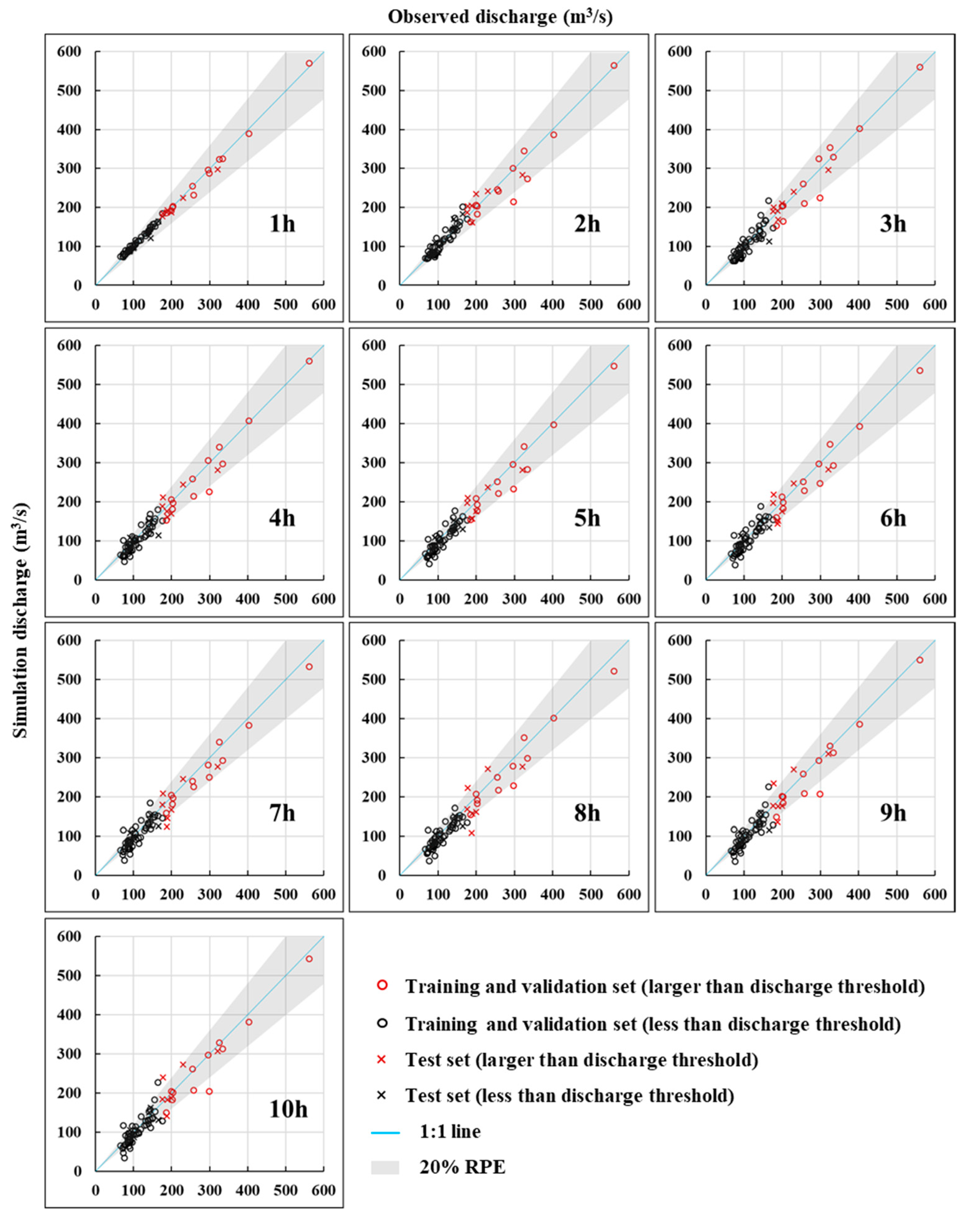
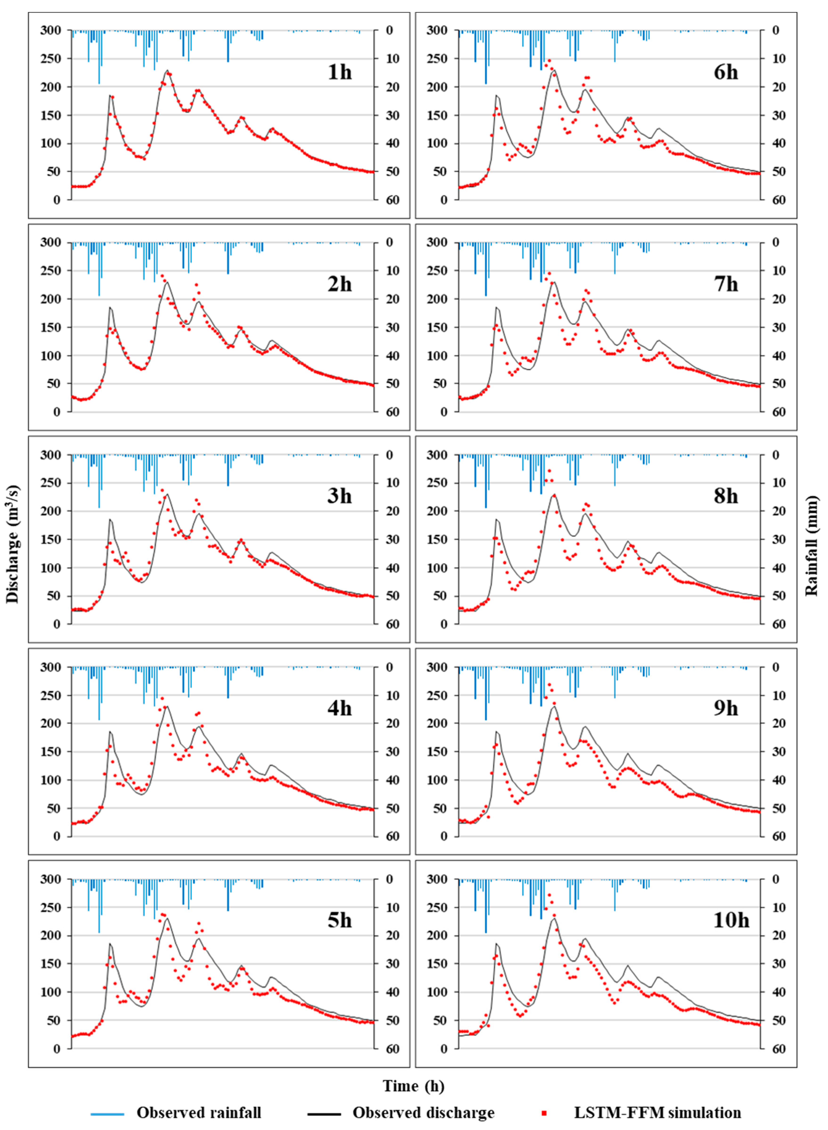
The LSTM-FF model exhibited good performance for flash flood forecasting, and the QR decreases with the increase of lead-time. The QR values of peak discharge, peak time, and flood process are above 82.7%, 89.3%, and 84.0% at a 1–10 h lead time. In addition, the LSTM-FF model has a strong extrapolating ability as the ML model. The LSTM-FF model can be used as a practical tool for flash flood forecasting in mountainous catchments.
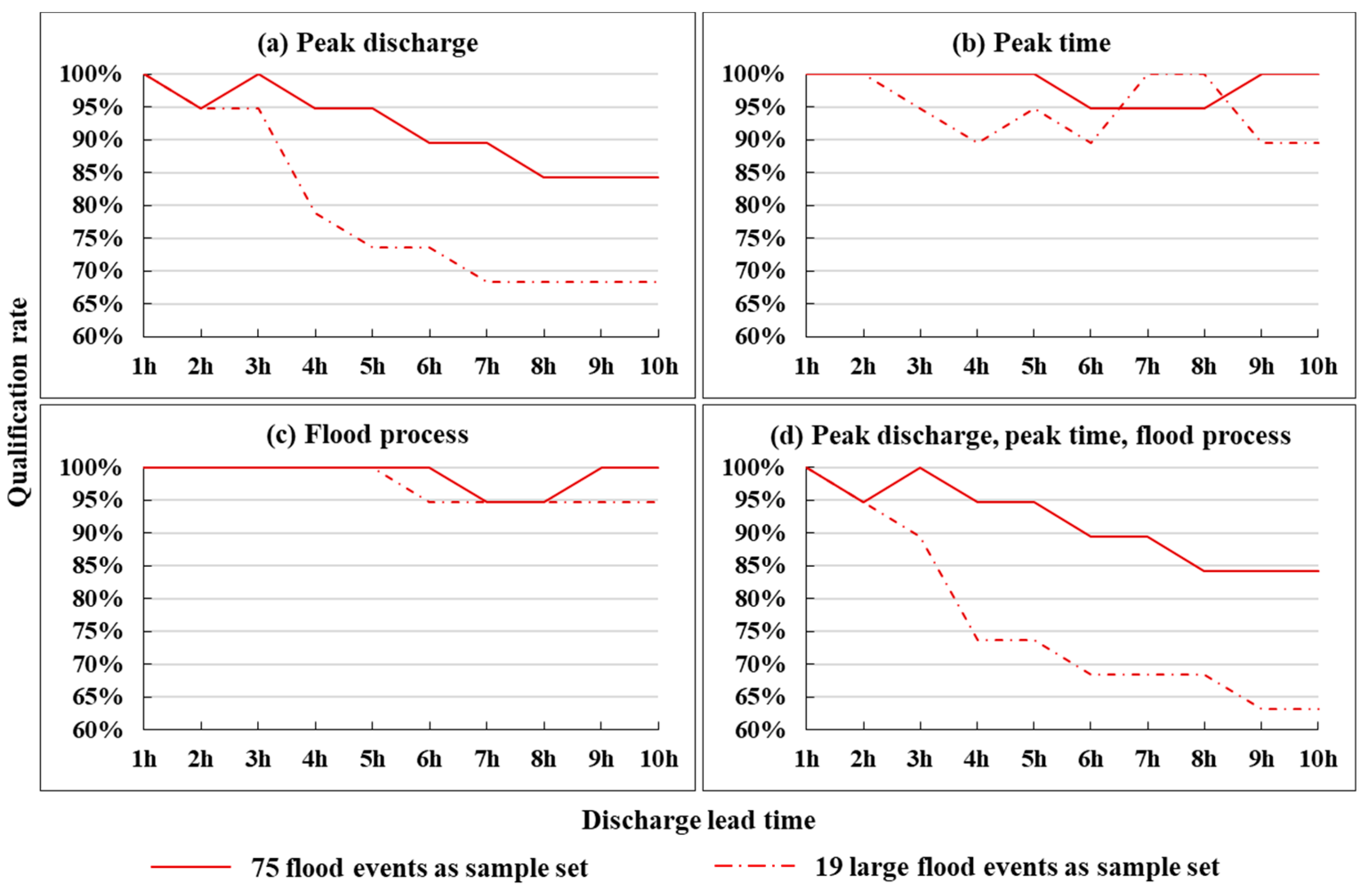
(2)
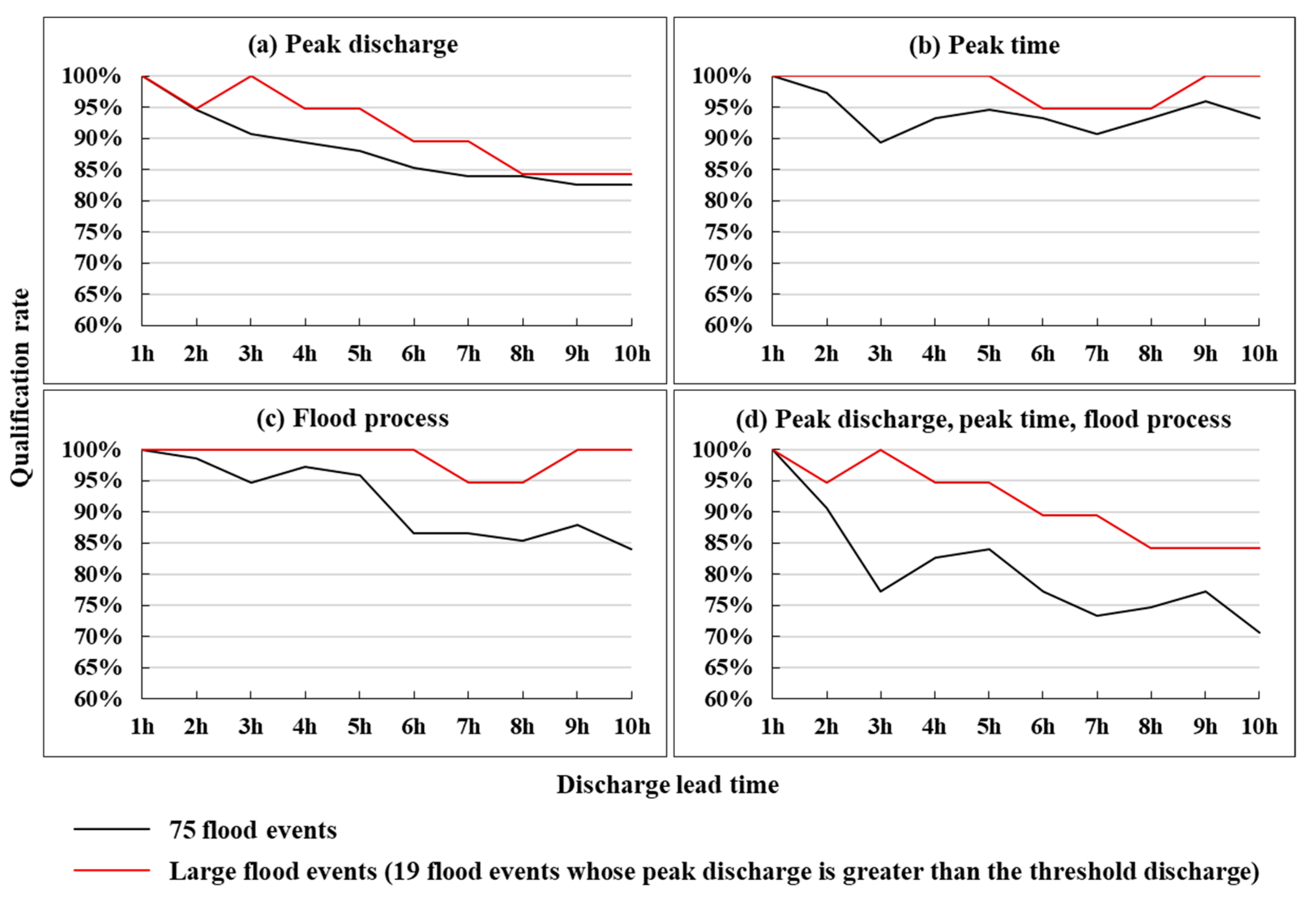
The LSTM-FF model has more stable and better statistical performances in the simulation of large flood events. The QR values of large flood events are above 94.7% at a 1–5 h lead time and range from 84.2% to 89.5% at a 6–10 h lead-time. It is practical and significant for the LSTM-FF model to forecast threshold discharge accurately in flash flood protection.
(3)
Though the QR of small flood events is relatively low, their contribution to training the LSTM-FF model cannot be neglected. No better-simulated results were obtained using only 19 large flood events as a sample set. Flood events with a small discharge-peak can help the LSTM-FF model to explore the rainfall-runoff relationship better.
(4)
The discharge feature plays a more obvious role in the 1 h LSTM network, and its effect is diminishing with the increase of lead-time. In the adjacent lead-time (4–8 h and 9–10 h), LSTM networks explored a similar relationship between input and output.
Further research should focus on the integration of hydrological knowledge and model structure and the interpretation of evolution of LSTM cell state. LSTM networks are also suited for a multivariate multi-step time-series problem and have great potential in the hydrological field. In addition, the influence of rainfall forecast uncertainty on flash flood forecasting results should be further considered.

Author Contributions

T.S. conceptualized, designed the model and wrote the paper. W.D. and H.L. reviewed and edited the paper. H.Z. conceptualized the model. J.W. and J.C. validated the results. All authors have read and agreed to the published version of the manuscript.

Funding

This research was supported by the National Natural Science Foundation of China (Grant No. 2018YFC0407705, 51709036, 91747102, 51879029).

Conflicts of Interest

The authors declare no conflict of interest.

References

  1. Liu, C.; Guo, L.; Ye, L.; Zhang, S.; Zhao, Y.; Song, T. A review of advances in China’s flash flood early-warning system. Nat. Hazards 2018, 92, 619–634. [Google Scholar] [CrossRef] [Green Version]
  2. Douinot, A.; Roux, H.; Garambois, P.A.; Larnier, K.; Labat, D.; Dartus, D. Accounting for rainfall systematic spatial variability in flash flood forecasting. J. Hydrol. 2016, 541, 359–370. [Google Scholar] [CrossRef] [Green Version]
  3. Collier, C.G. Flash flood forecasting: What are the limits of predictability? Q. J. R. Meteorol. Soc. 2010, 133, 3–23. [Google Scholar] [CrossRef]
  4. Hapuarachchi, H.A.P.; Wang, Q.J.; Pagano, T.C. A review of advances in flash flood forecasting. Hydrol. Process. 2011, 25, 2771–2784. [Google Scholar] [CrossRef]
  5. Miao, Q.; Yang, D.; Yang, H.; Li, Z. Establishing a rainfall threshold for flash flood warnings in China’s mountainous areas based on a distributed hydrological model. J. Hydrol. 2016, 541, 371–386. [Google Scholar] [CrossRef]
  6. Reed, S.; Schaake, J.; Zhang, Z. A distributed hydrologic model and threshold frequency-based method for flash flood forecasting at ungauged locations. J. Hydrol. 2007, 337, 402–420. [Google Scholar] [CrossRef]
  7. Blöschl, G.; Reszler, C.; Komma, J. A spatially distributed flash flood forecasting model. Environ. Model. Softw. 2008, 23, 464–478. [Google Scholar] [CrossRef]
  8. Mosavi, A.; Ozturk, P.; Chau, K.W. Flood prediction using machine learning models: Literature review. Water 2018, 10, 1536. [Google Scholar] [CrossRef] [Green Version]
  9. Aichouri, I.; Hani, A.; Bougherira, N.; Djabri, L.; Chaffai, H.; Lallahem, S. River Flow Model Using Artificial Neural Networks. Energy Procedia 2015, 74, 1007–1014. [Google Scholar] [CrossRef] [Green Version]
  10. Talei, A.; Chua, L.H.C. Influence of lag time on event-based rainfall—Runoff modeling using the data driven approach. J. Hydrol. 2012, 438–439, 223–233. [Google Scholar] [CrossRef]
  11. Taormina, R.; Chau, K.W. Data-driven input variable selection for rainfall–runoff modeling using binary-coded particle swarm optimization and Extreme Learning Machines. J. Hydrol. 2015, 529, 1617–1632. [Google Scholar] [CrossRef]
  12. Yaseen, Z.M.; El-Shafie, A.; Jaafar, O.; Afan, H.A.; Sayl, M.N. Artificial intelligence based models for stream-flow forecasting: 2000–2015. J. Hydrol. 2015, 530, 829–844. [Google Scholar] [CrossRef]
  13. Chang, F.J.; Chen, P.A.; Lu, Y.R.; Huang, E.; Chang, K.Y. Real-time multi-step-ahead water level forecasting by recurrent neural networks for urban flood control. J. Hydrol. 2014, 517, 836–846. [Google Scholar] [CrossRef]
  14. Hochreiter, S.; Schmidhuber, J. Long Short-Term Memory. Neural Comput. 1997, 9, 1735–1780. [Google Scholar] [CrossRef] [PubMed]
  15. Kratzert, F.; Klotz, D.; Brenner, C.; Schulz, K.; Herrnegger, M. Rainfall-runoff modelling using Long Short-Term Memory (LSTM) networks. Hydrol. Earth Syst. Sci. 2018, 22, 6005–6022. [Google Scholar] [CrossRef] [Green Version]
  16. Hu, C.; Wu, Q.; Li, H.; Jian, S.; Li, N.; Lou, Z. Deep learning with a long short-term memory networks approach for rainfall-runoff simulation. Water 2018, 10, 1543. [Google Scholar] [CrossRef] [Green Version]
  17. Zhang, D.; Lin, J.; Peng, Q.; Wang, D.; Yang, T.; Sorooshian, S.; Liu, X.; Zhuang, J. Modeling and simulating of reservoir operation using the artificial neural network, support vector regression, deep learning algorithm. J. Hydrol. 2018, 565, 720–736. [Google Scholar] [CrossRef] [Green Version]
  18. Zhang, J.; Zhu, Y.; Zhang, X.; Ye, M.; Yang, J. Developing a Long Short-Term Memory (LSTM) based model for predicting water table depth in agricultural areas. J. Hydrol. 2018, 561, 918–929. [Google Scholar] [CrossRef]
  19. Zhang, D.; Lindholm, G.; Ratnaweera, H. Use Long Short-Term Memory to Enhance Internet of Things for Combined Sewer Overflow Monitoring. J. Hydrol. 2018, 556, 409–418. [Google Scholar] [CrossRef]
  20. Liu, P.; Zhang, X.; Zhao, Y.; Deng, C.; Li, Z.; Xiong, M. Improving efficiencies of flood forecasting during lead times: An operational method and its application in the Baiyunshan Reservoir. Hydrol. Res. 2019, 50, 709–724. [Google Scholar] [CrossRef] [Green Version]
  21. Ntelekos, A.A.; Georgakakos, K.P.; Krajewski, W.F. On the uncertainties of flash flood guidance: Toward probabilistic forecasting of flash floods. J. Hydrometeorol. 2006, 7, 896–915. [Google Scholar] [CrossRef]
  22. Gourley, J.J.; Erlingis, J.M.; Hong, Y.; Wells, E.B. Evaluation of Tools Used for Monitoring and Forecasting Flash Floods in the United States. Weather Forecast. 2012, 27, 158–173. [Google Scholar] [CrossRef] [Green Version]
  23. Carpenter, T.M.; Sperfslage, J.A.; Georgakakos, K.P.; Sweeney, T.; Fread, D.L. National threshold runoff estimation utilizing GIS in support of operational flash flood warning systems. J. Hydrol. 1999, 224, 21–44. [Google Scholar] [CrossRef]
  24. Ripley, B.D. Pattern Recognition and Neural Networks; Cambridge University Press: Oxford, UK, 2007. [Google Scholar]
  25. Liang, C.; Li, H.; Lei, M.; Du, Q. Dongting lake water level forecast and its relationship with the three gorges dam based on a long short-term memory network. Water 2018, 10, 1389. [Google Scholar] [CrossRef] [Green Version]
Figure 1. The internals of a Long Short-Term Memory (LSTM) memory cell.
Water 12 00109 g001
Figure 2. Structure of the LSTM flood forecasting model.
Water 12 00109 g002
Figure 3. Schematic map of Anhe catchment, Henan, China.
Water 12 00109 g003
Figure 4. Partition of the sample set.
Water 12 00109 g004
Figure 5. Qualification rate of the training period and test period.
Water 12 00109 g005
Figure 6. Qualification rate of large flood events and all flood events.
Water 12 00109 g006
Figure 7. Simulated versus observed peak discharge.
Water 12 00109 g007
Figure 8. Qualification rate of large flood events by different sample sets.
Water 12 00109 g008
Figure 9. Observed and simulated discharge of 20120622 flood event.
Water 12 00109 g009
Figure 10. Discharge forecast of 20120622 flood event.
Water 12 00109 g010
Figure 11. Visualization of weight matrices in LSTM networks.
Water 12 00109 g011

