A Regression Model of Stream Water Quality Based on Interactions between Landscape Composition and Riparian Buffer Width in Small Catchments

 , ,
, ,  and
and 
Abstract
:1. Introduction
2. Materials and Methods
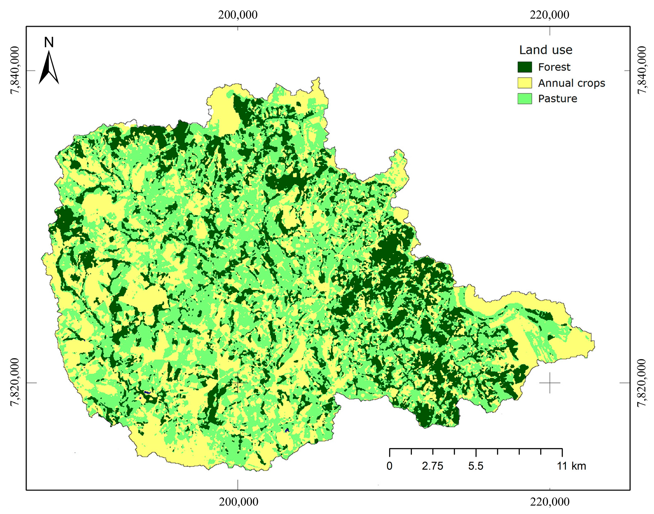
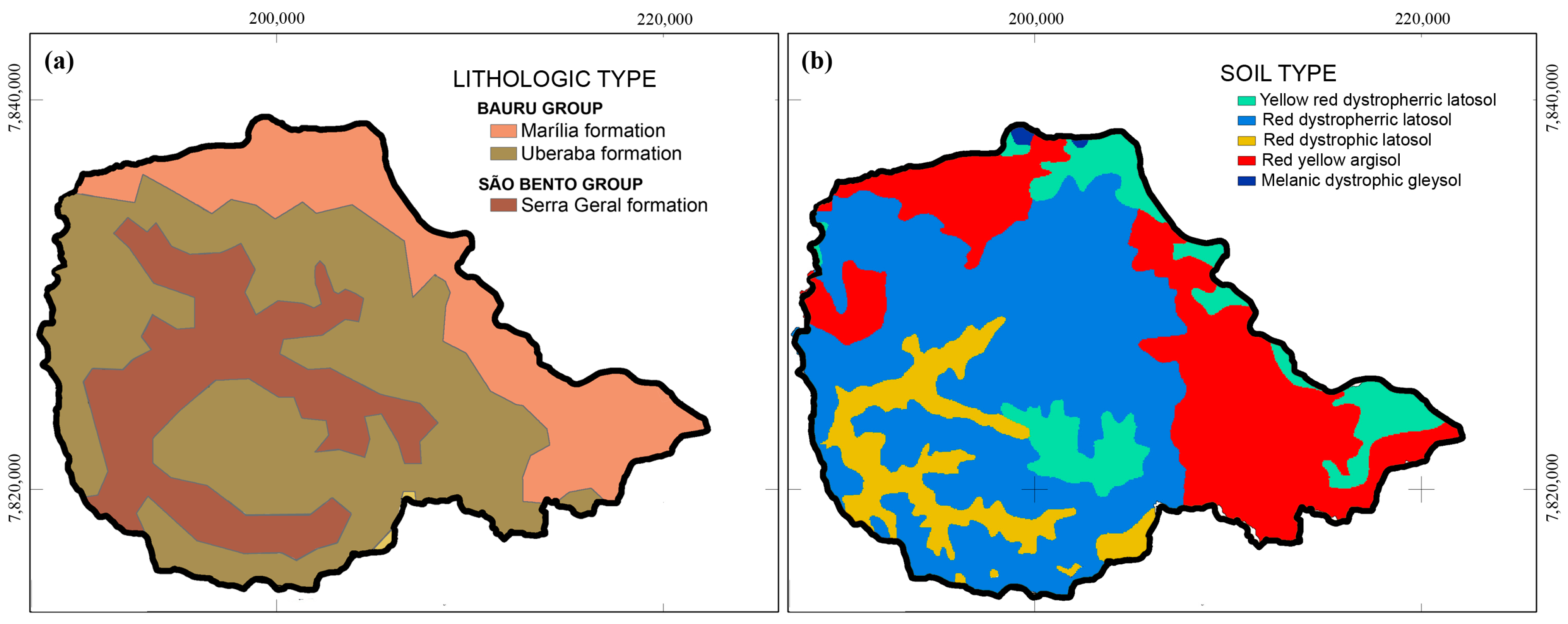
2.1. Study Area
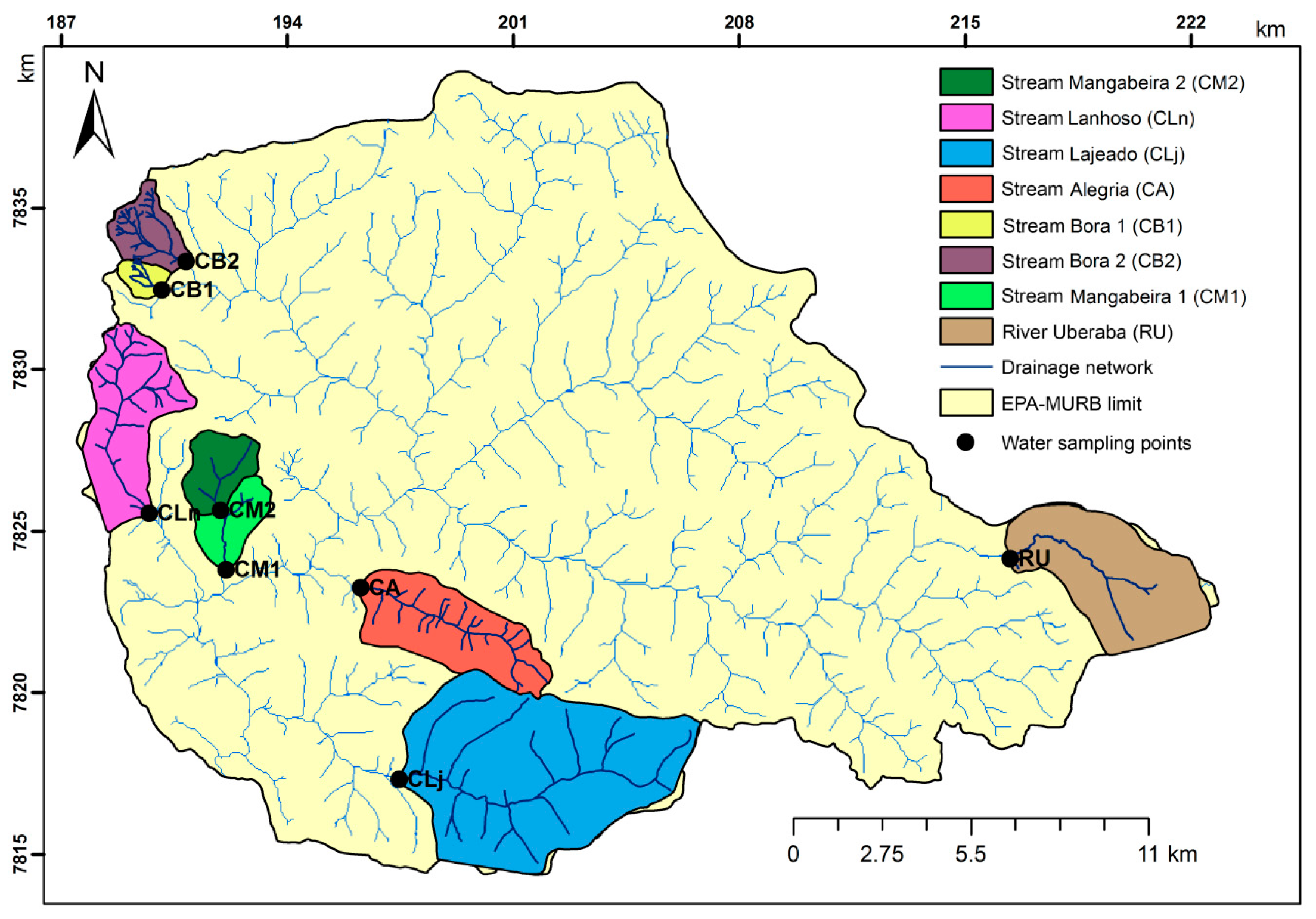
2.2. Studied Sub-Basins
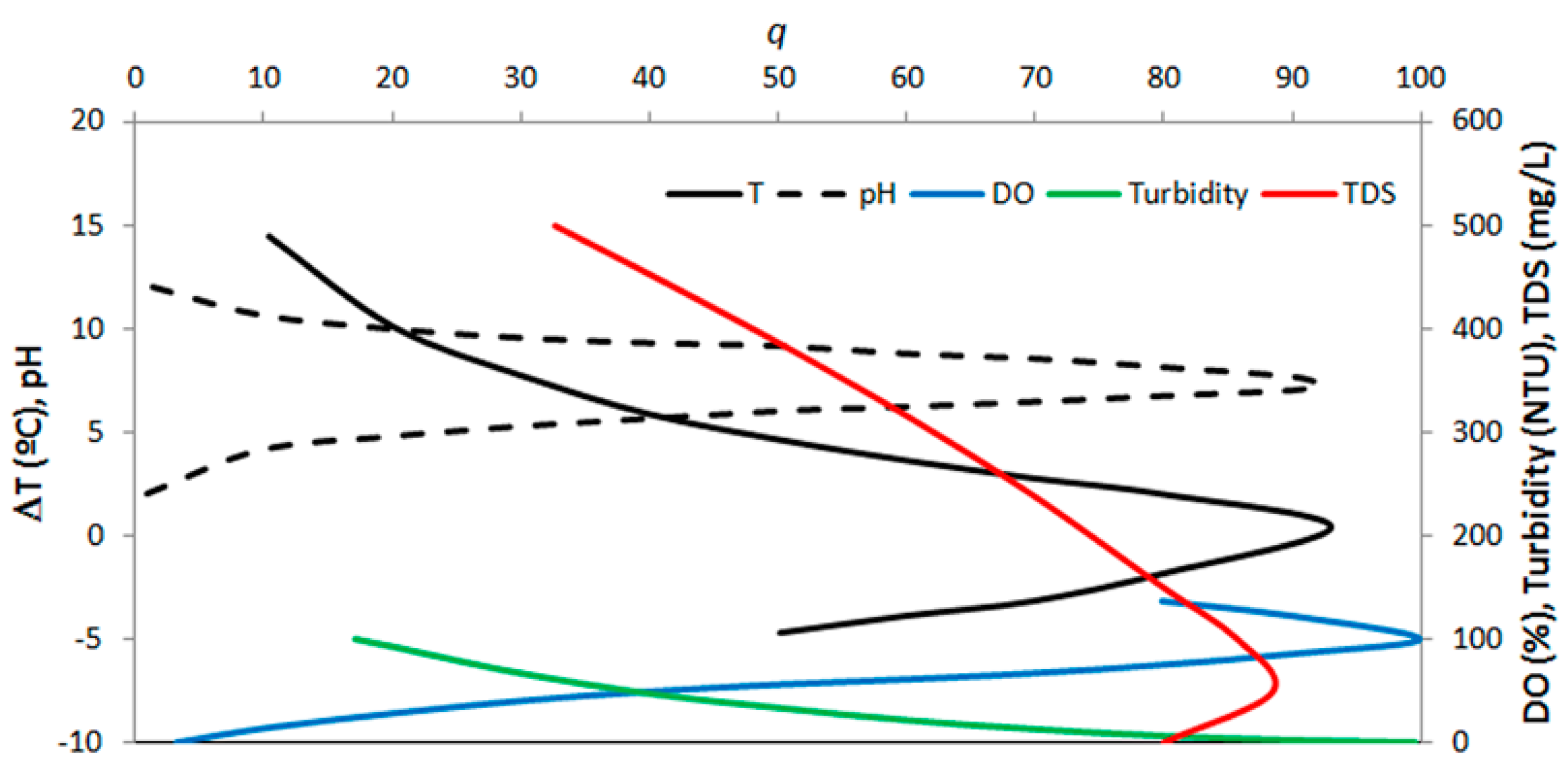
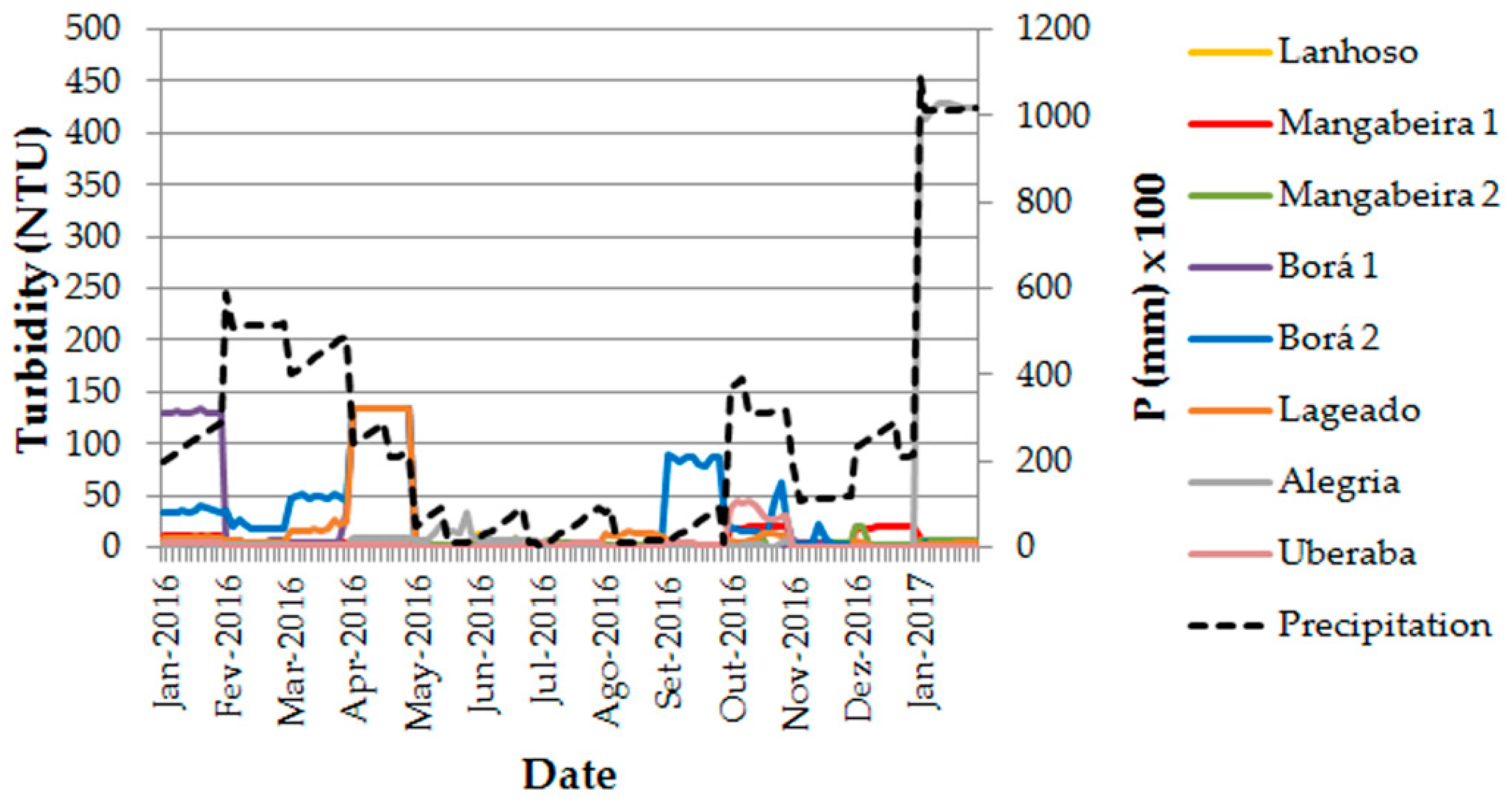
2.3. Water Sampling and Physico-Chemical Analyses
2.4. Multiple Linear Regression with Interactions
2.5. Thematic Maps
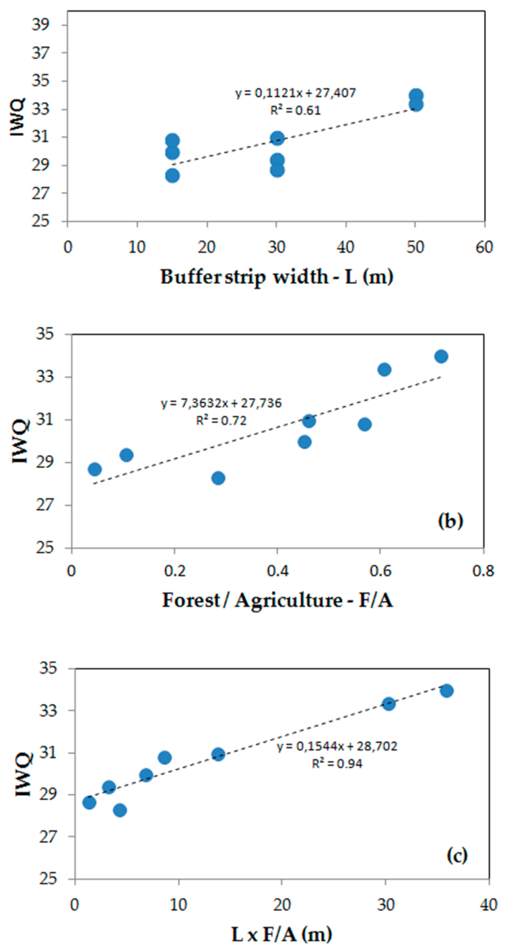
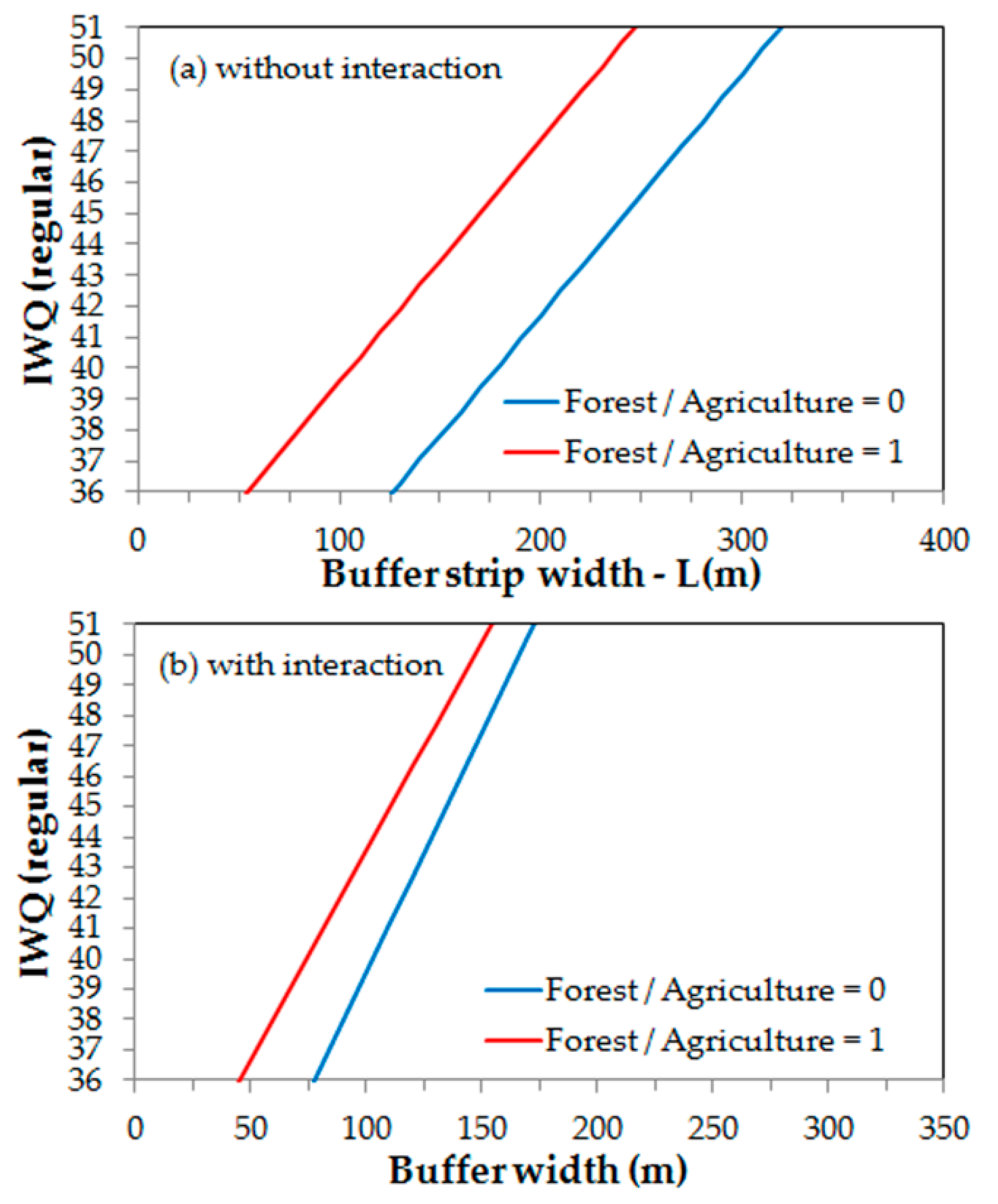
3. Results
4. Discussion
5. Conclusions
Supplementary Materials
Author Contributions
Funding
Acknowledgments
Conflicts of Interest
References
- Cooper, J.R.; Gilliam, J.W. Phosphorus Redistribution from Cultivated Fields into Riparian Areas1. Soil Sci. Soc. Am. J. 1987, 51, 1600–1604. [Google Scholar] [CrossRef]
- Lowrance, R.; Todd, R.; Fail, J.; Hendrickson, O.; Leonard, R.; Asmussen, L. Riparian Forests as Nutrient Filters in Agricultural Watersheds. BioScience 1984, 34, 374–377. [Google Scholar] [CrossRef]
- Peterjohn, W.T.; Correll, D.L. Nutrient Dynamics in an Agricultural Watershed: Observations on the Role of a Riparian Forest. Ecology 1984, 65, 1466–1475. [Google Scholar] [CrossRef]
- Lowrance, R.; Sheridan, J.M. Surface Runoff Water Quality in a Managed Three Zone Riparian Buffer. J. Environ. Qual. 2005, 34, 1851–1859. [Google Scholar] [CrossRef] [PubMed] [Green Version]
- Schoonover, J.E.; Williard, K.W.J.; Zaczek, J.J.; Mangun, J.C.; Carver, A.D. Agricultural Sediment Reduction by Giant Cane and Forest Riparian Buffers. Water Air Soil Pollut. 2006, 169, 303–315. [Google Scholar] [CrossRef]
- Daniels, R.B.; Gilliam, J.W. Sediment and Chemical Load Reduction by Grass and Riparian Filters. Soil Sci. Soc. Am. J. 1996, 60, 246–251. [Google Scholar] [CrossRef]
- Lowrance, R. Groundwater Nitrate and Denitrification in a Coastal Plain Riparian Forest. J. Environ. Qual. 1992, 21, 401–405. [Google Scholar] [CrossRef]
- Hansen, B.D.; Reich, P.; Cavagnaro, T.R.; Lake, P.S. Challenges in applying scientific evidence to width recommendations for riparian management in agricultural Australia. Ecol. Manag. Restor. 2015, 16, 50–57. [Google Scholar] [CrossRef] [Green Version]
- Hill, A.R. Nitrate Removal in Stream Riparian Zones. J. Environ. Qual. 1996, 25, 743–755. [Google Scholar] [CrossRef]
- Hoffmann, C.C.; Kjaergaard, C.; Uusi-Kämppä, J.; Hansen, H.C.B.; Kronvang, B. Phosphorus Retention in Riparian Buffers: Review of Their Efficiency. J. Environ. Qual. 2009, 38, 1942–1955. [Google Scholar] [CrossRef]
- Liu, X.; Zhang, X.; Zhang, M. Major Factors Influencing the Efficacy of Vegetated Buffers on Sediment Trapping: A Review and Analysis. J. Environ. Qual. 2008, 37, 1667–1674. [Google Scholar] [CrossRef]
- Roberts, W.M.; Stutter, M.I.; Haygarth, P.M. Phosphorus Retention and Remobilization in Vegetated Buffer Strips: A Review. J. Environ. Qual. 2012, 41, 389–399. [Google Scholar] [CrossRef] [PubMed]
- Sweeney, B.W.; Newbold, J.D. Streamside Forest Buffer Width Needed to Protect Stream Water Quality, Habitat, and Organisms: A Literature Review. JAWRA J. Am. Water Resour. Assoc. 2014, 50, 560–584. [Google Scholar] [CrossRef]
- Mayer, P.M.; Reynolds, S.K.; Canfiel, T.J. Riparian Buffer Width, Vegetative Cover, and Nitrogen Removal Effectiveness: A Review of Current Science and Regulations; US Environmental Protection Agency: Washington, DC, USA, 2005.
- Valera, C.; Pissarra, T.; Filho, M.; Valle Júnior, R.; Oliveira, C.; Moura, J.; Sanches Fernandes, L.; Pacheco, F. The Buffer Capacity of Riparian Vegetation to Control Water Quality in Anthropogenic Catchments from a Legally Protected Area: A Critical View over the Brazilian New Forest Code. Water 2019, 11, 549. [Google Scholar] [CrossRef]
- Kuehne, R.A. A Classification of Streams, Illustrated by Fish Distribution in an Eastern Kentucky Creek. Ecology 1962, 43, 608–614. [Google Scholar] [CrossRef]
- Uriarte, M.; Yackulic, C.B.; Lim, Y.; Arce-Nazario, J.A. Influence of land use on water quality in a tropical landscape: A multi-scale analysis. Landsc. Ecol. 2011, 26, 1151–1164. [Google Scholar] [CrossRef]
- Beckert, K.A.; Fisher, T.R.; O’Neil, J.M.; Jesien, R.V. Characterization and Comparison of Stream Nutrients, Land Use, and Loading Patterns in Maryland Coastal Bay Watersheds. Water Air Soil Pollut. 2011, 221, 255–273. [Google Scholar] [CrossRef]
- Turner, M.G. Landscape Ecology: The Effect of Pattern on Process. Annu. Rev. Ecol. Syst. 1989, 20, 171–197. [Google Scholar] [CrossRef]
- Townsend, C.R.; Doledec, S.; Norris, R.; Peacock, K.; Arbuckle, C. The influence of scale and geography on relationships between stream community composition and landscape variables: Description and prediction. Freshw. Biol. 2003, 48, 768–785. [Google Scholar] [CrossRef]
- Stryjecki, R.; Zawal, A.; Stępień, E.; Buczyńska, E.; Buczyński, P.; Czachorowski, S.; Szenejko, M.; Śmietana, P. Water mites (Acari, Hydrachnidia) of water bodies of the Krąpiel River valley: Interactions in the spatial arrangement of a river valley. Limnology 2016, 17, 247–261. [Google Scholar] [CrossRef]
- Zhou, T.; Wu, J.; Peng, S. Assessing the effects of landscape pattern on river water quality at multiple scales: A case study of the Dongjiang River watershed, China. Ecol. Indic. 2012, 23, 166–175. [Google Scholar] [CrossRef]
- Tu, J. Spatially varying relationships between land use and water quality across an urbanization gradient explored by geographically weighted regression. Appl. Geogr. 2011, 31, 376–392. [Google Scholar] [CrossRef]
- Rajaei, F.; Sari, A.E.; Salmanmahiny, A.; Delavar, M.; Bavani, A.R.M.; Srinivasan, R. Surface drainage nitrate loading estimate from agriculture fields and its relationship with landscape metrics in Tajan watershed. Paddy Water Environ. 2017, 15, 541–552. [Google Scholar] [CrossRef]
- Teixeira, Z.; Marques, J.C. Relating landscape to stream nitrate-N levels in a coastal eastern-Atlantic watershed (Portugal). Ecol. Indic. 2016, 61, 693–706. [Google Scholar] [CrossRef]
- Awoke, A.; Beyene, A.; Kloos, H.; Goethals, P.L.M.; Triest, L. River Water Pollution Status and Water Policy Scenario in Ethiopia: Raising Awareness for Better Implementation in Developing Countries. Environ. Manag. 2016, 58, 694–706. [Google Scholar] [CrossRef] [PubMed]
- Campagnaro, T.; Frate, L.; Carranza, M.L.; Sitzia, T. Multi-scale analysis of alpine landscapes with different intensities of abandonment reveals similar spatial pattern changes: Implications for habitat conservation. Ecol. Indic. 2017, 74, 147–159. [Google Scholar] [CrossRef]
- Ding, J.; Jiang, Y.; Liu, Q.; Hou, Z.; Liao, J.; Fu, L.; Peng, Q. Influences of the land use pattern on water quality in low-order streams of the Dongjiang River basin, China: A multi-scale analysis. Sci. Total Environ. 2016, 551–552, 205–216. [Google Scholar] [CrossRef]
- Meneses, B.M.; Reis, R.; Vale, M.J.; Saraiva, R. Land use and land cover changes in Zêzere watershed (Portugal)—Water quality implications. Sci. Total Environ. 2015, 527–528, 439–447. [Google Scholar] [CrossRef]
- McMillan, S.K.; Tuttle, A.K.; Jennings, G.D.; Gardner, A. Influence of Restoration Age and Riparian Vegetation on Reach-Scale Nutrient Retention in Restored Urban Streams. JAWRA J. Am. Water Resour. Assoc. 2014, 50, 626–638. [Google Scholar] [CrossRef]
- Goldstein, R.M.; Carlisle, D.M.; Meador, M.R.; Short, T.M. Can Basin Land Use Effects on Physical Characteristics of Streams Be Determined at Broad Geographic Scales? Environ. Monit. Assess. 2007, 130, 495–510. [Google Scholar] [CrossRef]
- Feld, C.K. Response of three lotic assemblages to riparian and catchment-scale land use: Implications for designing catchment monitoring programmes. Freshw. Biol. 2013, 58, 715–729. [Google Scholar] [CrossRef]
- Shen, Z.; Hou, X.; Li, W.; Aini, G. Relating landscape characteristics to non-point source pollution in a typical urbanized watershed in the municipality of Beijing. Landsc. Urban Plan. 2014, 123, 96–107. [Google Scholar] [CrossRef]
- Vikman, A.; Sarkkola, S.; Koivusalo, H.; Sallantaus, T.; Laine, J.; Silvan, N.; Nousiainen, H.; Nieminen, M. Nitrogen retention by peatland buffer areas at six forested catchments in southern and central Finland. Hydrobiologia 2010, 641, 171–183. [Google Scholar] [CrossRef]
- Li, K.; Chi, G.; Wang, L.; Xie, Y.; Wang, X.; Fan, Z. Identifying the critical riparian buffer zone with the strongest linkage between landscape characteristics and surface water quality. Ecol. Indic. 2018, 93, 741–752. [Google Scholar] [CrossRef]
- Shen, Z.; Hou, X.; Li, W.; Aini, G.; Chen, L.; Gong, Y. Impact of landscape pattern at multiple spatial scales on water quality: A case study in a typical urbanised watershed in China. Ecol. Indic. 2015, 48, 417–427. [Google Scholar] [CrossRef]
- Toothaker, L.E.; Aiken, L.S.; West, S.G. Multiple Regression: Testing and Interpreting Interactions. J. Oper. Res. Soc. 1994, 45, 119. [Google Scholar]
- Burks, J.J.; Randolph, D.W.; Seida, J.A. Modeling and interpreting regressions with interactions. J. Account. Lit. 2019, 42, 61–79. [Google Scholar] [CrossRef]
- Kam, C.D.; Franzese, R.J. Modeling and interpreting interactive hypotheses in regression analysis. Choice Rev. Online 2008, 45, 45–3841. [Google Scholar]
- Quintão, D.A.; Caxito, F.D.A.; Karfunkel, J.; Vieira, F.R.; Seer, H.J.; Moraes, L.C.; Ribeiro, L.C.B.; Pedrosa-Soares, A.C. Geochemistry and sedimentary provenance of the Upper Cretaceous Uberaba Formation (Southeastern Triângulo Mineiro, MG, Brazil). Braz. J. Geol. 2017, 47, 159–182. [Google Scholar] [CrossRef]
- Valera, C.A.; Pissarra, T.C.T.; Martins Filho, M.V.; Valle Junior, R.F.; Sanches Fernandes, L.F.; Pacheco, F.A.L. A legal framework with scientific basis for applying the ‘polluter pays principle’ to soil conservation in rural watersheds in Brazil. Land Use Policy 2017, 66, 61–71. [Google Scholar] [CrossRef]
- Valera, C.A.; Valle Junior, R.F.; Varandas, S.G.P.; Sanches Fernandes, L.F.; Pacheco, F.A.L. The role of environmental land use conflicts in soil fertility: A study on the Uberaba River basin, Brazil. Sci. Total Environ. 2016, 562, 463–473. [Google Scholar] [CrossRef] [PubMed]
- Siqueira, H.E.; Pissarra, T.C.T.; do Valle Junior, R.F.; Fernandes, L.F.S.; Pacheco, F.A.L. A multi criteria analog model for assessing the vulnerability of rural catchments to road spills of hazardous substances. Environ. Impact Assess. Rev. 2017, 64, 26–36. [Google Scholar] [CrossRef] [Green Version]
- De Ribeiro, I.V.A.S.; Bouchonneau, N.; Da Silva, A.C.; Fernandes, R.M.C.; De Pinheiro, L.S. Cálculo do índice de qualidade de água (IQA), com estudo de caso nos rios Cocó e Maranguapinho, Ceará. In Proceedings of the Simpósio Brasileiro de Recursos Hídricos, Associação Brasileira de Recursos Hídricos, Campo Grande, Brazil, 22–26 November 2009; p. 18. [Google Scholar]
- ESRI ArcGIS Professional GIS for the Desktop. 2010. Versão 10. Available online: http://desktop.arcgis.com (accessed on 23 August 2019).
- Fonseca, A.R.; Sanches Fernandes, L.F.; Fontainhas-Fernandes, A.; Monteiro, S.M.; Pacheco, F.A.L. The impact of freshwater metal concentrations on the severity of histopathological changes in fish gills: A statistical perspective. Sci. Total Environ. 2017, 599–600, 217–226. [Google Scholar] [CrossRef] [PubMed]
- Fonseca, A.R.; Sanches Fernandes, L.F.; Fontainhas-Fernandes, A.; Monteiro, S.M.; Pacheco, F.A.L. From catchment to fish: Impact of anthropogenic pressures on gill histopathology. Sci. Total Environ. 2016, 550, 972–986. [Google Scholar] [CrossRef] [PubMed]
- Valle Junior, R.F.; Varandas, S.G.P.; Sanches Fernandes, L.F.; Pacheco, F.A.L. Multi Criteria Analysis for the monitoring of aquifer vulnerability: A scientific tool in environmental policy. Environ. Sci. Policy 2015, 48, 250–264. [Google Scholar] [CrossRef] [Green Version]
- Ferreira, A.R.L.; Sanches Fernandes, L.F.; Cortes, R.M.V.; Pacheco, F.A.L. Assessing anthropogenic impacts on riverine ecosystems using nested partial least squares regression. Sci. Total Environ. 2017, 583, 466–477. [Google Scholar] [CrossRef]
- Santos, R.M.B.; Sanches Fernandes, L.F.; Cortes, R.M.V.; Varandas, S.G.P.; Jesus, J.J.B.; Pacheco, F.A.L. Integrative assessment of river damming impacts on aquatic fauna in a Portuguese reservoir. Sci. Total Environ. 2017, 601–602, 1108–1118. [Google Scholar] [CrossRef] [PubMed]
- Sanches Fernandes, L.F.; Fernandes, A.C.P.; Ferreira, A.R.L.; Cortes, R.M.V.; Pacheco, F.A.L. A partial least squares—Path modeling analysis for the understanding of biodiversity loss in rural and urban watersheds in Portugal. Sci. Total Environ. 2018, 626, 1069–1085. [Google Scholar] [CrossRef]
- Álvarez, X.; Valero, E.; Santos, R.M.B.; Varandas, S.G.P.; Sanches Fernandes, L.F.; Pacheco, F.A.L. Anthropogenic nutrients and eutrophication in multiple land use watersheds: Best management practices and policies for the protection of water resources. Land Use Policy 2017, 69, 1–11. [Google Scholar] [CrossRef]
- Pacheco, F.A.L. Regional groundwater flow in hard rocks. Sci. Total Environ. 2015, 506–507, 182–195. [Google Scholar] [CrossRef]
- Fernandes, L.F.S.; Marques, M.J.; Oliveira, P.C.; Moura, J.P. Decision support systems in water resources in the demarcated region of Douro-case study in Pinhão river basin, Portugal. Water Environ. J. 2014, 28, 350–357. [Google Scholar] [CrossRef]
- Fernandes, L.F.S.; dos Santos, C.M.M.; Pereira, A.P.; Moura, J.P. Model of management and decision support systems in the distribution of water for consumption. Eur. J. Environ. Civ. Eng. 2011, 15, 411–426. [Google Scholar] [CrossRef]
- Pacheco, F.A.L.; Van der Weijden, C.H. Weathering of plagioclase across variable flow and solute transport regimes. J. Hydrol. 2012, 420–421, 46–58. [Google Scholar] [CrossRef]
- do Valle Júnior, R.F.; Siqueira, H.E.; Valera, C.A.; Oliveira, C.F.; Sanches Fernandes, L.F.; Moura, J.P.; Pacheco, F.A.L. Diagnosis of degraded pastures using an improved NDVI-based remote sensing approach: An application to the Environmental Protection Area of Uberaba River Basin (Minas Gerais, Brazil). Remote Sens. Appl. Soc. Environ. 2019, 14, 20–33. [Google Scholar] [CrossRef]
- Pacheco, F.A.L.; Szocs, T. “Dedolomitization reactions” driven by anthropogenic activity on loessy sediments, SW Hungary. Appl. Geochem. 2006, 21, 614–631. [Google Scholar] [CrossRef]
- Pacheco, F.A.L. Application of Correspondence Analysis in the Assessment of Groundwater Chemistry. Math. Geol. 1998, 30, 129–161. [Google Scholar] [CrossRef]
- Pacheco, F.A.L.; Landim, P.M.B. Two-Way Regionalized Classification of Multivariate Datasets and its Application to the Assessment of Hydrodynamic Dispersion. Math. Geol. 2005, 37, 393–417. [Google Scholar] [CrossRef] [Green Version]
- Pacheco, F.A.L.; Sousa Oliveira, A.; Van Der Weijden, A.J.; Van Der Weijden, C.H. Weathering, biomass production and groundwater chemistry in an area of dominant anthropogenic influence, the Chaves-Vila Pouca de Aguiar region, north of Portugal. Water Air Soil Pollut. 1999, 115, 481–512. [Google Scholar] [CrossRef]
- Pacheco, F.A.L. Finding the number of natural clusters in groundwater data sets using the concept of equivalence class. Comput. Geosci. 1998, 24, 7–15. [Google Scholar] [CrossRef]
- Hughes, S.J.; Cabecinha, E.; Andrade dos Santos, J.C.; Mendes Andrade, C.M.; Mendes Lopes, D.M.; da Fonseca Trindade, H.M.; dos Santos Cabral, J.A.F.A.; dos Santos, M.G.S.; Lourenço, J.M.M.; Marques Aranha, J.T.; et al. A predictive modelling tool for assessing climate, land use and hydrological change on reservoir physicochemical and biological properties. Area 2012, 44, 432–442. [Google Scholar] [CrossRef]
- Modesto Gonzalez Pereira, M.J.; Sanches Fernandes, L.F.; Barros Macário, E.M.; Gaspar, S.M.; Pinto, J.G. Climate Change Impacts in the Design of Drainage Systems: Case Study of Portugal. J. Irrig. Drain. Eng. 2015, 141, 05014009. [Google Scholar] [CrossRef] [Green Version]
- Miyata, S.; Gomi, T.; Sidle, R.C.; Hiraoka, M.; Onda, Y.; Yamamoto, K.; Nonoda, T. Assessing spatially distributed infiltration capacity to evaluate storm runoff in forested catchments: Implications for hydrological connectivity. Sci. Total Environ. 2019, 669, 148–159. [Google Scholar] [CrossRef] [PubMed]
- Gomi, T.; Sidle, R.C.; Miyata, S.; Kosugi, K.; Onda, Y. Dynamic runoff connectivity of overland flow on steep forested hillslopes: Scale effects and runoff transfer. Water Resour. Res. 2008, 44. [Google Scholar] [CrossRef]
- Gomi, T.; Sidle, R.C.; Ueno, M.; Miyata, S.; Kosugi, K. Characteristics of overland flow generation on steep forested hillslopes of central Japan. J. Hydrol. 2008, 361, 275–290. [Google Scholar] [CrossRef]
- Gomi, T.; Asano, Y.; Uchida, T.; Onda, Y.; Sidle, R.C.; Miyata, S.; Kosugi, K.; Mizugaki, S.; Fukuyama, T.; Fukushima, T. Evaluation of storm runoff pathways in steep nested catchments draining a Japanese cypress forest in central Japan: A geochemical approach. Hydrol. Process. 2010, 24, 550–566. [Google Scholar] [CrossRef]
- Dosskey, M.G.; Helmers, M.J.; Eisenhauer, D.E.; Franti, T.G.; Hoagland, K.D. Assessment of concentrated flow through riparian buffers. J. Soil Water Conserv. 2002, 57, 336–343. [Google Scholar]
- Hénault-Ethier, L.; Larocque, M.; Perron, R.; Wiseman, N.; Labrecque, M. Hydrological heterogeneity in agricultural riparian buffer strips. J. Hydrol. 2017, 546, 276–288. [Google Scholar] [CrossRef]
- Rodrigues, V.; Estrany, J.; Ranzini, M.; de Cicco, V.; Martín-Benito, J.M.T.; Hedo, J.; Lucas-Borja, M.E. Effects of land use and seasonality on stream water quality in a small tropical catchment: The headwater of Córrego Água Limpa, São Paulo (Brazil). Sci. Total Environ. 2018, 622–623, 1553–1561. [Google Scholar] [CrossRef]
- Dai, X.; Zhou, Y.; Ma, W.; Zhou, L. Influence of spatial variation in land-use patterns and topography on water quality of the rivers inflowing to Fuxian Lake, a large deep lake in the plateau of southwestern China. Ecol. Eng. 2017, 99, 417–428. [Google Scholar] [CrossRef]
- Polyakov, V.; Fares, A.; Ryder, M.H. Precision riparian buffers for the control of nonpoint source pollutant loading into surface water: A review. Environ. Rev. 2005, 13, 129–144. [Google Scholar] [CrossRef]
- Damodar Reddy, D.; Subba Rao, A.; Rupa, T.R. Effects of continuous use of cattle manure and fertilizer phosphorus on crop yields and soil organic phosphorus in a Vertisol. Bioresour. Technol. 2000, 75, 113–118. [Google Scholar] [CrossRef]
- Lenka, N.K.; Satapathy, K.K.; Lal, R.; Singh, R.K.; Singh, N.A.K.; Agrawal, P.K.; Choudhury, P.; Rathore, A. Weed strip management for minimizing soil erosion and enhancing productivity in the sloping lands of north-eastern India. Soil Tillage Res. 2017, 170, 104–113. [Google Scholar] [CrossRef] [Green Version]
- Bogunovic, I.; Pereira, P.; Kisic, I.; Sajko, K.; Sraka, M. Tillage management impacts on soil compaction, erosion and crop yield in Stagnosols (Croatia). Catena 2018, 160, 376–384. [Google Scholar] [CrossRef]
- Pacheco, F.A.L.; Varandas, S.G.P.; Sanches Fernandes, L.F.; Valle Junior, R.F. Soil losses in rural watersheds with environmental land use conflicts. Sci. Total Environ. 2014, 485–486, 110–120. [Google Scholar] [CrossRef] [PubMed]
- Shan, N.; Ruan, X.-H.; Xu, J.; Pan, Z.-R. Estimating the optimal width of buffer strip for nonpoint source pollution control in the Three Gorges Reservoir Area, China. Ecol. Modell. 2014, 276, 51–63. [Google Scholar] [CrossRef]
- Bren, L.J. Aspects of the geometry of riparian buffer strips and its significance to forestry operations. For. Ecol. Manag. 1995, 75, 1–10. [Google Scholar] [CrossRef]
- Chang, C.-L.; Hsu, Y.-S.; Lee, B.-J.; Wang, C.-Y.; Weng, L.-J. A cost-benefit analysis for the implementation of riparian buffer strips in the Shihmen reservoir watershed. Int. J. Sediment Res. 2011, 26, 395–401. [Google Scholar] [CrossRef]
- Nigel, R.; Chokmani, K.; Novoa, J.; Rousseau, A.N.; El Alem, A. An extended riparian buffer strip concept for soil conservation and stream protection in an agricultural riverine area of the La Chevrotière River watershed, Québec, Canada, using remote sensing and GIS techniques. Can. Water Resour. J. 2014, 39, 285–301. [Google Scholar] [CrossRef]
- Richit, L.A.; Bonatto, C.; Carlotto, T.; da Silva, R.V.; Grzybowski, J.M.V. Modelling forest regeneration for performance-oriented riparian buffer strips. Ecol. Eng. 2017, 106, 308–322. [Google Scholar] [CrossRef]
- Nigel, R.; Chokmani, K.; Novoa, J.; Rousseau, A.N.; Dufour, P. Recommendations for riparian buffer widths based on field surveys of erosion processes on steep cultivated slopes. Can. Water Resour. J. 2013, 38, 263–279. [Google Scholar] [CrossRef]
- Lin, Y.-F.; Lin, C.-Y.; Chou, W.-C.; Lin, W.-T.; Tsai, J.-S.; Wu, C.-F. Modeling of riparian vegetated buffer strip width and placement. Ecol. Eng. 2004, 23, 327–339. [Google Scholar] [CrossRef]
- Hanowski, J.M.; Walter, P.T.; Niemi, G.J. Effects of prescriptive riparian buffers on landscape characteristics in Northern Minnesota, USA. J. Am. Water Resour. Assoc. 2002, 38, 633–639. [Google Scholar] [CrossRef]


| Sub-Basin | Area (ha) | L (m) | F (%) | A (%) | Other (%) | F/A | L × F/A |
|---|---|---|---|---|---|---|---|
| Alegria | 1263.4 | 15 | 21.3 | 75.4 | 3.3 | 0.3 | 4.2 |
| Lajeado | 3764.8 | 15 | 30.5 | 67.9 | 1.6 | 0.4 | 6.7 |
| Mangabeira 1 | 373.1 | 15 | 36.1 | 63.7 | 0.3 | 0.6 | 8.5 |
| Borá 1 | 136.3 | 30 | 9.3 | 88.8 | 2.0 | 0.1 | 3.1 |
| Mangabeira 2 | 426.6 | 30 | 31.1 | 68.0 | 0.9 | 0.5 | 13.7 |
| Uberaba | 1737.0 | 30 | 3.4 | 81.5 | 15.0 | 0.0 | 1.3 |
| Borá 2 | 409.4 | 50 | 40.5 | 56.7 | 2.8 | 0.7 | 35.7 |
| Lanhoso | 1243.6 | 50 | 37.5 | 62.1 | 0.3 | 0.6 | 30.2 |
| Water Sampling Date | |||||||||||||
|---|---|---|---|---|---|---|---|---|---|---|---|---|---|
| Year | 2016 | 2017 | |||||||||||
| Month | January | February | March | April | May | June | July | August | September | October | November | December | January |
| Day | 19 | 16 | 15 | 19 | 17 | 21 | 19 | 16 | 20 | 18 | 15 | 20 | 17 |
| Rainfall (mm) | |||||||||||||
| Day | 2.0 | 5.9 | 4.0 | 2.4 | 0.5 | 0.2 | 0.0 | 0.8 | 0.1 | 3.7 | 1.9 | 2.3 | 10.9 |
| Day-1 | 8.0 | 8.7 | 5.5 | 1.2 | 2.8 | 0.0 | 0.0 | 0.0 | 0.7 | 4.7 | 13.9 | 2.6 | 27.0 |
| Day-2 | 3.4 | 2.9 | 2.3 | 0.9 | 0.1 | 0.0 | 0.0 | 0.0 | 0.1 | 4.9 | 32.4 | 5.0 | 10.0 |
| Day-3 | 16.6 | 2.8 | 6.3 | 3.7 | 0.9 | 0.0 | 0.0 | 0.0 | 0.0 | 0.6 | 8.4 | 1.4 | 4.4 |
| Sub-Basin | Temperature (°C) | pH | Turbidity (NTU) | DO (%) | TDS (mg/L) | IWQ |
|---|---|---|---|---|---|---|
| Alegria | 20.7 | 7.3 | 35.9 | 80.0 | 0.04 | 28.3 |
| Lajeado | 21.1 | 7.4 | 15.8 | 83.8 | 0.03 | 30.0 |
| Mangabeira 1 | 19.0 | 7.1 | 6.2 | 84.7 | 0.04 | 30.8 |
| Borá 1 | 21.3 | 7.5 | 21.9 | 83.3 | 0.02 | 29.4 |
| Mangabeira 2 | 20.1 | 7.0 | 3.8 | 83.2 | 0.05 | 31.0 |
| Uberaba | 21.1 | 6.2 | 4.3 | 80.8 | 0.03 | 28.7 |
| Borá 2 | 20.3 | 7.5 | 27.3 | 86.7 | 0.05 | 34.0 |
| Lanhoso | 19.7 | 7.4 | 2.0 | 124.8 | 0.06 | 33.4 |
| Term | β | StdError (β) | B | StdError (B) | p-Level |
|---|---|---|---|---|---|
| Without interaction (Adjusted R2 = 0.97) | |||||
| Intercept | 26.14 | 0.32 | 0.0000 | ||
| L | 0.54 | 0.07 | 0.08 | 0.01 | 0.0005 |
| F/A | 0.65 | 0.07 | 5.64 | 0.58 | 0.0002 |
| With interaction (Adjusted R2 = 0.99) | |||||
| Intercept | 23.80 | 0.94 | 0.00 | ||
| L | 1.10 | 0.22 | 0.16 | 0.03 | 0.01 |
| F/A | 1.19 | 0.22 | 10.31 | 1.87 | 0.01 |
| L × F/A | −0.91 | 0.36 | −0.15 | 0.06 | 0.05 |
| Term | b | StdError (b) | B | StdError (B) | p-Level |
|---|---|---|---|---|---|
| Water temperature (Adjusted R2 = 0.10) | |||||
| Intercept | 23.89 | 2.98 | 8.01 | 0.00 | |
| L | −1.69 | −0.09 | 0.10 | −0.92 | 0.41 |
| F/A | −2.10 | −6.94 | 5.93 | −1.17 | 0.31 |
| L × F/A | 2.58 | 0.16 | 0.18 | 0.87 | 0.43 |
| pH (Adjusted R2 = 0.10) | |||||
| Intercept | 8.18 | 1.84 | 4.46 | 0.01 | |
| L | −1.56 | −0.05 | 0.06 | −0.75 | 0.49 |
| F/A | −1.03 | −1.85 | 3.65 | −0.51 | 0.64 |
| L × F/A | 2.58 | 0.09 | 0.11 | 0.77 | 0.48 |
| Turbidity (Adjusted R2 = 0.6) | |||||
| Intercept | 130.65 | 31.49 | 4.15 | 0.01 | |
| L | −4.50 | −3.93 | 1.07 | −3.68 | 0.02 |
| F/A | −4.29 | −225.90 | 62.62 | −3.61 | 0.02 |
| L × F/A | 7.19 | 6.99 | 1.91 | 3.66 | 0.02 |
| Dissolved Oxygen (Adjusted R2 = 0.1) | |||||
| Intercept | 42.48 | 56.08 | 0.76 | 0.49 | |
| L | 1.34 | 1.37 | 1.90 | 0.72 | 0.51 |
| F/A | 0.99 | 60.97 | 111.50 | 0.55 | 0.61 |
| L × F/A | −1.28 | −1.46 | 3.40 | −0.43 | 0.69 |
| Total dissolved solids (Adjusted R2 = 0.45) | |||||
| Intercept | 0.02 | 0.04 | 0.55 | 0.61 | |
| L | 0.10 | 0.00 | 0.00 | 0.07 | 0.95 |
| F/A | 0.67 | 0.04 | 0.08 | 0.48 | 0.65 |
| L × F/A | 0.13 | 0.00 | 0.00 | 0.05 | 0.96 |
© 2019 by the authors. Licensee MDPI, Basel, Switzerland. This article is an open access article distributed under the terms and conditions of the Creative Commons Attribution (CC BY) license (http://creativecommons.org/licenses/by/4.0/).
Share and Cite
Pissarra, T.C.T.; Valera, C.A.; Costa, R.C.A.; Siqueira, H.E.; Martins Filho, M.V.; Valle Júnior, R.F.d.; Sanches Fernandes, L.F.; Pacheco, F.A.L. A Regression Model of Stream Water Quality Based on Interactions between Landscape Composition and Riparian Buffer Width in Small Catchments. Water 2019, 11, 1757. https://doi.org/10.3390/w11091757
Pissarra TCT, Valera CA, Costa RCA, Siqueira HE, Martins Filho MV, Valle Júnior RFd, Sanches Fernandes LF, Pacheco FAL. A Regression Model of Stream Water Quality Based on Interactions between Landscape Composition and Riparian Buffer Width in Small Catchments. Water. 2019; 11(9):1757. https://doi.org/10.3390/w11091757
Chicago/Turabian StylePissarra, Teresa Cristina Tarlé, Carlos Alberto Valera, Renata Cristina Araújo Costa, Hygor Evangelista Siqueira, Marcílio Vieira Martins Filho, Renato Farias do Valle Júnior, Luís Filipe Sanches Fernandes, and Fernando António Leal Pacheco. 2019. "A Regression Model of Stream Water Quality Based on Interactions between Landscape Composition and Riparian Buffer Width in Small Catchments" Water 11, no. 9: 1757. https://doi.org/10.3390/w11091757
APA StylePissarra, T. C. T., Valera, C. A., Costa, R. C. A., Siqueira, H. E., Martins Filho, M. V., Valle Júnior, R. F. d., Sanches Fernandes, L. F., & Pacheco, F. A. L. (2019). A Regression Model of Stream Water Quality Based on Interactions between Landscape Composition and Riparian Buffer Width in Small Catchments. Water, 11(9), 1757. https://doi.org/10.3390/w11091757