1. Introduction
Water distribution networks (WDNs) are critical infrastructure systems that are responsible for securing adequate quantities of safe, high-quality water to the public [
1]. Maintaining a proper functioning of the water systems has always been a primary concern for cities and municipalities because of their direct impact on the health and safety of the people [
2]. Following any hazard, water infrastructures play a dominant role in firefighting and other rescue efforts. Thus, attaining functionality of such critical systems is a more appealing demand after any hazard event [
1]. During their extended service life, WDNs face a broad spectrum of hazards that disturb their functionality and potentially threaten human survival. These hazards that are becoming more frequent and of more damaging consequences are either natural disasters or human-made ones. Earthquakes, floods, hurricanes, extreme temperatures, and climate change are examples of natural hazards that affect the WDNs. Human-made risks may include terrorist attacks, cyber-attacks, overloading, and vandalism [
3]. Aging and deterioration of WDNs increase their vulnerability and the likelihood of function interruption during and after the disruptive events. Pipe breaks, loss of pressure, leaks, and contaminants entering the network are all instances of such consequences [
3]. Traditionally, the focus was placed on physical protection of water systems by avoiding or mitigating the likelihood of disruptive events and their adverse impacts [
4]. However, because of the high uncertainty nature of hazards and complex interdependency of infrastructure systems, it is not possible to protect water networks from all hazards using classical strategies. Therefore, infrastructure resilience is emerging as an essential consideration in the planning and management of WDNs. In this context, water networks will be strong enough to withstand any disruption with a minimum impact on its performance and to recover quickly in case of service loss [
4]. Resilience capabilities in infrastructure systems are usually described by three main aspects, namely: absorptive, adaptive, and restorative capacities [
5]. Absorptive capacity measures the ability of a system to withstand the impact of a hazard event with minimum disruption in the services it provides. Adaptive capacity measures the system’s capability to adjust itself under a new disrupted state and to continue delivering its service. Restorative capacity is a measure of the system’s ability to recover efficiently. The American Society of Civil Engineers defines resilience of infrastructure systems as the ability to mitigate all-hazard risks and rapidly recover critical services with minimum harm to the public safety, health, economy, and national security [
6]. This definition, among others reported in the literature, interprets resilience of infrastructure systems as a process that inherits the four distinct phases. The process always starts with some preparedness measures to mitigate the impacts of anticipated hazards. After the occurrence of a hazard event, a response process starts, and recovery actions are taken to restore the service. Subsequently, policies are revised to be better prepared for the next hazard events.
The literature includes various models and frameworks that evaluate the resilience of water systems and WDNs. Approaches in this area can be broadly classified into two main categories: qualitative approaches and quantitative approaches [
2]. Qualitative approaches can be either in the form of conceptual frameworks or as semi-quantitative indices [
7]. Fisher et al. [
8] developed an index to measure the resilience of critical infrastructures, including water systems. The model involved extensive data collection of about 1500 variables categorized under robustness, recovery, and resourcefulness. The variables were then weighted and summed to generate a single global resilience index that allows the comparison between different infrastructure systems [
8]. Fiksel et al. [
9] developed another example of conceptual frameworks to evaluate the resilience of water systems by assessing several factors such as vulnerability, recoverability, resource productivity, cohesion, adaption, and diversity. Such approaches are usually subjective, and the results cannot be generalized on a large scale of water systems. Quantitative approaches for measuring resilience may also be classified as either probabilistic or deterministic depending on whether the stochastic nature of the system functions is considered. Each approach can be further clustered as a dynamic approach or a static one. The former considers the time-dependent functions of a system, while unlike the latter [
2]. Todini [
10] introduced a resilience metric as a measurement of the excess power in a system and demonstrated its applicability in the design of WDNs. Jayaram and Srinivasan [
11] extended Todini’s metric to account for multiple sources in network resilience quantification. In their research study, the authors obtained a trade-off between life-cycle cost and modified resilience index using multi-objective optimization. The life cycle cost comprised of installation cost, replacement cost, cleaning and lining cost, breakage cost, and salvage value. The authors simulated a sample network over an extended period while increasing the roughness of water pipes to capture the hydraulic deterioration of the network. The authors reported considerable cost savings by considering the design and rehabilitation together instead of exclusively focusing on overdesigning the network. Suribabu [
12] utilized the previous two metrics to optimize the design of WDNs. In his work, he considered minimizing the cost of network resilience enhancement subject to specific pipe diameters and pressure head constraints. The optimization model suggested configuring the network such that the pipe sizes are decreasing along the shortest path. In a different research study to optimize the design of WDN, Choi and Kim [
13] formulated a multi-objective model that considers mechanical redundancy under multiple pipe failures of different states. The study derived a relationship between pipe failure states and mechanical redundancy. Also, the authors analyzed, through simulation, the demand levels of abnormal situations based on extreme demands. In that study, system hydraulic ability was used as an indication of the system’s redundancy; however, other redundancy measures of topological characteristics can be used. Another extension of the resilience index proposed by Todini can be found in a study presented by Creaco et al. [
14]. In his study, Creaco et al. [
14] extended the original resilience index by using pressure-driven modeling and accounting for the energy dissipated by leaks through the water pipes. The authors studied time variation of resilience resulting from changing pipe leakage and roughness coefficients while investigating the cost of the network. The reported cost and delivered power of the configuration obtained after these modifications outperformed the corresponding values obtained by the original index suggested by Toodini [
10].
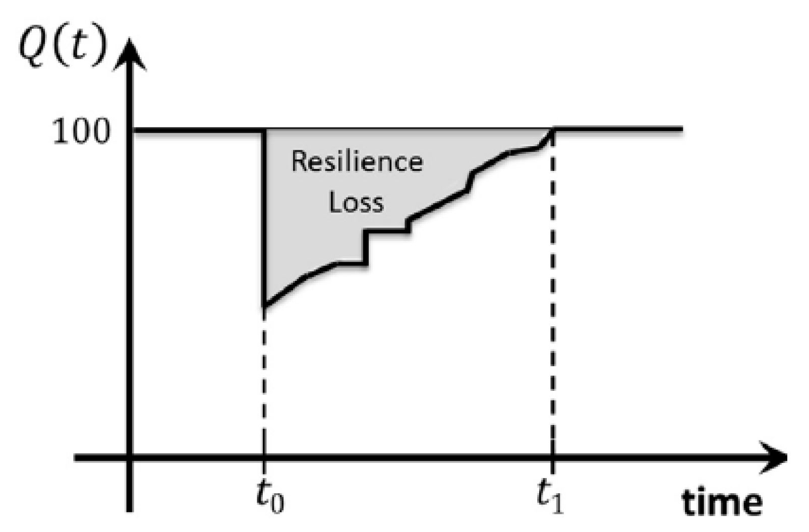
Bruneau et al. [
15] developed one of the most widely used metrics for resilience assessment. In their work, the authors calculated the resilience loss,
RL, as a deterministic dynamic metric that captures the degradation of a system following a hazard event, Equation (1).
where
is the resilience loss,
is a quality function that measures the system performance as a percentage,
is the time at which the disruption occurs, and
t1 is the time at which the resilience is calculated.
can be any performance indicator of the system. In this method, the initial performance of the system is assumed to be 100, and the shaded area represents the resilience loss, as shown in
Figure 1 [
15,
16,
17]. An extension of this method is found in the research effort done by Henry and Ramirez-Marquez [
18]. The authors defined three distinct states, namely: original stable (
S0), disrupted (
Sd), and stable recovered (
Sf) that depict the states of any system before, during, and after the occurrence of a hazard, respectively. Equation (2) is used to calculate the resilience as a ratio between the recovery level at any instant to the initial loss in the performance function [
18,
19,
20,
21].
where
ЯF(
|
) is the proportion of delivery function that has been recovered from the disrupted state under event
,
is the figure-of-merit of the system at the recovered state
,
is the figure-of-merit of the system at the disrupted state
under the event
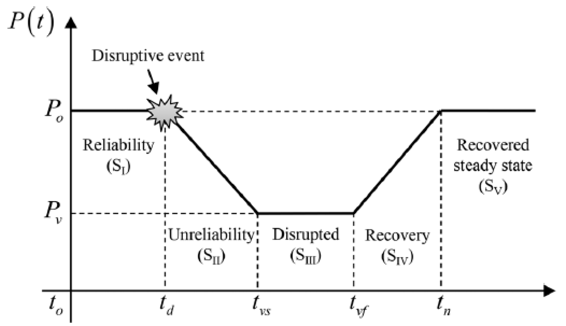
. Dessavre et al. [
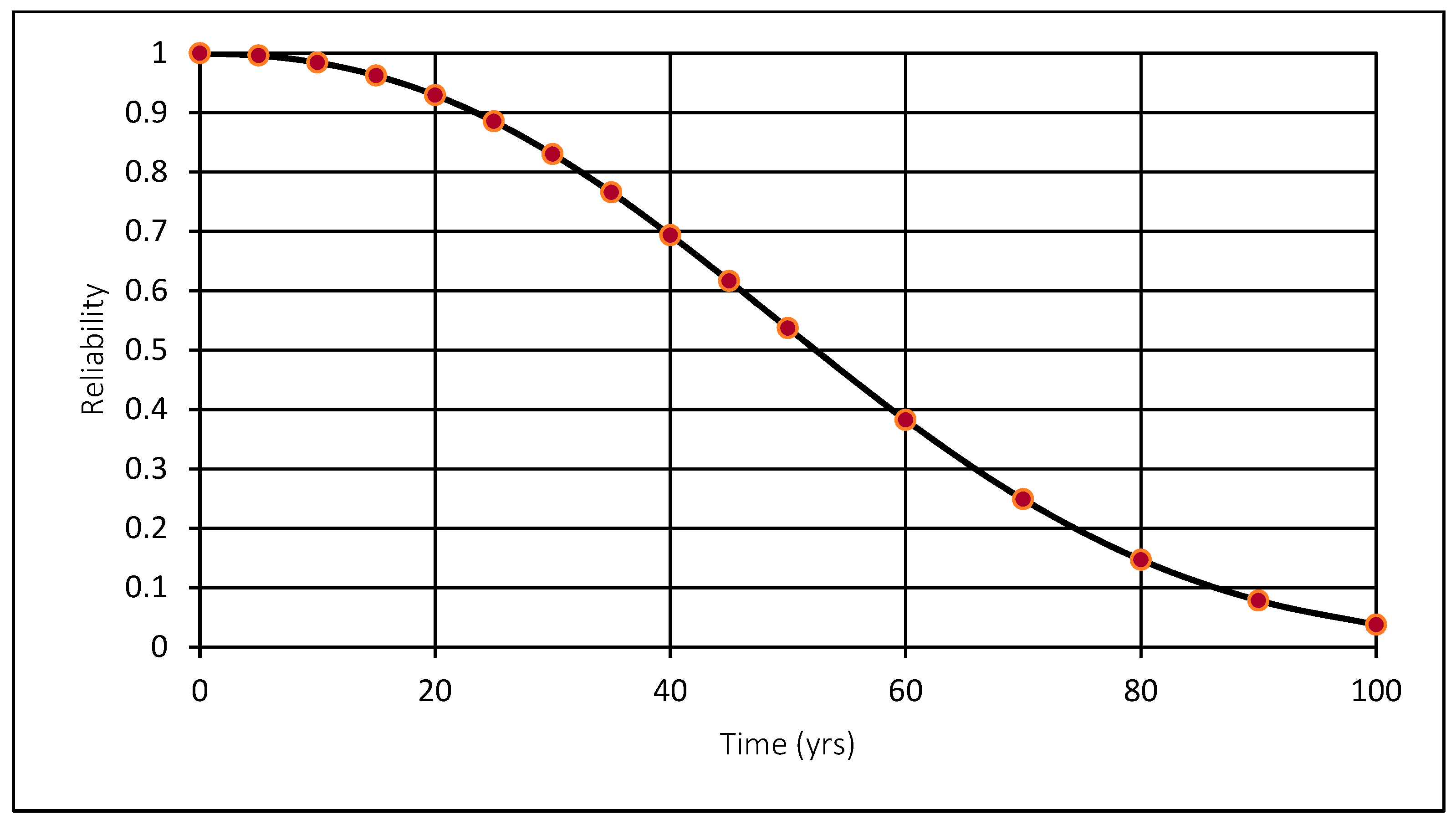
21] formulated a five-states resilience framework for assessing the resilience of urban infrastructure systems before, during, and after the disruption events.
Figure 2 illustrates their model, starting from a steady reliability state when a system functions normally before the occurrence of a disruptive event. At that instant, the system undergoes a transition state beginning with a gradual reduction in its performance, followed by an idle period for damage estimation and restoration planning. This transition finally ends by a course of recovery actions to restore service provision. The final recovered steady state may be either same, less, or even more than the initial state before the disruption occurrence [
21].
Ouyang et al. [
22] extended previous approaches to present a stochastic time-dependent metric for measuring the annual resilience against multi-hazard events. This metric, given in Equation (3), measures resilience as the mean ration between the actual performance curve,
, and the target performance curve,
, over a time period (
) which equals one year in the original model.
where
is the annual resilience and
is the mean operator. Zhao et al. [
23] employed this time-based resilience measure to compare the technical and organizational effects of two post-disaster rebuilding strategies: pipeline ductile retrofitting and network meshed expansion. They concluded that retrofitting is a preferred strategy to enhance seismic resilience of WDNs under limited recovery budget and resources, whereas meshed expansion can increase the performance of WDNs in the case of sufficient fund availability. Several previous studies followed an approach of depicting resilience as the antonym of system vulnerability [
24,
25]. For example, Baroud et al. [
24] developed a model to assess the resilience based on vulnerability and recoverability of waterway networks. The authors employed two stochastic measures to rank the links in a network based on their importance. A multicriteria comparison technique was utilized to produce the order of the ranked components. Other authors compared the resilience index and the entropy index in rehabilitation planning of WDNs. For example, Cimorelli et al. [
26] suggested a rehabilitation methodology to increase two surrogate reliability measures subject to a limited budget. They compared the performance of the resilience index suggested by Creaco et al. [
14] and entropy index based on two case studies. The authors found that the considered resilience index is more accurate in reliability estimations. It was also recommended to consider demand satisfaction when using the entropy index in constrained budget rehabilitation of WDNs. In some studies, indicators from graph theory were employed, such as connectivity, link density, meshed-ness, spectral gap, and central-point dominance to provide quick and practical resilience indicators [
27,
28,
29]. Some authors focused their studies on the loss estimation and restoration efforts in the context of seismic resilience [
30,
31]. Farahmandfar et al. [
31] compared the performance of topology-based and flow-based metrics in optimizing the selection of rehabilitation strategies of large WDNs which are prone to seismic hazards. The decision variables included a combination of pipeline replacements and new pipeline installations. The objective was to achieve the maximum enhancement of resilience given a capital budget constraint. The results indicate that the flow-based metric is relativity more accurate; however, it is suffering from significant computational time.
Consulting the literature about resilience assessment of WDNs reveals several remarks. Generally, more efforts focused on incorporating resilience in the design phase of WDNs compared to incorporating resilience during the operation and maintenance of WDNs. Most of these models depend mainly on running complex hydraulic simulations. The main issue with hydraulic simulation-based methods is that they require complicated calculations and parameters calibration, which significantly increase the computational cost, especially as the size and complexity of the network increase [
32]. Many researchers have tackled resilience from a disaster management perspective, “a snapshot in time” disregarding some important asset management concepts such as deterioration and aging of water networks [
33]. Research efforts that investigated such concepts usually tend to assume the expected level of deterioration. For example, both Jayaram and Srinivasan [
11] and Creaco et al. [
14] investigated the effects of deterioration through hydraulic simulation by increasing the roughness of water pipes. However, the rates of roughness growth were assumed in both studies. There is still a need to adopt more accurate methods in estimating the deterioration of WDNs. This will facilitate investigating a long-term variation of resilience during the operation phase, which will help guide the investments in WDNs and preparedness plans.
On the other hand, approaches based on graph theory rarely consider other non-topological characteristics of WDNs such as pipe lengths, diameters, aging effects, and previous failure history. Including such factors yields better estimates of resilience levels of the WDNs, which will help in deriving optimum enhancement and restoration plans. Additionally, most of the previous research studies that investigated the probability of failure were limited to analyzing one specific source of hazard, such as earthquakes. There is a need to shift the emphasis to analyze the impact of risks on the network, which will facilitate addressing several hazards that result in the same impacts in one single analysis. Furthermore, few efforts have considered various dimensions of resilience in a single metric that can be readily used in real-world applications. For example, some components might be of a higher economic and social criticality (e.g., pipe segments delivering water to hospitals) and require a more rapid recovery than other components.
The objective of this paper is to present a newly developed metric for assessing resilience of WDNs that overcomes the previous limitations, and to demonstrate its applicability in selecting efficient enhancement and recovery strategies. The rest of this paper is organized as follows: In
Section 2, the multi-attribute resilience metric is introduced where the underlying concepts and mathematical formulation are presented in detail. In
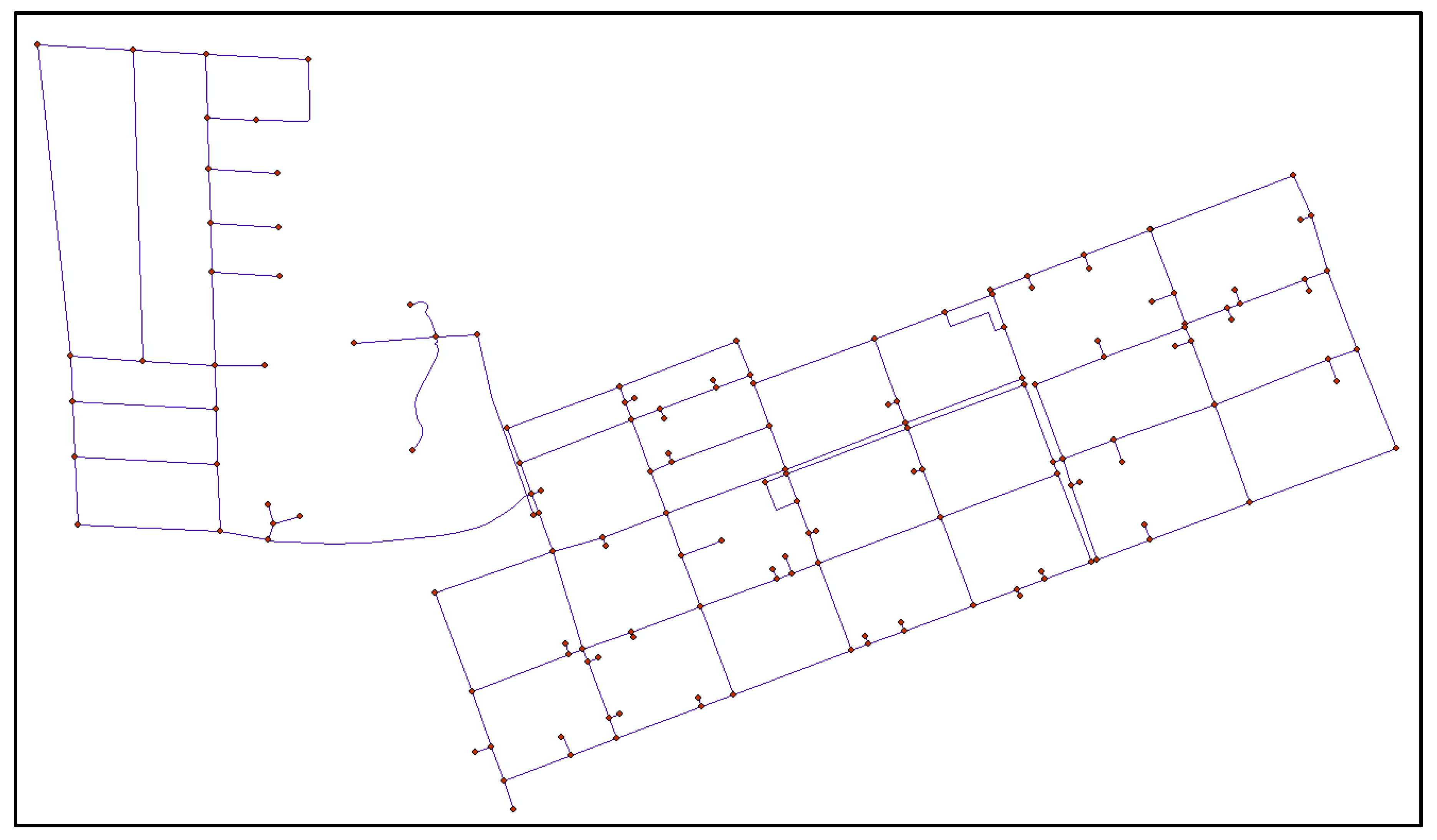
Section 3, the developed metric is used to evaluate the resilience of an actual WDN in the City of London, Ontario. An optimization framework is then presented to select the optimal resilience enhancement plan. This section also includes a hypothetical example to illustrate the practicality of using the proposed resilience metric in selecting the best restoration strategy. The computed resilience levels are then compared to values obtained by previously developed metrics. Conclusions are drawn in
Section 4 along with the research limitations and recommendations for future studies.


