Article

Sea Surface Circulation Structures in the Malta-Sicily Channel from Remote Sensing Data

by
Nydia C. Reyes Suarez
1,2,*,
Michael S. Cook
3,
Miroslav Gačić
2,
Jeffrey D. Paduan
3,
Aldo Drago
4 and
Vanessa Cardin
1
1
Istituto Nazionale di Oceanografia e di Geofisica Sperimentale—OGS, 34010 Sgonico (TS), Italy
2
TRIL Programme, Abdus Salam International Center for Theoretical Physics—ICTP, 34151 Trieste, Italy
3
Department of Oceanography, Naval Postgraduate School—NPS, Monterey, CA 93943, USA
4
Physical Oceanography Research Group, Department of Geosciences, University of Malta, 2080 Msida, Malta
*
Author to whom correspondence should be addressed.
Water 2019, 11(8), 1589; https://doi.org/10.3390/w11081589
Submission received: 20 June 2019 / Revised: 17 July 2019 / Accepted: 25 July 2019 / Published: 31 July 2019
(This article belongs to the Special Issue Ocean Exchange and Circulation)

Abstract

:
The Malta-Sicily Channel is part of the Sicily Channel system where water and thermohaline properties between the Eastern and Western Mediterranean basins take place. Several mesoscales features are detached from the main circulation due to wind and bathymetric forcing. In this paper, surface circulation structures are studied using different remotely sensed datasets: satellite data (absolute dynamic topography, Cross-Calibrated Multi-Platform wind vector analysis, satellite chlorophyll and sea surface temperature) and high frequency radar data. We identified high frequency motions (at short time scales—hours to days), as well as mesoscale structures fundamental for the understanding of the Malta-Sicily Channel circulation dynamics. One of those is the Malta-Sicily Gyre; an anticyclonic structure trapped between the Sicilian and Maltese coasts, which is poorly studied in the literature and often confused with the Malta Channel Crest and the Ionian Shelf Break Vortex. In order to characterize this gyre, we calculated its kinetic properties taking advantage of the fine-scale temporal and spatial resolution of the high frequency radar data, and thus confirming its presence with an updated version of the surface circulation patterns in the area.

1. Introduction

Study Area

Although smaller than the synoptic scale, mesoscale to sub-mesoscale structures influence the stratification and contribute to the vertical and horizontal advection of sea water properties. Due to the small Rossby radius of deformation in the Mediterranean Sea (15–20 km) the typical mesoscale features are characterized by scales of the order of 10–100 km [1,2]. The circulation in the Sicily Channel (SC; defined as 11–16.5° E and 33—38° N in Figure 1 for our studies) is mainly driven by the Mediterranean thermohaline circulation together with its mesoscale and seasonal variability showing intra-annual and inter-annual variability [3,4,5]. This area is characterized by a complex bathymetry with a two-sill system at the Sicily Strait (SS) [6]. On the Italian side, the sill is very narrow with a maximum depth of ~430 m, while on the Tunisian side it is wider and shallower with a sill depth of ~360 m [7]. The exit to the Ionian Sea is bounded by the Malta Plateau and the Medina Bank (MP and MB in Figure 1). In the center of the SC three important depressions are present; the Pantelleria trough (PT; ~1300 m depth), the Linosa trough (LT; ~1500 m depth) and the Malta trough (MT; ~1700 m depth). These bathymetric features can strongly influence the current system in the SC.
Contrary to the SC, the Malta-Sicily Channel (hereafter referred as the channel) is a shelf in the mid Mediterranean Sea that separates the Malta island from the southern tip of Sicily. Topographically this shelf is characterized by a plateau in the middle (MP) with an average depth of 150 m as shown in Figure 1. On its northwestern side the shelf is bounded by the submarine ridges aforementioned with depressions reaching 1700 m deep where the Maltese islands represent the emerged part of the ridge [8]. On its southeastern side, the channel abruptly deepens into the Ionian Sea (~3000 m deep) due to the presence of the Sicily-Malta Escarpment (~2500 m deep) which is one of the largest and least explored underwater cliffs in the Mediterranean Sea [8]. The circulation on longer time scales (lower frequency) is mainly driven by the Atlantic Ionian Stream (AIS) and the Malta-Sicily Gyre (MSG), where the latter has been identified as a quasi-permanent structure with highest incidence in the winter period and related to the variability of the AIS [9,10]. In addition, the Malta-Sicily Gyre (MSG) has been poorly described in the literature, and is often confused with the Malta Channel Crest (MCC) and the Ionian Shelf Break Vortex (ISV) [9]. For the purpose of this work the channel has been defined as the area comprising 14–16° E and 35–37° N.
The AIS is a well-studied sea surface structure mainly composed of Atlantic Water (AW). During summer it strengthens and remains constrained towards Sicily where the flow behaves like a jet stream gaining positive vorticity due to westerly winds and the SC complex bathymetry [12]. As it reaches the shelf break east of Malta, it maintains an upwelling front along the southern coast of Sicily showing a seasonal behavior [13,14,15,16]. Its path starts at Adventure Bank where the AW enters the SC via the SS where complex circulation patterns are induced by the bathymetry and the shape of the coastline [1,17,18]. During summer, at the SS, the jet stream flows towards Malta following the bathymetry and ends its journey in the channel by emptying into the Ionian Sea. Depending on the phase of the North Ionian Gyre (NIG; [19,20,21,22]) the AIS can flow towards the North Ionian Sea or move as a zonal current crossing the Central Ionian Sea. In the latter case this flow is known as the Mid Ionian Jet, (MIJ; [1,4]) and connects the SC with the Cretan passage [4,19,20,21,23]. On its eastward propagation the stretching and squeezing of the AIS results in the formation of important mesoscales structures e.g., eddies, gyres or plumes like the MSG [14,24,25]. Additionally, local winds, tides and the Coriolis effect can introduce high frequency motions in the area.
The main focus of this paper is to study the surface circulation patterns in the channel with particular emphasis on a quantitative characterization of the MSG. This mesoscale feature appears to be important to and diagnostic of the circulation in the area under study but it has been poorly studied and often confused with other mesoscale structures. Our aim is to give an updated version of the sea surface circulation structures in the channel. This paper is divided in four parts besides the introduction. In Section 2, we introduce the data and methods used for this study. The data were selected due to their spatial and temporal availability and capability of being compared with high frequency radar data (HFR). A summary of the datasets used and their principal characteristics can be found in Table 1. Section 3 is devoted to results and discussion. We first describe the principal features that comprise the surface circulation in the channel and in the SC (solid and dashed yellow boxes in Figure 1) using surface geostrophic velocities (SGV) and absolute dynamic topography (ADT). Secondly, we identify the short time scales in the channel by analyzing the sea surface circulation and the dynamical processes in the area with available remote sensing data i.e., ADT, SGV, HFR velocities, wind stress fields, sea surface temperature (SST), and chlorophyll satellite images (CHL). Finally, we focus on the characterization of the MSG (identified using the aforementioned data) by calculating its kinematic properties. Section 4 is dedicated to conclusions.

2. Data and Methods

To describe the channel’s main surface structures, we have analyzed the available remote sensing data summarized in Table 1.

2.1. Remote Sensing Data

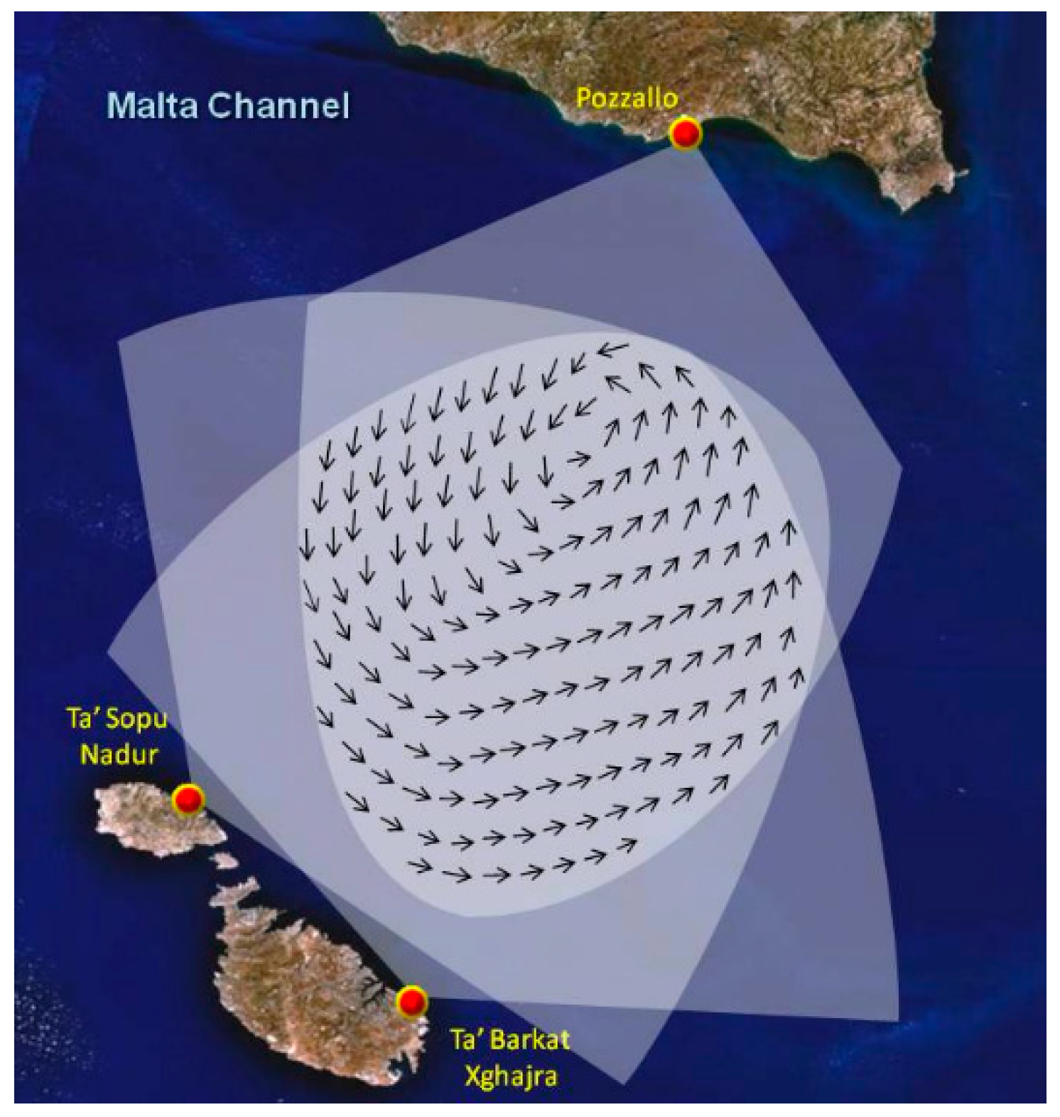
  • HFR data from three CODAR SeaSondes stations installed in Ta’Sopu (Gozo, Malta), Ta’Barkat (Malta) and Pozzallo Harbor (Sicily, Italy) shown in Figure 2, provided surface current maps in the channel from the period August 2012 to January 2015. These data correspond to a setup of two HFR stations initially installed at Ta’Sopu and Ta’Barkat in August 2012. The third station was added in August 2013 in Pozzallo improving the spatial coverage of the channel [26]. The data are organized in time series of hourly velocity vectors with u (zonal, East-West) and v (meridional, North-South) components of the total velocity. The datasets were based on CALYPSO HFR, compiled and processed by Dr. Simone Cosoli from the University of Western Australia, Perth [27]. The CALYPSO system operating set-up and resolution (13.5 MHz frequency, angular resolution 5°, range resolution 1.6 km, for more details see Drago et al. [10]) provides radar measurements that are representative of the first meter of the ocean with grid sizes from 0.3 to 8.3 km2. The radars share the same transmit frequency using a GPS-synchronization module and operate with both the ideal and measured antenna beam patterns. Hourly sea surface current maps were derived on a Cartesian grid with 3 × 3 km2 horizontal resolution by least-squares fitting of the radial components of the ocean currents from two or more radar stations in areas of common overlap. Grid points were included in the analysis only if they satisfied a minimum data return of 50% using an interpolation technique described in Cosoli et al. [27]. Validation of this array has been carried out in different studies since the installation of the system making this dataset a reliable product [27,28,29].
  • Ssalto/Duacs multi-mission L4 altimeter products in the period January 1993 to December 2015 containing daily multi-mission ADT on a 1/8° × 1/8° mercator projection grid, and distributed by the Copernicus Marine and Environment Monitoring Service (CMEMS) [4,5,31] were used to calculate SGV where,
    u g = g f ζ y ,
    v g = g f ζ x .
    are the zonal and meridional geostrophic velocities, and ζ, denotes the dynamic topography provided by the altimeter.
  • Monthly Level-3 binned SST [doi: 10.5067/AQUA/MODIS/L3M/SST/2014] and CHL [doi: 10.5067/AQUA/MODIS/L3B/CHL/2018] datasets with a spatial resolution of 4.6 km were downloaded from January to December 2013 from the OceanColor web portal (https://oceandata.sci.gsfc.nasa.gov/MODIS-Aqua/Binned/Monthly/) under the NASA aqua-MODIS (Moderate Resolution Imaging Spectroradiometer) satellite mission.
  • A sub-grid ranging from 35.8–36.8° N to 13.8–15.4° E from the six-hourly gridded Cross-Calibrated Multi-Platform (CCMP) V2.0, Remote Sensing Systems (RSS), Santa Rosa, California, USA. Level-3 wind vector analyses product was downloaded from Remote Sensing Systems (RSS) for the period spanning August 2013 to January 2015 to analyze wind patterns in the channel [32]. The CCMP dataset combines cross-calibrated satellite microwave winds from scatterometers and radiometers with instrument observations using a variational analysis method to produce 1/4° gridded data [33]. Both radiometer and scatterometer data are validated against ocean moored buoys (in agreement within 0.8 m/s), where wind observations are referenced to a height of 10 m. For a complete description of the dataset see [32].

2.2. Complex Correlation and Veering Estimates

Average veering between two 2D time series can be obtained from the phase angle of the complex correlation coefficient [34]. Additionally, we used this method to determine if the wind and HFR velocities are in Ekman Balance.
Let,
w ( t ) = u ( t ) + i v ( t ) ,
be the complex representation of the velocity time series at time t. The complex correlation coefficient between the two vector time series 1 and 2 in terms of the east and west components is:
p = u 1   u 2 + v 1   v 2 u 1 2 + v 1 2 1 2   u 2 2 + v 2 2 1 2 + i u 1   v 2 u 2   v 1 u 1 2 + v 1 2 1 2   u 2 2 + v 2 2 1 2   ,
where the phase angle or average veering is,
α a v = u 1   v 2 u 2   v 1 u 1   u 2 + v 1   v 2 .

2.3. Kinematic Properties of an Eddy

In order to describe the channel in terms of its kinematic properties, we applied the method described by Sanderson [35] using the lstranslate routine developed by the HFR group at the Naval Postgraduate School.
Assuming there is an eddy linearly translated in time with spatially uniform velocity gradients as follows:
g 11 =   u x
g 12 =   u y
g 21 =   v x
g 22 =   v y
From Equations (6)–(9), the divergence is defined as d = g 11 + g 22 , stretching deformation a = g 11 g 22 , vorticity c = g 21 g 12 and the shearing deformation b = g 21 + g 12 , which are functions of the velocity gradients. The method assumes that the center of the eddy is located at X, Y and moves with constant velocity (U, V), whereas, at some distance from the center of the eddy, the flow velocity has an added component due to the velocity gradients. X0, Y0 is defined as the initial position of the eddy. Then the flow center position can be written as,
X = X 0 + U ( t ) ,
Y = Y 0 + V ( t ) .
with,
α = U g 11 X 0 g 12 Y 0 ,
β = V g 21 X 0 g 22 Y 0 ,
α 1 = g 11 U g 12 V ,
β 1 = g 21 U g 22 V .
and solving Equations (12)–(15) for U, V, X0, Y0 yields,
U = g 22 α 1 g 12 β 1 g 12 g 21 g 11 g 22
V = g 11 β 1 g 21 α 1 g 12 g 21 g 11 g 22
X 0 = g 22 ( α U ) g 12 ( β V ) g 12 g 21 g 11 g 22
Y 0 = g 11 ( β V ) g 21 ( α U ) g 12 g 21 g 11 g 22
For our studies, we focused on the vorticity component applied to the HFR data in order to quantitatively identify the mesoscale features within the study area.

3. Results and Discussion

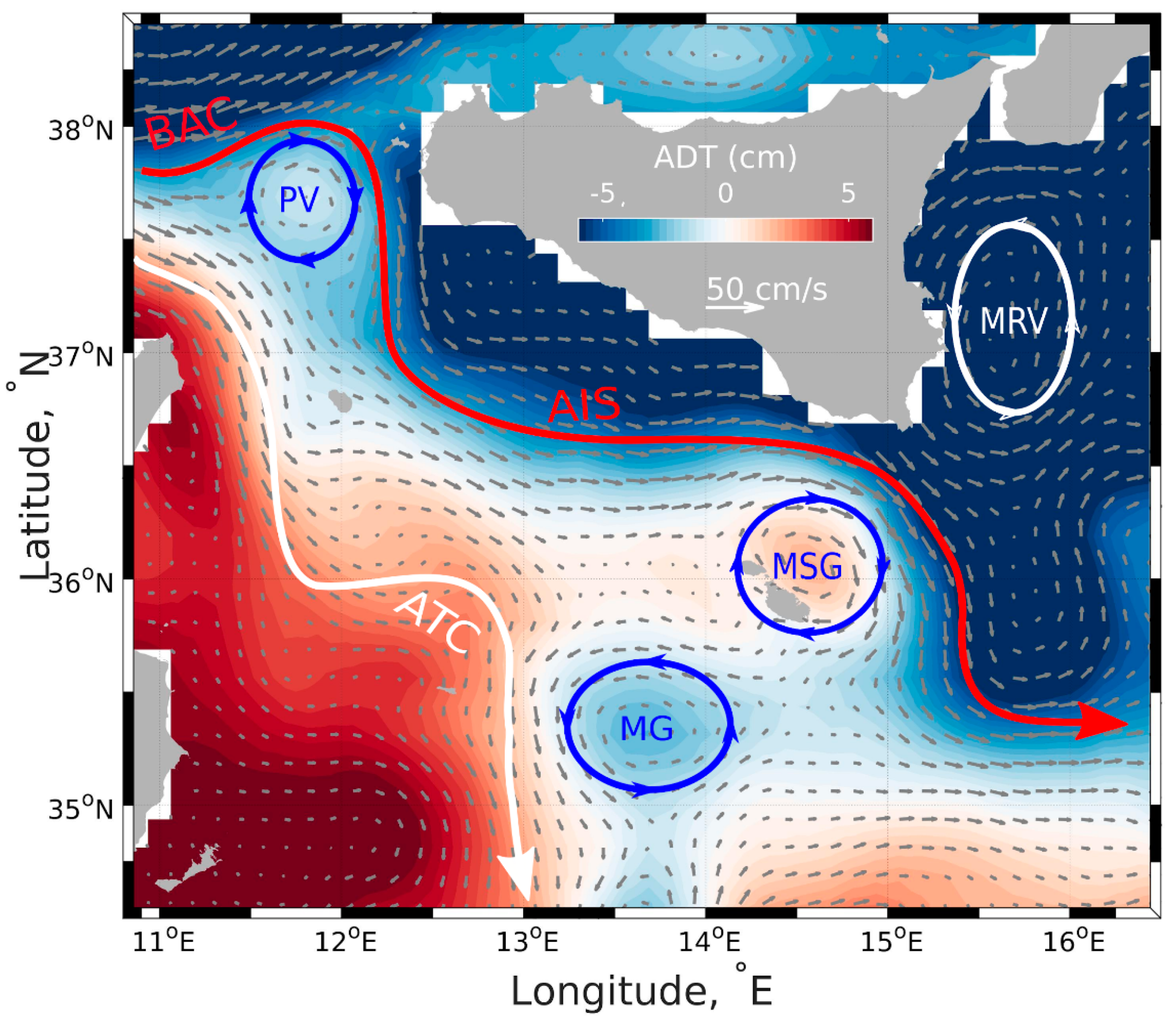
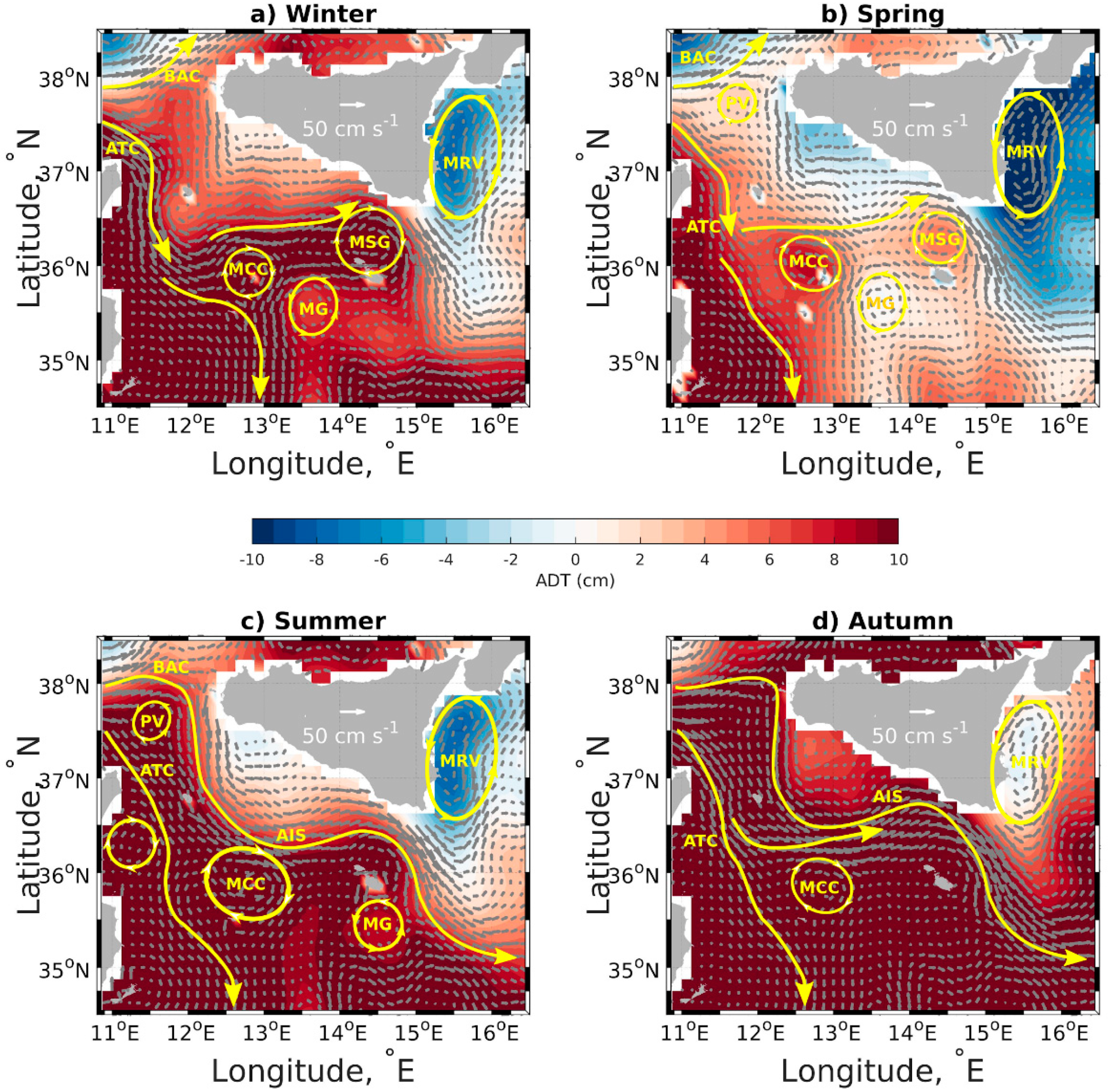
3.1. Mean Surface Circulation, the Sicily Channel

Due to baroclinic instabilities, the Atlantic current (AC) regularly forms meanders that eventually detach from the current and become either cyclonic or anticyclonic eddies [36] like the ones observed by Jouini et al. [3] and Jebri et al. [37,38]. Figure 3 shows the SC inter-annual geostrophic circulation derived from the ADT data depicting some of the AC-born structures described in Jouini et al. [3] and Menna et al. [5] such as the cyclonic Medina Gyre (MG), the cyclonic Messina Rise Vortex (MRV), the anticyclonic Pantelleria Vortex (PV, which in the literature is mentioned as cyclonic), the anticyclonic MSG, the AIS, the Bifurcation Atlantic Current (BAC) and the Atlantic Tunisian Current (ATC). From ADT and SGV, the MSG shows a seasonal semi-permanent behavior and contributes to the channel’s circulation along with the AIS. Due to its poor description in the literature its characterization is an important result of our studies. The complex bathymetry in the SC, with its longitudinal subdivision into two sills, influences the distribution of ADT leading to a difference in level between the two sides of the channel as seen in Figure 3. Towards the Italian side the sea level is lower than on the Tunisian side with a dipole like sea level shape, positive ADT close to Tunisia and negative towards Sicily.
The seasonal variability of the circulation in Figure 4 was obtained by averaging the ADT maps using the following groupings: Winter (December, January, February), Spring (March, April, May), Summer (June, July, August) and Autumn (September, October, November). In winter (Figure 4a) the mean geostrophic circulation shows the presence of the AC bifurcating at the SS in two branches due to the two-sill bathymetry of the strait. The BAC flows toward the northern tip of Sicily while the ATC to the Tunisian side. The MSG is observed as well with a radius of ~50 km and centered at 14.5°E–36.1°N. It is also prominent during the winter/spring season as seen in Figure 4b, dominating the circulation in the channel when the AIS is not present. This can be interpreted as a result of the conservation of potential vorticity [13,14,15] since the water depth abruptly changes from ~700 m at the Malta graben to shallow (~100 m) in the channel (see Figure 1). For this season, the MSG velocity ranges between 5–10 cm s−1. Additionally, other structures observed for this season are the anticyclonic MCC, the cyclonic MG and MRV.
In spring we identify some of the winter structures indicated in Jouini et al. [3] and Menna et al. [4,5] like the ATC, BAC, MCC, MG, MSG, MRV and the PV as shown in Figure 4b. The ATC flows towards Sicily where two gyres are detached, the cyclonic MG and the anticyclonic MCC circling around Linosa island, most likely due to the influence of the LT at 36°N. In addition, at the northern tip of Sicily there is a re-circulation of AW that enters into the SC where the PV is detached and the MSG is reinforced.
For the summer period we observe the strong influence of the AIS (Figure 4c) which behaves like a jet stream in the SC and the channel [13]. It is characterized by a velocity of ~25 cm s−1 and occasionally reaching values higher than 50 cm s−1. This current consists mainly of AW and changes properties as it passes through the SS deepening and bifurcating into the Ionian Sea northwards or to the Central Ionian Sea depending on the NIG phase [19,21,23,38]. Additionally, the ADT and SGV also show another yet unidentified mesoscale structure close to the coast of Tunisia detached from the ATC, and a shift of the MG eastwards.
Figure 4d shows autumn mean geostrophic circulation which is driven by the AIS and reinforced by AW coming from the BAC and the ATC. The ATC bifurcates at the SS and then rejoins south of Pantelleria. We observed other mesoscale structures, like the cyclonic MRV and the anticyclonic MCC, as well as the formation of the anticyclonic MSG which has been undocumented in the literature.
Other permanent structures were found in the SC in disagreement with the current literature. For example, the anticyclonic PV at 37.5°N–11.5°E is in disagreement with the studies of Robinson et al. [12], Lermusiaux and Robinson. [15] and Jouini et al. [3]. In their case the PV is cyclonic and positioned at 37°N–12°E. Additionally, the MCC is described as a summer only pattern in the literature but in our studies is also present in winter and spring. The cyclonic Adventure Bank Vortex (ABV) and the ISV were summer only structures in the literature but were not found in our seasonal or inter-annual geostrophic decomposition. Furthermore, over the monthly mean analysis we were able to identify some of these structures, but they seemed to be temporary and appeared just in some years/months where they could have been triggered by rare and strong atmospheric events. An updated picture of the surface circulation structures in the whole SC where the discrepancies and the reasons why they are enhanced should be clarified and studied with more extent and detail. A new study of all these structures and the forcing mechanisms behind them can be found in Menna et al. [5], but again the MSG is not mentioned.
Wind stress curl and deseasonalized geostrophic eddy kinetic energy (EKE) studies in Menna et al. [4] revealed the influence of the wind and highlights the regions with high EKE in the Central Mediterranean Sea. Wind stress data (Figure 3c,d in Menna et al. [4]) shows that towards the southwestern side of the Sicilian coast northwesterly winds favor upwelling (+ wind stress) revealing persistent coastal Ekman pumping events [39,40]. Wind forcing imparts an indirect influence in the current field at longer time scales (weekly, monthly, and inter-annual), where even if neglected in the geostrophic approximation, helps to build up the sea level to generate a sufficiently large pressure gradient needed to balance the Coriolis force. On the other hand, deseasonalized geostrophic EKE studies (Figure 6 in Menna et al. [4]) highlight areas in the central Mediterranean Sea where the inter-annual variability is stronger with values of ~80 cm2 s−2 in the channel. A broader EKE variability using altimetry and model datasets in the Mediterranean Sea can be found in Pujol and Larnicol [41] and Jordi and Wang [42].

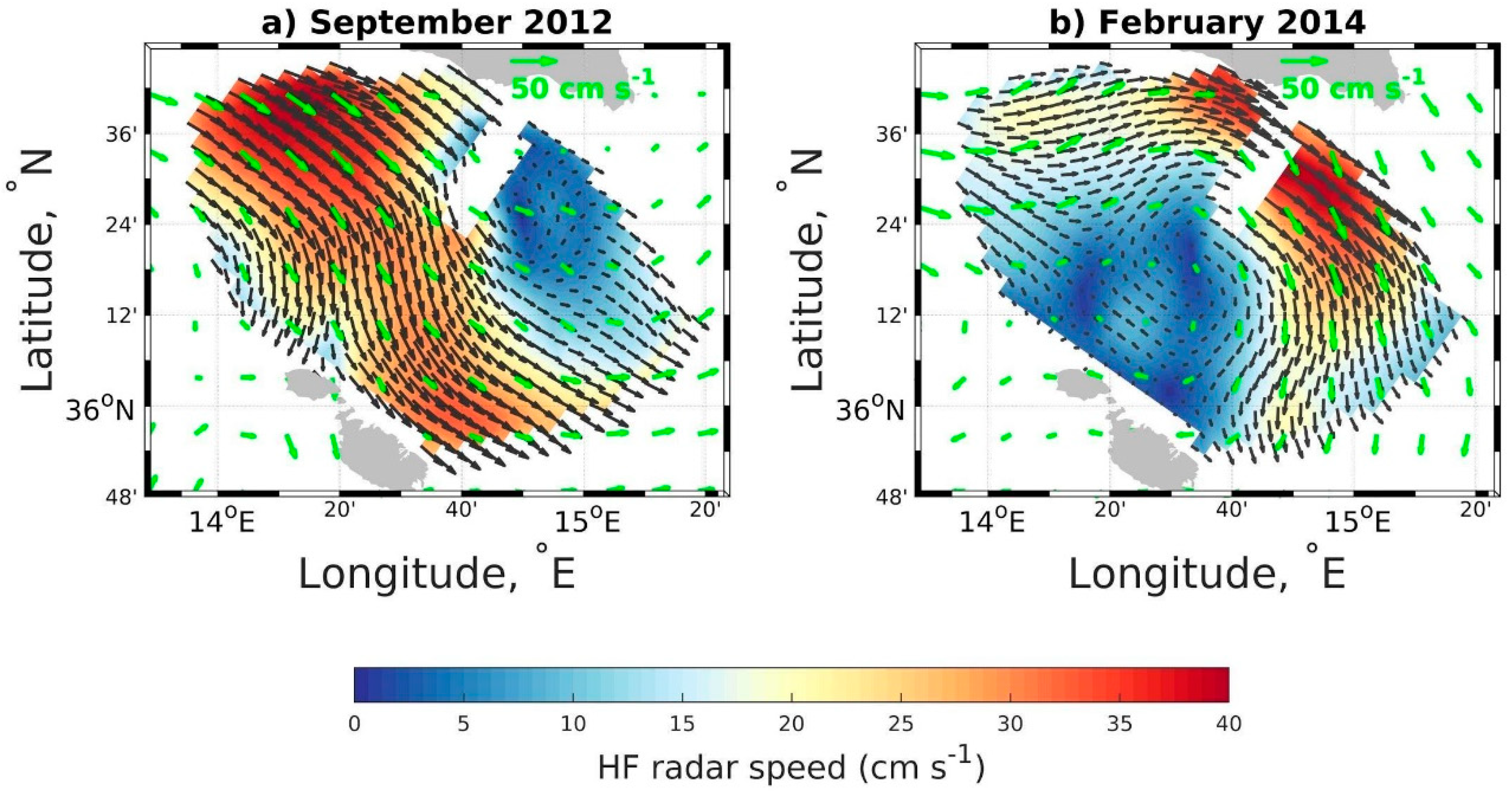
3.2. Short Time Scales in the Malta Sicily Channel

3.2.1. Comparison among Available Spatial Data

Ocean currents can be described as a combination of geostrophic and ageostrophic terms, the latter being associated with wind driven features. HFRs offer good resolution in both time and space, and have the capability to measure near real-time complete currents [43,44], measuring both wind-driven and geostrophic components influencing the sea surface. Weekly, monthly, inter-annual and seasonal averages of SGV and HFR velocity field were compared. Figure 5 shows monthly means of both components correlate well geographically. This strong correlation was found at all-time scales greater than a day and thus identified the channel to be in geostrophic balance at these time scales. As expected, the stretching and squeezing of the anticyclonic MSG and the AIS jet stream were also observed from the HFR data as did the SGV and ADT. In addition, the MSG can occasionally have velocities as high as 40 cm s−1 as seen in Figure 5b.
Other spatial observations available for this area include monthly satellite derived SST and CHL data, which were compared with HFR monthly averages for the period from January to December 2013. Since the prevailing signal in the HFR data at monthly time scales is geostrophic, it is expected that the advection of properties follows this flow. However, one should remember that SST and CHL are not conservative tracers but can be used in general to track currents, circulation, and water mass mixing among other properties. Figure 6a,c show SST and CHL maps in January 2013 respectively, revealing relatively higher temperatures and lower CHL occupying the channel and lower temperatures and higher CHL constrained towards the Sicilian coast. This behavior can be associated with the presence of the MSG, which for the winter season is the predominant pattern. Figure 6b,d illustrate that as the AIS flows towards the Ionian Sea it generates a well-defined front which advects properties in the channel along its path [12]. Additionally, the SST field varies from 17 °C to 26 °C while CHL from 0.5 to 0.05 mg m−3 through winter to the end of summer. A detailed statistical analysis of CHL and SST data is presented in Capodici et al. [26].

3.2.2. Complex Correlation

We spatially averaged wind (1/4°), SGV (1/8°) and HFR (1 km) daily gridded data to match the 1/4° wind grid. Figure 7 shows the spatially averaged time series over the 1/4° grid for each dataset. The comparison of the three parameters in panels a and c of Figure 7 show that the geostrophic components (u,vSGV) behave like a low-pass filter of the HFR time series because the geostrophic adjustment takes place on a longer time scale. Wind (u,vwind) and HFR (u,vradar) time series show most of the high frequency motions included at short time scales, where the wind plays an important role on the channel circulation. Additionally, panels b and d compare the wind speed time series with the residual velocity obtained by removing the geostrophic component from the HFR data, u,vresidual = u,vradaru,vSGV, where the residual is expected to be better correlated to the wind components than to the geostrophic current. Here the u component (panel b) shows good agreement with the residual as expected, except for some time intervals such as January to March 2013 where the wind is positive and the residual is negative and higher in magnitude. The residual meridional v component of the velocity (panel d) behaves differently from the wind signal in the first few months (until September 2013). This is probably due to data availability since for some grid cells the lack of HFR data could play an important role in the magnitude of the vectors and thus the averaging process.
In order to look for the relationship between different variables, we compute the vector correlation between the interpolated time series in Figure 7 over the grid represented in Figure 8 where the boxes represent the 1/4° grid defined previously. HFR to the wind complex correlation (as seen in Table 2) shows the veering 43.5781 ± 8.238 degrees to the right, in a good agreement with theory. The angles of the velocity to the wind vector varies between 23 to 53 degrees with a range correlation between 0.24 to 0.35, showing the importance of the wind forcing at shorter time scales and in the set-up of the Ekman layer. The correlation between the residual current and the wind vector is higher than the radar to wind correlation. The angles between residual and wind are closer to 45 degrees, as a result of the removal of the geostrophic components from the time series (see Table 2). Finally, as expected the complex correlation between the geostrophic flow and the wind is very low since processes in both time series evolve at different time scales; the wind component at short time scales generate rapid and variable motions (i.e., inertial oscillations) in the ocean whereas the geostrophic field evolves at larger scales accounting for low frequency phenomena.

3.3. The Malta Sicily Gyre

Evidence of mesoscale activity in the channel was highlighted by four datasets considered in this study: ADT, HFR, CHL and SST. To identify this mesoscale activity, we computed the vorticity using the method described in Sanderson [35] considering only a subset of the HFR time series, using the high resolution and continuity criteria. For the continuity criteria we defined the area in Figure 9e where data was available since the start of acquisition. This area also coincides with the place where the MSG was identified with the HFR velocities and geostrophic current analysis.
Figure 9 (panel b and d) shows the presence of the anticyclonic MSG in winter between December-March 2013 and December-August 2014, corroborated by a vorticity of c = −2 × 10⁻⁵ s−1 using Sanderson’s method (panel b and c). These results are in agreement with the winter/spring recurrence of the MSG identified with the ADT and SGV analysis. Here we also note that the MSG co-existed with the AIS from April to August 2014 (shaded areas in Figure 9). This provides a quantitative description of the gyre. Finally, with this method we were able to identify other mesoscales gyres that were either cyclonic (+vorticity) or anticyclonic (−vorticity). Some examples are depicted in Figure 10.

4. Summary and Conclusions

The main focus of this paper has been to characterize the channel circulation, which was done using satellite-derived geostrophic currents HFR-derived currents, and wind vector analyses on daily time scales in addition to SST and CHL on monthly time scales. Analyzing the available data, with particular emphasis on the higher spatial and temporal resolution of the HFR observations, the MSG is studied in more detail. This is an anticyclonic structure occupying a substantial portion of the channel that has been poorly studied and often confused with the ISV or the MCC. We believe that the standardization of the names and characteristics for these structures will benefit researchers and resource managers working in the region. Menna et al. [5] provides a good description of the main surface circulation structures in the SC but characterizes the MSG (or MCC as they called it) as a seasonal feature, occurring in the summer only. This creates some discrepancies since based on the lower frequency qualitative studies (i.e., SGV, SST and CHL maps), that agree with [10], the mesoscale feature is present mostly in the winter-spring period. This however is not always the case since in 2014 both the AIS and the MSG were present from January to August. Tracking the anticyclonic MSG was particularly well done using the vorticity analysis performed on the HFR observations. While the channel-scale MSG was dominant, other cyclones and anticyclones were identified at daily time scales in the HFR observations making Sanderson’s method a good tool for identifying mesoscale features. A longer HFR time series with better spatial coverage can be useful to study the mesoscale.
Geostrophic balance was found to be a good approximation to describe the dynamics in the channel at weekly, monthly, seasonal and inter-annual time scales. At these time scales, wind forcing is important for creating the density gradients and the subsequent geostrophic velocities, but wind data are not essential in diagnosing the circulation patterns (wind stress curl as in Menna et al. [4], shows persistent coastal Ekman upwelling events along the coast of Sicily.) The geostrophic velocity field in the channel is reinforced by the wind, which is mostly northwest and is responsible for the advection of different properties in the area. At short time scales (hours to days) we were able to use the combination of HFR and geostrophic velocities to show that direct wind forcing must be accounted for. The vector complex correlation between the HFR and the wind time series allowed us to show that the high frequency components included an Ekman balance between wind and surface current. The analysis showed a veering angle for the currents of 43.5781 ± 8.238 degrees to the right of the wind forcing, which is in good agreement with Ekman theory. The agreement was even better when the geostrophic currents were subtracted from the HFR observations to produce a residual current. Hence, we conclude that HFR observations or a wind-based correction to the geostrophic currents, are recommended at daily time scales. This set of analyses using observations at larger time and space scales from satellites and observations of higher frequency, higher resolution features from HFR suggests that this suite of observations can provide effective monitoring of the circulation state for important regions, such as the area studied here.

Author Contributions

Writing—original draft, N.C.R.S.; Writing—review & editing, N.C.R.S., M.S.C., M.G., J.D.P., A.D. and V.C.; Conceptualization, N.C.R.S., M.S.C., M.G. and J.D.P.; Data curation, N.C.R.S. and M.S.C.; Formal analysis, N.C.R.S., M.S.C. and J.D.P.; Funding acquisition, A.D., M.G. and V.C.; Investigation, N.C.R.S. and M.G.; Methodology, N.C.R.S., M.G. and J.D.P.; Resources, M.G., A.D. and V.C.; Software, M.S.C. and J.D.P.; Supervision, M.S.C., M.G. and J.D.P; Visualization, N.C.R.S.

Funding

This research was financially supported through the award of the scholarship to N.C.R.S. by the Istituto Nazionale di Oceanografia e Geofisica Sperimentale—OGS, the University of Trieste—UNITS and the TRIL program of the Abdus Salam International Center for Theoretical Physics—ICTP. HF radar data were collected within the Italia-Malta program-Cohesion Policy 2007–2013, European Union regional Development Funds (ERDF) through the CALYPSO project.

Acknowledgments

The authors would like to thank Aldo Drago for providing the HFR data used in this study. We also acknowledged Simone Cosoli for providing the processed and QC dataset from the HFR array. Last but not least, we also thank to the two anonymous reviewers for their constructive observations.

Conflicts of Interest

The authors declare no conflict of interest.

Abbreviations

The following abbreviations are used in this manuscript:
Currents
ACAtlantic Current
ATCAtlantic Tunisian Current
AISAtlantic Ionian Stream
BACBifurcation Atlantic/Algerian current
MIJMid-Ionian Jet
Water Masses
AWAtlantic Water
Geographical Names
ABAdventure Bank
MPMalta Plateau
GBGela Basin
MTMalta Trough
LaLampedusa
PPantelleria
LiLinosa
PTPantelleria Trough
LTLinosa Trough
SSicily
MMaltese Islands
SCSicily Channel
ChannelMalta-Sicily Channel
SMESicily-Malta Escarpment
MBMedina Bank
SSSicily Strait
TPTunisia Plateau
Gyres
ABVAdventure Bank Vortex (Cyclonic)
MRVMesina Rise Vortex (Cyclonic)
ISVIonian Shelf Break Vortex (Cyclonic)
MSGMalta-Sicily Gyre (Anticyclonic)
MCCMalta Channel Crest (Anticyclonic)
MGMedina Gyre (Cyclonic)
NIGNorth Ionian Gyre (Cyclonic/Anticyclonic)
PVPantelleria vortex (Anticyclonic)
Datasets
CCMPCross-Calibrated Multi-Platform wind vector analysis
CMEMSCopernicus Marine and Environment Monitoring Service
CODARCoastal ocean dynamics applications radar
HFRHigh Frequency Radar
MODISModerate Resolution Imaging Spectroradiometer
NASANational Aeronautics and Space Administration
NOAAThe National Oceanic and Atmospheric Administration
NSFNational Science Foundation
RSSRemote sensing systems (scientific company)
Physical Properties
ADTAbsolute Dynamic Topography
CHLSatellite Sea surface chlorophyll concentrations
EKEEddy Kinetic Energy
SGVSurface Geostrophic Velocity
SSTSatellite Sea Surface Temperature

References

  1. Robinson, A.R.; Leslie, W.G.; Theocharis, A.; Lascaratos, A. Encyclopedia of Ocean Sciences: Mediterranean Sea Circulation, 2nd ed.; Academic London: London, UK, 2001; Volume 3, pp. 1689–1705. [Google Scholar] [CrossRef]
  2. Malanotte-Rizzoli, P.M.; Robinson, A.R. Ocean Processes in Climate Dynamics: Global and Mediterranean Examples; Springer Science & Business Media: Berlin, Germany, 2012; Volume 419. [Google Scholar] [CrossRef]
  3. Jouini, M.; Béranger, K.; Arsouze, T.; Beuvier, J.; Thiria, S.; Crépon, M.; Taupier-Letage, I. The Sicily Channel surface circulation revisited using a neural clustering analysis of a high-resolution simulation. J. Geophys. Res. Oceans 2016, 121, 4545–4567. [Google Scholar] [CrossRef]
  4. Menna, M.; Reyes-Suarez, N.C.; Civitarese, G.; Gačić, M.; Poulain, P.-M.; Rubino, A. Decadal variations of circulation in the Central Mediterranean and its interactions with the mesoscale gyres. Deep Sea Res. Part II Top. Stud. Oceanogr. 2019. [Google Scholar] [CrossRef]
  5. Menna, M.; Poulain, P.-M.; Ciani, D.; Doglioli, A.; Notarstefano, G.; Gerin, R.; Rio, M.H.; Santoleri, R.; Gauci, A.; Drago, A. New insights of the Sicily Channel and southern Tyrrhenian Sea variability. Water 2019, 11, 1355. [Google Scholar] [CrossRef]
  6. Würtz, M.; Rovere, M. Atlas of the Mediterranean Seamounts and Seamount-Like Structures; IUCN: Grand, Switzerland, 2015. [Google Scholar]
  7. Ismail, S.B.; Schroeder, K.; Sammari, C.; Gasparini, G.P.; Borghini, M.; Aleya, L. Interannual variability of water mass properties in the Tunisia–Sicily Channel. J. Mar. Syst. 2014, 135, 14–28. [Google Scholar] [CrossRef]
  8. Lodolo, E.; Ben-Avraham, Z. A submerged monolith in the Sicilian Channel (central Mediterranean Sea): Evidence for Mesolithic human activity. J. Archaeol. Sci. Rep. 2015, 3, 398–407. [Google Scholar] [CrossRef]
  9. Drago, A.; Azzopardi, J.; Gauci, A.; Tarasova, R.; Ciraolo, G.; Capodici, F.; Gačić, M. Sea surface currents by HF radar in the Malta channel. Rapp. Comm. Int. Mer Medit. 2013, 40, 144. [Google Scholar]
  10. Drago, A.; Ciraolo, G.; Capodici, F.; Cosoli, S.; Gačić, M.; Poulain, P.-M.; Tarasova, R.; Azzopardi, J.; Gauci, A.; Maltese, A.; et al. CALYPSO—An operational network of HF radars for the Malta-Sicily Channel. In Proceedings of the 7th International Conference on EuroGOOS, Lisbon, Portugal, 28–30 October 2014; Volume 30, pp. 28–30. [Google Scholar]
  11. Smith, W.H.F.; Sandwell, D.T. Global seafloor topography from satellite altimetry and ship depth soundings. Science 1997, 277, 1957–1962. [Google Scholar] [CrossRef]
  12. Robinson, A.R.; Sellschopp, J.; Warn-Varnas, A.; Leslie, W.G.; Lozano, C.J.; Haley, P.J., Jr.; Anderson, L.A.; Lermusiaux, P.F.J. The Atlantic Ionian Stream. J. Mar. Syst. 1999, 20, 129–156. [Google Scholar] [CrossRef]
  13. Drago, A.; Sorgente, R.; Olita, A. Sea Temperature, Salinity and Total Velocity Climatological Fields for the South-Central Mediterranean Sea. MedSudMed Technical Documents Gcp/Rer/010/Ita/Msm-Td-14. 2010, 35. No. 14. Available online: http://www.faomedsudmed.org/html/doc/Publication_issue.asp?id=195 (accessed on 30 July 2019).
  14. Lermusiaux, P.F.J. Estimation and study of mesoscale variability in the Strait of Sicily. Dyn. Atmos. Oceans 1999, 29, 255–303. [Google Scholar] [CrossRef]
  15. Lermusiaux, P.F.J.; Robinson, A.R. Features of dominant mesoscale variability, circulation patterns and dynamics in the Strait of Sicily. Deep Sea Res. Part I Oceanogr. Res. Pap. 2001, 48, 1953–1997. [Google Scholar] [CrossRef]
  16. Béranger, K.; Mortier, L.; Gasparini, G.P.; Gervasio, L.; Astraldi, M.; Crépon, M. The dynamics of the Sicily Strait: A comprehensive study from observations and models. Deep Sea Res. Part II Top. Stud. Oceanogr. 2004, 51, 411–440. [Google Scholar] [CrossRef]
  17. Robinson, A.R.; Malanotte-Rizzoli, P.; Hecht, A.; Michelato, A.; Roether, W.; Theocharis, A.; Ünlüata, Ü; Pinardi, N.; Artegiani, A.; Bergamasco, A.; et al. General circulation of the Eastern Mediterranean. Earth-Sci. Rev. 1992, 32, 285–309. [Google Scholar] [CrossRef]
  18. Pinardi, N.; Zavatarelli, M.; Adani, M.; Coppini, G.; Fratianni, C.; Oddo, P.; Simoncelli, S.; Tonani, M.; Lyubartsev, V.; Dobricic, S.; et al. Mediterranean Sea large-scale low-frequency ocean variability and water mass formation rates from 1987 to 2007: A retrospective analysis. Prog. Oceanogr. 2015, 132, 318–332. [Google Scholar] [CrossRef]
  19. Gačić, M.; Borzelli, G.E.; Civitarese, G.; Cardin, V.; Yari, S. Can internal processes sustain reversals of the ocean upper circulation? The Ionian Sea example. Geophys. Res. Lett. 2010, 37. [Google Scholar] [CrossRef]
  20. Gačić, M.; Civitarese, G.; Eusebi Borzelli, G.L.; Kovačević, V.; Poulain, P.M.; Theocharis, A.; Menna, M.; Catucci, A.; Zarokanellos, N. On the relationship between the decadal oscillations of the northern Ionian Sea and the salinity distributions in the eastern Mediterranean. J. Geophys. Res. Oceans 2011, 116. [Google Scholar] [CrossRef]
  21. Gačić, M.; Schroeder, K.; Civitarese, G.; Cosoli, S.; Vetrano, A.; Eusebi Borzelli, G.L. Salinity in the Sicily Channel corroborates the role of the Adriatic–Ionian Bimodal Oscillating System (BiOS) in shaping the decadal variability of the Mediterranean overturning circulation. Ocean Sci. 2013, 9, 83–90. [Google Scholar] [CrossRef]
  22. Civitarese, G.; Gačić, M.; Lipizer, M.; Eusebi Borzelli, G.L. On the impact of the Bimodal Oscillating System (BiOS) on the biogeochemistry and biology of the Adriatic and Ionian Seas (Eastern Mediterranean). Biogeosciences 2010, 7, 3987–3997. [Google Scholar] [CrossRef] [Green Version]
  23. Bessières, L.; Rio, M.H.; Dufau, C.; Boone, C.; Pujol, M.I. Ocean state indicators from MyOcean altimeter products. Ocean Sci. 2013, 9. [Google Scholar] [CrossRef]
  24. Sammari, C.; Millot, C.; Taupier-Letage, I.; Stefani, A.; Brahim, M. Hydrological characteristics in the Tunisia–Sardinia–Sicily area during spring 1995. Deep Sea Res. Part I Oceanogr. Res. Pap. 1999, 46, 1671–1703. [Google Scholar] [CrossRef]
  25. Ciappa, A.C. Surface circulation patterns in the Sicily Channel and Ionian Sea as revealed by MODIS chlorophyll images from 2003 to 2007. Cont. Shelf Res. 2009, 29, 2099–2109. [Google Scholar] [CrossRef]
  26. Capodici, F.; Ciraolo, G.; Cosoli, S.; Maltese, A.; Mallandrino, G. The synergy of water quality and sea surface currents data in determining the spatio-temporal evolution of large-scale circulation features. In Remote Sensing for Agriculture, Ecosystems, and Hydrology XVI; International Society for Optics and Photonics: Amsterdam, The Netherlands, 2014; Volume 9239, p. 923927. [Google Scholar] [CrossRef]
  27. Cosoli, S.; Drago, A.; Ciraolo, G.; Capodici, F. Tidal currents in the Malta–Sicily Channel from high-frequency radar observations. Cont. Shelf Res. 2015, 109, 10–23. [Google Scholar] [CrossRef]
  28. Gauci, A.; Drago, A.; Abela, J. Gap Filling of the CALYPSO HF Radar Sea Surface Current Data through Past Measurements and Satellite Wind Observations. Int. J. Navig. Obs. 2016. [Google Scholar] [CrossRef]
  29. Capodici, F.; Cosoli, S.; Ciraolo, G.; Nasello, C.; Maltese, A.; Poulain, P.M.; Drago, A.; Azzopardi, J.; Gauci, A. Validation of HF radar sea surface currents in the Malta-Sicily Channel. Remote Sens. Environ. 2019, 225, 65–76. [Google Scholar] [CrossRef]
  30. CALYPSO: Real-Time Viewing of Sea Surface Currents in the Malta Channel. Available online: http://www.mongoos.eu/-/calypso-real-time-viewing-of-sea-surface-currents-in-the-malta-channel (accessed on 4 July 2018).
  31. Rio, M.H.; Pascual, A.; Poulain, P.M.; Menna, M.; Barceló, B.; Tintoré, J. Computation of a new mean dynamic topography for the Mediterranean Sea from model outputs, altimeter measurements and oceanographic in situ data. Ocean Sci. 2014, 10, 731–744. [Google Scholar] [CrossRef] [Green Version]
  32. Wentz, F.J.; Scott, J.; Hoffman, R.N.; Leidner, S.M.; Atlas, R.; Ardizzone, J. Remote Sensing Systems Cross-Calibrated Multi-Platform (CCMP) 6-Hourly Ocean Vector Wind Analysis Product on 0.25 deg Grid, Version 2.0, [Aug 2013–Jan 2015]. Remote Sensing Systems: Santa Rosa, CA. Available online: www.remss.com/measurements/ccmp (accessed on 5 December 2017).
  33. Atlas, R.; Hoffman, R.N.; Ardizzone, J.; Leidner, S.M.; Jusem, J.C.; Smith, D.K.; Gombos, D. A cross-calibrated, multiplatform ocean surface wind velocity product for meteorological and oceanographic applications. Bull. Am. Meteorol. Soc. 2011, 92, 157–174. [Google Scholar] [CrossRef]
  34. Kundu, P.K. Ekman veering observed near the ocean bottom. J. Phys. Oceanogr. 1976, 6, 238–242. [Google Scholar] [CrossRef]
  35. Sanderson, B.G. Structure of an eddy measured with drifters. J. Geophys. Res. Oceans 1995, 100, 6761–6776. [Google Scholar] [CrossRef]
  36. Malanotte-Rizzoli, P.; Artale, V.; Borzelli-Eusebi, G.L.; Brenner, S.; Crise, A.; Gačić, M.; Kress, N.; Marullo, S.; Ribera d’Alcalà, M.; Sofianos, S.; et al. Physical forcing and physical/biochemical variability of the Mediterranean Sea: A review of unresolved issues and directions for future research. Ocean Sci. 2014, 10, 281–322. [Google Scholar] [CrossRef]
  37. Jebri, F.; Birol, F.; Zakardjian, B.; Bouffard, J.; Sammari, C. Exploiting coastal altimetry to improve the surface circulation scheme over the central Mediterranean Sea. J. Geophys. Res. Oceans 2016, 121, 4888–4909. [Google Scholar] [CrossRef] [Green Version]
  38. Jebri, F.; Zakardjian, B.; Birol, F.; Bouffard, J.; Jullion, L.; Sammari, C. Interannual variations of surface currents and transports in the Sicily channel derived from coastal altimetry. J. Geophys. Res. Oceans 2017, 122, 8330–8353. [Google Scholar] [CrossRef]
  39. Drago, A.; Sorgente, R.; Ribotti, A. A high resolution hydrodynamic 3-D model simulation of the Malta shelf area. Ann. Geophys. 2003, 21, 323–344. [Google Scholar] [CrossRef]
  40. Manzella, G.M.; Gasparini, G.P.; Astraldi, M. Water exchange between the eastern and western Mediterranean through the Strait of Sicily. Deep Sea Res. Part A Oceanogr. Res. Pap. 1988, 35, 1021–1035. [Google Scholar] [CrossRef]
  41. Pujol, M.I.; Larnicol, G. Mediterranean Sea eddy kinetic energy variability from 11 years of altimetric data. J. Mar. Syst. 2005, 58, 121–142. [Google Scholar] [CrossRef]
  42. Jordi, A.; Wang, D.P. Mean dynamic topography and eddy kinetic energy in the Mediterranean Sea: Comparison between altimetry and a 1/16 degree ocean circulation model. Ocean Model. 2009, 29, 137–146. [Google Scholar] [CrossRef]
  43. Paduan, J.D.; Washburn, L. High-frequency radar observations of ocean surface currents. Annu. Rev. Mar. Sci. 2013, 5, 115–136. [Google Scholar] [CrossRef]
  44. Paduan, J.D.; Graber, H.C. Introduction to high-frequency radar: Reality and myth. Oceanography 1997, 10, 36–39. [Google Scholar] [CrossRef]
Figure 1. Bathymetric map of the Sicily Channel (SC) (dashed yellow box) and the channel (solid yellow box) and the surrounding area. Geographical places are indicated with red letters: Adventure Bank (AB), Gela Basin (GB), Lampedusa Island (La), Linosa Island (Li), Linosa Trough (LT), Maltese Islands (M), Malta Plateau (MP), Malta Trough (MT), Medina Bank (MB) Pantelleria Island (P), Pantelleria Trough (PT), Sicily Island (S), Sicily Strait (SS), Sicily-Malta Escarpment (SME), and Tunisia Plateau (TP). The colorbar represents depth in meters. Bathymetric data was obtained from https://topex.ucsd.edu/cgi-bin/get_data.cgi [11].
Water 11 01589 g001
Figure 2. High frequency radar stations of three CODAR SeaSondes stations at Ta’Sopu (Gozo, Malta), Ta’Barkat (Malta) and Pozzallo Harbor (Sicily, Italy) from [30] showing the area of maximum coverage of the array.
Water 11 01589 g002
Figure 3. Inter-annual map of absolute dynamic topography (ADT) and mean surface geostrophic velocities (SGV) in the SC. Permanent structures in white, summer/autumn in red and winter/spring in blue. The colorbar represents the ADT variations over the study area while gray arrows are the SGV vectors.
Water 11 01589 g003
Figure 4. Mean seasonal maps of ADT and SGV in the SC. (a) winter, (b) spring, (c) summer and (d) Autumn. Yellow arrows represent the sea surface patterns found. Gray arrows represent the SGV in cm s−1. The colorbar shows ADT in centimeters.
Water 11 01589 g004
Figure 5. SGV calculated from ADT showing the pathway of Atlantic Ionian Stream (AIS) on September 2012 (left-hand panel) and the Malta-Sicily Gyre (MSG) identified on February 2014 (right-hand panel). Black lines represent monthly averaged current fields derived from high frequency radar data (HFR) data in cm s−1. Green arrows represent SGV in cm s−1. The colorbar gives the magnitude of each velocity vector in cm s−1.
Water 11 01589 g005
Figure 6. Sea surface temperature (SST) and chlorophyll satellite images (CHL) fields from Aqua-MODIS satellite mission showing the MSG on January 2013 (panel (a) and (c), respectively) and the AIS pathway August 2013 (panel (b) and (d), respectively). Gray lines represent monthly averaged surface currents from the HFR, whereas the colorbar represents the SST field in °C (upper panels) and chlorophyll concentration in mg pigment m−3 (lower panels).
Water 11 01589 g006
Figure 7. u and v components of daily wind, SGV and HFR speed time series spatially averaged over a 1/4° grid. Panels (a,c) compare u (zonal, East-West) and v (meridional, North-South) component of the wind (green), SGV (red) and HFR (blue) velocities respectively. Panels (b,d) compare the residual u and v speed (u,vresidual = u,vradaru,vgeostrophic) with u and v components of the wind speed.
Water 11 01589 g007
Figure 8. Grid cells where complex correlation is computed. The subscripts represent the corresponding grid cell for each set of parameters, e.g., p1, θ1 are the parameters corresponding to cell 1.
Water 11 01589 g008
Figure 9. Subset time series of the original HFR grid. Panel (a) represents the u (east-west) while panel (c) the v (north-south) components of the HFR time series respectively. Blue and gray represent the time series respective to the dots on panel (e). Panels (b,d) represent the East-West and North-South differences calculated from the blue time series in panel (a,c) respectively. Vorticity is depicted in the right-hand side of panels (b,d) and was calculated using Sanderson’s method [35]. Violet shaded areas show the months when the MSG was found. Pink shaded areas show the months where the Atlantic Ionian Stream (AIS) and Malta-Sicily Gyre (MSG) co-existed. Green shaded areas show the cyclonic mesoscale in Figure 10c.
Water 11 01589 g009
Figure 10. Daily HFR current maps showing anticyclonic (a,b,d) and cyclonic (c) mesoscale gyres in agreement with the vorticity calculated through Sanderson’s method. The colorbar gives the magnitude of each velocity vector in cm s−1. Please note that panel c depicts one of the cyclonic gyres corresponding to the green shaded areas in Figure 9. Panel a and d depict some of the anticyclonic gyres in the pink shaded areas of Figure 9 occurring alongside the AIS. Panel b shows a snapshot of the MSG in one of shaded violet areas of panels b and d of Figure 9.
Water 11 01589 g010
Table 1. Main characteristics of the remote sensing datasets.
HFRAltimetryMODISMODISCCMP
VariableSea surface velocitiesADT, geostrophic currentsSSTCHL-aWind stress
FrequencyHourlyDailyMonthlyMonthly6-Hourly
Spatial resolution1 km1/8°4.6 km4.6 km1/4°
Vertical integration1 msurfacesurfacesurface10 m above sea level
Study period1 Aug 2012–31 Jan 20151 Jan 1993–31 Dec 2015Jan–Dec 2013Jan–Dec 20131 Aug 2013–31 Jan 2015
Table 2. Shows complex correlation coefficients and veering angles for each time series (high frequency radar data (HFR), surface geostrophic velocities (SGV) and residual) with the wind.
Time SeriesCorrelation CoefficientPhase Angle
Radar to Windp1 = 0.3848θ1 = 34.1950
p2 = 0.3586θ2 = 38.9211
p3 = 0.3515θ3 = 40.1103
p4 = 0.3554θ4 = 23.1126
p5 = 0.3249θ5 = 44.4289
p6 = 0.2475θ6 = 53.4827
p7 = 0.2971θ7 = 33.9368
Residual to Windp1 = 0.4669θ1 = 37.9316
p2 = 0.3749θ2 = 38.9211
p3 = 0.4030θ3 = 49.3575
p4 = 0.4424θ4 = 31.4394
p5 = 0.3145θ5 = 45.5068
p6 = 0.2920θ6 = 59.7371
p7 = 0.3202θ7 = 42.1535
Geostrophic to Windp1 = 0.0566θ1 = −101.4697
p2 = 0.0230θ2 = −14.4575
p3 = 0.1082θ3 = −86.2521
p4 = 0.0876θ4 = −97.4430
p5 = 0.0511θ5 = −34.6377
p6 = 0.0961θ6 = −99.0749
p7 = 0.0712θ7 = −91.4430

