Article

Landslide Susceptibility Mapping Using Different GIS-Based Bivariate Models

1
Young Researchers and Elite Club, Dezful Branch, Islamic Azad University, Dezful 64616-45169, Iran
2
Department of GIS and RS, Faculty of Geography and Planning, University of Tabriz, Tabriz 51666-16471, Iran
3
School of Engineering, University of Guelph, Guelph, ON N1G 2W1, Canada
4
Faculty of Engineering and IT, University of Technology Sydney, Sydney, NSW 2007, Australia
5
Department of Energy and Mineral Resources Engineering, Choongmu-gwan, Sejong University, 209 Neungdong-ro, Gwangjin-gu, Seoul 05006, Korea
6
Institute of Research and Development, Duy Tan University, Da Nang 550000, Vietnam
7
Division of Geoscience Research Platform, Korea Institute of Geoscience and Mineral Resources (KIGAM), 124 Gwahang-no, Yuseong-gu, Daejeon 305-350, Korea
8
Korea University of Science and Technology, 217 Gajeong-roYuseong-gu, Daejeon 34113, Korea
9
Department of Earth and environment, Florida International University, Miami, FL 33174, USA
*
Authors to whom correspondence should be addressed.
Water 2019, 11(7), 1402; https://doi.org/10.3390/w11071402
Submission received: 12 May 2019 / Revised: 23 June 2019 / Accepted: 3 July 2019 / Published: 8 July 2019
(This article belongs to the Section Hydrology)

Abstract

:
Landslides are the most frequent phenomenon in the northern part of Iran, which cause considerable financial and life damages every year. One of the most widely used approaches to reduce these damages is preparing a landslide susceptibility map (LSM) using suitable methods and selecting the proper conditioning factors. The current study is aimed at comparing four bivariate models, namely the frequency ratio (FR), Shannon entropy (SE), weights of evidence (WoE), and evidential belief function (EBF), for a LSM of Klijanrestagh Watershed, Iran. Firstly, 109 locations of landslides were obtained from field surveys and interpretation of aerial photographs. Then, the locations were categorized into two groups of 70% (74 locations) and 30% (35 locations), randomly, for modeling and validation processes, respectively. Then, 10 conditioning factors of slope aspect, curvature, elevation, distance from fault, lithology, normalized difference vegetation index (NDVI), distance from the river, distance from the road, the slope angle, and land use were determined to construct the spatial database. From the results of multicollinearity, it was concluded that no collinearity existed between the 10 considered conditioning factors in the occurrence of landslides. The receiver operating characteristic (ROC) curve and the area under the curve (AUC) were used for validation of the four achieved LSMs. The AUC results introduced the success rates of 0.8, 0.86, 0.84, and 0.85 for EBF, WoE, SE, and FR, respectively. Also, they indicated that the rates of prediction were 0.84, 0.83, 0.82, and 0.79 for WoE, FR, SE, and EBF, respectively. Therefore, the WoE model, having the highest AUC, was the most accurate method among the four implemented methods in identifying the regions at risk of future landslides in the study area. The outcomes of this research are useful and essential for the government, planners, decision makers, researchers, and general land-use planners in the study area.

1. Introduction

A landslide is the movement of a debris, rock, or soil mass down the slope and is one of the most frequently occurring natural disasters in mountain areas that puts lives and properties of the people at risk [1,2,3]. Landslides occur in smaller scales than other natural disasters, but have higher distribution and are more dangerous in many cases [4]. Landslides lead to the evolution of landforms and are considered as the biggest threat in a great number of regions all around the world [5]. Based on the reports of the Centre for Research on the Epidemiology of Disasters (CRED), landslides are the cause of 17% of all casualties of natural hazards in the world [6]. Some researchers expect this trend to increase in the future with the increase in urbanization, deforestation, and changes in climate conditions [2,7]. The damages due to the occurrence of landslides are also predicted to rise in the subsequent decades with population growth, progression of residential areas and infrastructure in high-risk areas, continuing deforestation, and the increase in regional precipitation [3].
One of the main approaches for developing hazard reduction strategies is creating the landslide susceptibility sap (LSM). The LSM can provide spatial distribution of potential slope failures, thus has a significant role in risk mitigation of landslides. Van Den Eeckhaut et al. [8] stated that landslides were more likely occur in the areas with the background of occurrences of landslides. A recent work combined LSM with rainfall threshold to have both spatial and temporal forecasting of landslide occurrences [9].
In the past two decades, substantial research studies on LSM have been conducted worldwide. Many scholars have tried different approaches to creating LSMs. In addition to crisis planning, LSMs are crucial for identifying the areas prone to the risk of landslides as well as managing and reducing the risk [10]. These maps can be provided using an appropriate model by having the landslide data and a set of independent variables [7]. There are three main groups of landslide susceptibility methods, including innovative, deterministic, and statistical [11]. The basis of the innovative models is the opinion of the experts in identifying the weight of each factor. Thus, this type of models has a high potential for error [12,13]. Deterministic models are developed on the basis of mathematical relationships. These models are based on the physical laws, which require calculating the relationship between the resistance forces and drivers of mass movements [14].
Recently, with the advancements in the commercial world, remote sensing, and quick access to geographic information system (GIS) data in natural hazard mapping, landslide modeling has been improved [15]. Many studies on LSM have been conducted using the frequency ratio (FR) [16,17], weight of evidence (WoE) [17], evidential belief function (EBF) [15], artificial neural networks [18,19,20], neuro-fuzzy systems [21,22], fuzzy logic [23,24], analytical hierarchy processes (AHPs) [25], Shannon entropy (SE) [6], logistic regression [5], and statistical index [3,5] in GIS. Some of the aforementioned techniques have been utilized in other fields of study, such as identification of flood-prone areas [26,27].
Zhang et al. [28] studied landslides in China by combining the statistical index and AHP methods to prepare LSMs. They stated that residential areas and sporadic forests with geological units of red layered moderate soft mixture of clastic rocks placed in altitude class of 0–200 m were quite prone to landslides. In Iran, landslides have been most frequently reported in Mazandaran province, Iran [29]. Klijanrestagh Watershed, located in Mazandaran, is one of the areas with a high risk of landslides due to special physiographic and climatic conditions, geological formations susceptible to the occurrence of landslides, and many villages in the highlands.
As landslides frequently occur in the area under study, this research study was basically aimed at investigating the areas with the potential of the occurrence of future landslides in order to manage and reduce losses. Another objective is to identify the major factors of the occurrence of landslides in the area under study using FR, SE, WoE, and EBF, and finally, evaluate the performance of these models in the identification of landslide-prone areas. The main research gap is the lack of a comprehensive study on the application of bivariate models. Thus, the main motivation of this study was to investigate and determine the prediction power of the most popular and widely used state-of-the-art statistical bivariate models in a landslide susceptibility assessment in a Klijanrestagh Watershed, a hotspot area for landslide occurrences.
Klijanrestagh basin with an area of 638.9 km2 is located between 53°2′0″ to 53°21′0″ east longitude and 36°11′40″ to 36°30′20″ north latitude in Mazandaran province in northern Iran (Figure 1). The highest and lowest altitudes of the area are 67 and 1667 m above the sea level. The slope is variable between 0 and 60 degrees. The average annual rainfall is 450 mm. According to Emberger climate classification, the area under study has a humid cold climate and most of the rainfall occurs in the fall and winter seasons. The majority of the area has Cenozoic sediments with formations of Mmsl. The basin consists of 12 different land uses and a major part of the area is allocated to semi-dense forests with an area of 446 km2.

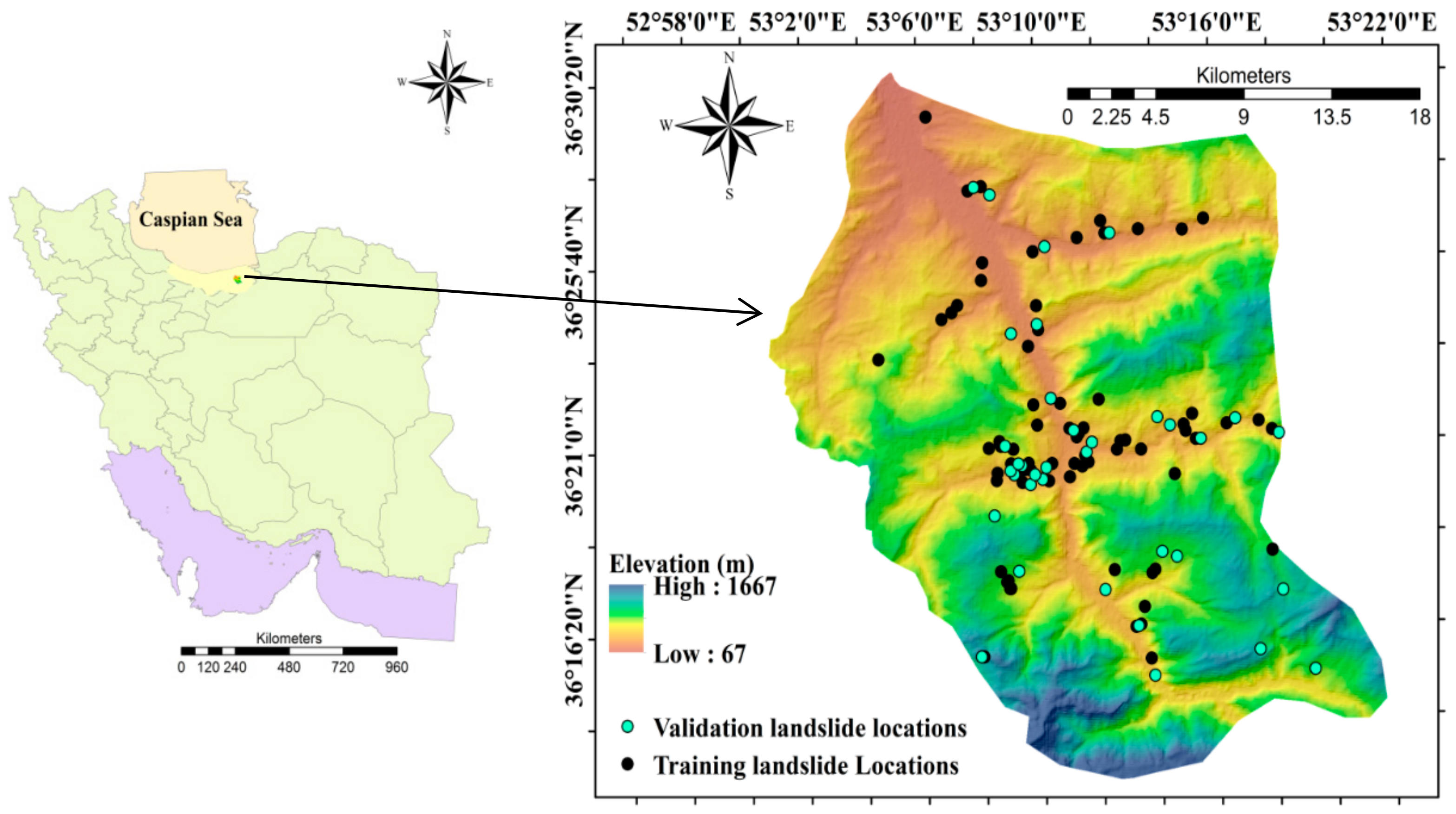
2. Materials and Methods

In this section, we describe the data collected and used and the background theory of the methods used for landslide susceptibility modeling. From these, the data including landslide susceptibility map and landslide conditioning factors were prepared and processed to generate the datasets for constructing and validating the models. The methods include bivariate models (FR, SE, WoE, and EBF) which were used for landslide susceptibility assessment, whereas validation methods (the ROC and AUC) were selected for validating the performance of the bivariate models.

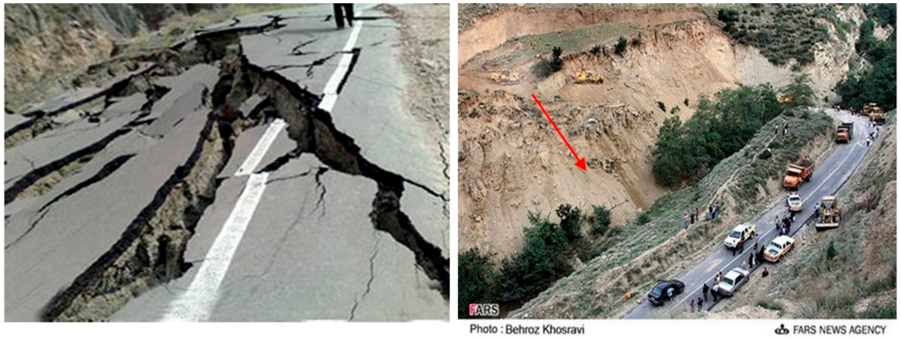
2.1. Landslide Inventory Mapping

The basic phase in LSM is building an inventory map based on the past landslide occurrences [24]. The accuracy of the data on past and present landslides is crucial in predicting future landslides [11,30]. In this research, for collecting the required data, extensive surveys in the field were conducted and aerial photographs were interpreted. A sum of 109 landslides were determined and mapped for preparing the landslide inventory map (Figure 1 and Figure 2). Chung and Fabbri [31] noted the impossibility of validating the functionality of a model without dividing the dataset. Accordingly, the inventory data was randomly categorized into two parts of 70% (74 locations) for building the model, which was called training dataset, and 30% (35 locations), which, not being used in the training step, was applied for validating the model performance, called the test dataset. The ratio of 70/30 for dividing the data for generating training and testing datasets was selected based on the suggestion of Pham et al. [16,30], Pradhan [19] and Pourghasemi et al. [24].

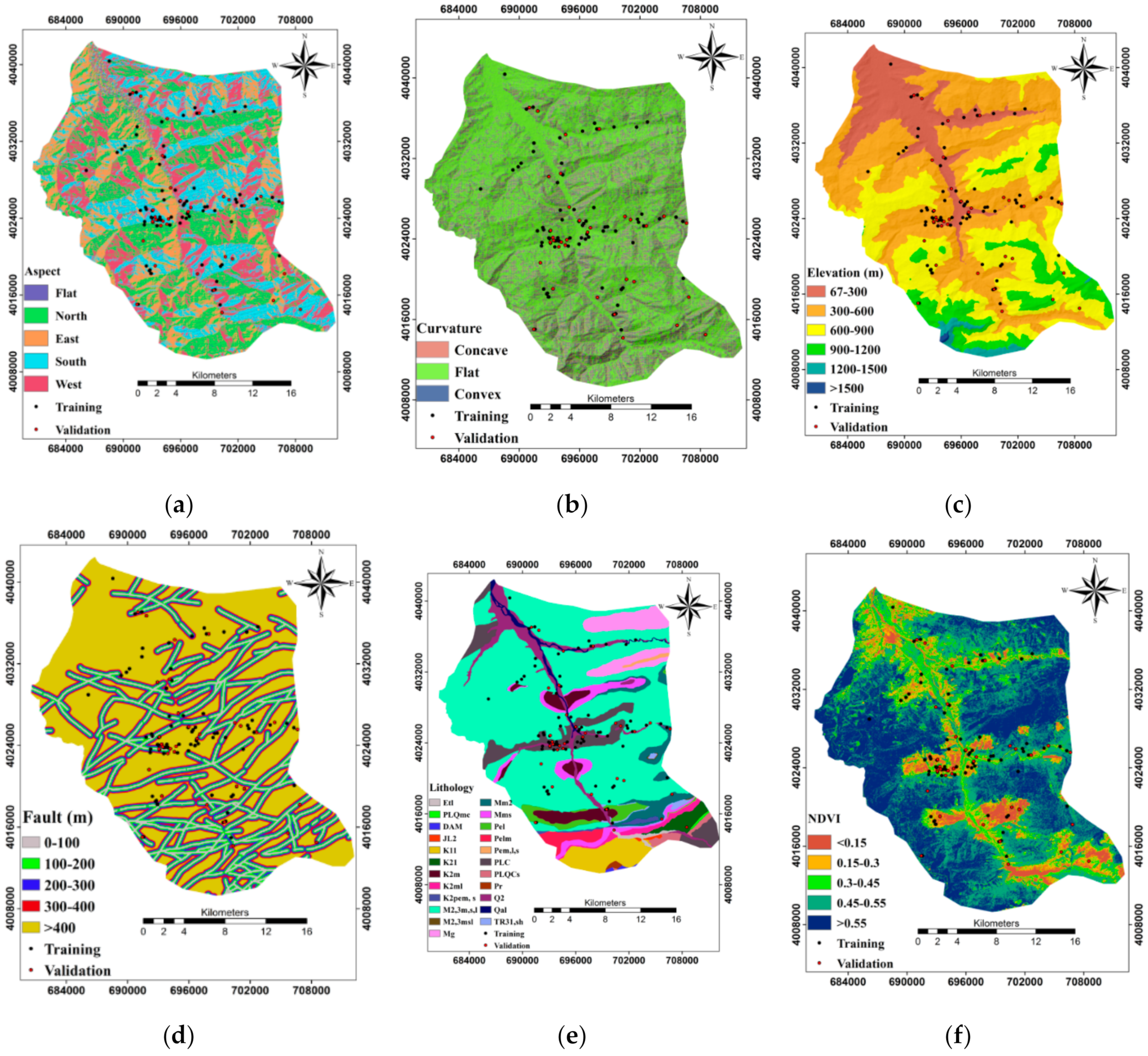
2.2. Landslide Conditioning Factors

To develop an assessment method for the assessment of susceptibility to landslides, identifying the landslide conditioning factors is crucial [32]. Landslide conditioning factors have some characteristics such as easy obtainability, representativeness, and practicality [21]. Ten conditioning factors affecting the occurrence of landslides were determined for LSM in this study based on the literature review and field surveys. The mechanism of landslide occurrence was identified to be related to hydrology, geomorphology, geology, etc. These factors were the slope aspect, curvature, elevation, distance from fault, lithology, normalized difference vegetation index (NDVI), distance from the river, distance from the road, the slope angle, and land use. In subsequent parts of the study, the first step is preparation of the digital elevation model (DEM). Using DEM of 30 × 30 m resolution (22,819 row and 9321 column), downloaded from ASTER global DEM, the slope angle, the slope aspect, elevation, and curvature were identified in ArcGIS 10.1 software.

2.2.1. Slope Aspect

The slope aspect is among the most significant factors affecting the occurrence of landslides due to various wetness of the aspect [33]. It affects hydrological processes because of evapotranspiration [34] and then, influences soil moisture and vegetation cover [35,36]. The information about the slope aspect was directly taken from DEM and divided into five categories, namely (1) flat, (2) north, (3) east, (4) south, and (5) west (Figure 3a).

2.2.2. Curvature

The morphology of the topography was identified by curvature [5]. This factor controls surface runoff and therefore, has an impact on landslide occurrence [37,38]. The curvature was straight drawn from the DEM and categorized into three classes of negative curvature, i.e., concave (<−0.05), zero curvature, i.e., flat (−0.05–0.05), and positive curvature, i.e., convex (>0.05) (Figure 3b).

2.2.3. Elevation

The influence of elevation is not direct on landslide occurrences, but it affects other parameters such as rainfall, tectonics, etc. [39,40]. Similarly, this factor was taken from the DEM and categorized in six groups based on the landslide frequency analysis: (1) 67–300; (2) 300–600; (3) 600–900; (4) 900–1200; (5) 1200–1500; and (6) >1500 (Figure 3c).

2.2.4. Distance from Fault

The fault leads to discontinuity of soil and rocks [41]. Generally, tectonic breaks reduce the rock strength and initiate many landslides [42]. The fault layer was derived from the fault map of Iran. Then, the distance from the fault was extracted using the multiple ring buffers command in ArcGIS10.1 with five classes of 0–100, 100–200, 200–300, 300–400, and >400 m, based on literature studies [41,42] (Figure 3d).

2.2.5. Lithology

The different formations have various structures, compositions, and permeability, which influence the formation material strength [43]. Therefore, the confluence of these factors with curvature and slope steepness has a remarkable influence on landslide occurrences [44]. The lithological feature was derived from the geological map of Mazandaran, which consisted of 22 units (Table 1 and Figure 3e).

2.2.6. NDVI

The NDVI map was generated through Landsat 7/ETM+ by ENVI 5 software (Figure 3f). The greater the NDVI value is, the more the amount of vegetation cover. The root of vegetation leads to stabilization of the hill slope and reduction in landslide occurrences.

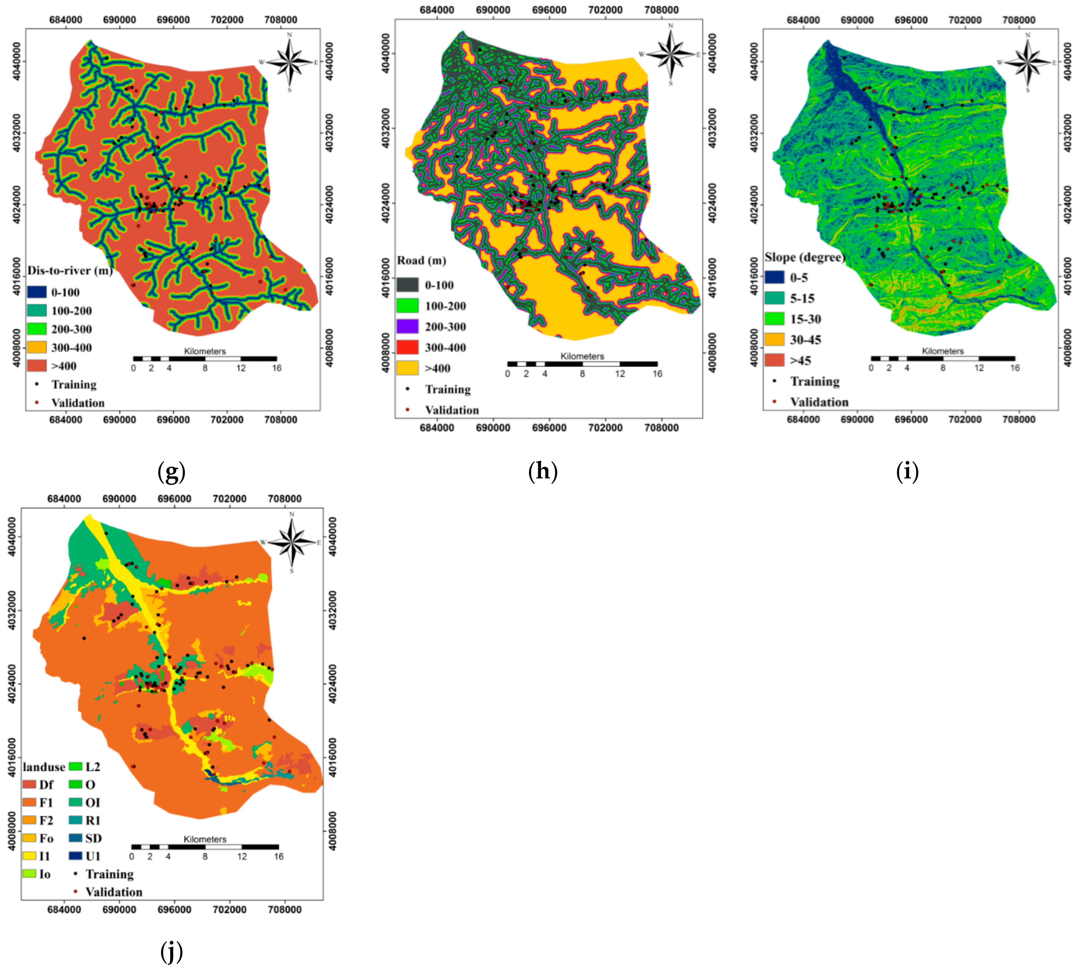
2.2.7. Distance from River

The water of the river is considered as one of the main sources of e soil moisture. Binh Thai et al. [45] in their research stated that 65.12% of landslides occurred in the first class of the distance from the river (0–40 m). Accordingly, it is a very important factor in LSM. This factor was extracted for the river layer through buffering and classified into five classes including (1) 0–100, (2) 100–200, (3) 200–300, (4) 300–400, and (5) >400 m (Figure 3g).

2.2.8. Distance from Road

Tuan and Dan [46] stated that landslides were mostly distributed near the road system. By cutting the slope hills for construction of roads in the slopes more than 10 degrees, discontinuity is made in the soil and rock. Accordingly, the area can be prone to landslides [41]. The distances to the roads were obtained and divided into six classes of (1) 0–100, (2) 100–200, (3) 200–300, (4) 300–400, and (5) >400 m (Figure 3h).

2.2.9. Slope Angle

The slope angle is among the most significant conditioning factors in the occurrence of landslides [8], because it is related to shear stress and contributes to the displacement of the hill slope [47,48,49]. Wherever the thickness of the soil is sufficient, by increasing the slope angle, the hill slope can be more unstable. The slope angles in the area under study were reclassified into five groups of (1) 0–5, (2) 5–15, (3) 15–30, (4) 30–45, and (5) >45 degrees (Figure 3i).

2.2.10. Land Use

Land use is a significant factor that affects the landslides in the area under study. The land-use map for Mazandaran province was extracted with the following types: Dry farming (DF), sparse forest (F1), semi-dense forest (F2), integrated forest and orchards (FO), irrigated farming (I1), integrated irrigated farming and orchards (IO), bare land (L2), orchards (O), integrated orchards and irrigated farming, sparse rangeland (R1), storage dams (SD), and residential area (U1) (Figure 3j). In the regions covered by vegetation, the vegetation roots play the role of anchors and lead to an increase in soil and rock mass stability [50].

2.3. Bivariate Models

2.3.1. Frequency Ratio (FR)

As Bonham-Carter [51] stated, FR represents the possibility of the occurrence for a given characteristic. The FR method is on the basis of the observed relationships between the distribution of landslide occurrence locations and each of the factors influencing landslides and is used to reveal the correlation between them [52]. Greater FR values than 1 indicate the great proportion of landslide occurrences to the area and a high correlation. Conversely, the smaller FR values than 1 show a weak correlation [53]. Equation (1) shows the FR algorithm used in this study [54]:
W i j = F L i j F N i j
where W i j shows the FR of class i of parameter j; F L i j is the frequency of occurrence of landslides for class i of parameter j; and F N i j is the frequency of non-occurrence of landslides for class i of parameter j.
To calculate and make the LSM, the FR values of parameters influencing landslides were added together [54]. Finally, the LSM was determined by adding the FR values of parameters together using Equation (2).
L S M = j = 1 n W i j
where W i j is the weight of class i of parameter j, and n is the number of conditioning factors.

2.3.2. Shannon Entropy (SE)

Entropy is the measure of abnormality, changeability, unstable behavior, and uncertainty in each system [6]. Generally, the entropy concept is described as the quantity of abnormality between causes and results or in determination on various topics [55]. The entropy index is an estimate of the difference between the average shares of single groups in the whole system [55]. The SE model benefits from an extremely close relationship between the quantity and entropy, called Boltzmann, which is utilized to show the thermodynamic conditions of a system [6]. The Shannon method is adjusted on the basis of the Boltzmann concept and the entropy model is utilized in information theory [6]. The following formulae are used in the calculation of the information coefficient and Vj represents the parameter value to total value ratio [56], determined the equation below:
E i j = F R j = 1 M j F R
where FR represents the value of the frequency ratio and E i j is the probability density for each class:
H j = i = 1 M j E i j log 2 E i j ,   j = 1 , , n
H j max = log 2 M j ,   M j n u m b e r   o f   c l a s s e s
I j = H j max H j / H j max ,   I = ( 0 , 1 ) ,   j = 1 ,
V j = I j F R
where H j and H j max are the values of entropy, I j is information coefficient, M j is number of classes in each conditioning factor, and V j is the achieved weight value for the given parameter. The range of variations is between zero and 1. The values close to 1 have higher inconsistency and imbalance [27].

2.3.3. Weights of Evidence (WoE)

Some binary patterns may be joined together to predict another binary pattern for the WoE model. Many benefits of the WoE model over other statistical methods, including being data-driven based on the Bayesian probabilistic method, have made it a fairly popular statistical method [19].
The two basic parameters, which are very crucial to running the model, are negative weight (W) and positive weight (W+) [19,27]. This method estimates the weight of each conditioning factor (A) on the basis of the presence or absence of occurrences (e.g., of landslide) within a specified area as in the following [51].
W + = l n P B | A P B | A
W = l n P B ¯ | A P B ¯ | A ¯
where P is probability and Ln is the natural logarithm. B and B ¯ are the presence or absence of landside conditioning factors, respectively. Further, A and A ¯ are the presence or absence of a landslide occurrence, respectively [26,57]. The variation of the parameter W+ from W is called weight contrast [58].
The amount of the weight contrast displays the spatial relationship between factors affecting the occurrence of a landslide. The standard deviation of positive and negative weights, S(c), is computed as follows:
S C = S 2 W + + S 2 W
where SW+ and SW are the variances of positive and negative weights, respectively. The variances of positive and negative weights can be estimated through the following equations:
S 2 W + = 1 N { B A } + 1 B A ¯
S 2 W = 1 { B ¯ A } + 1 B ¯ A ¯
The studentized contrast, i.e., the ratio of the contrast to its standard deviation, is used to calculate confidence:
W f i n a l = ( C / S ( C ) )

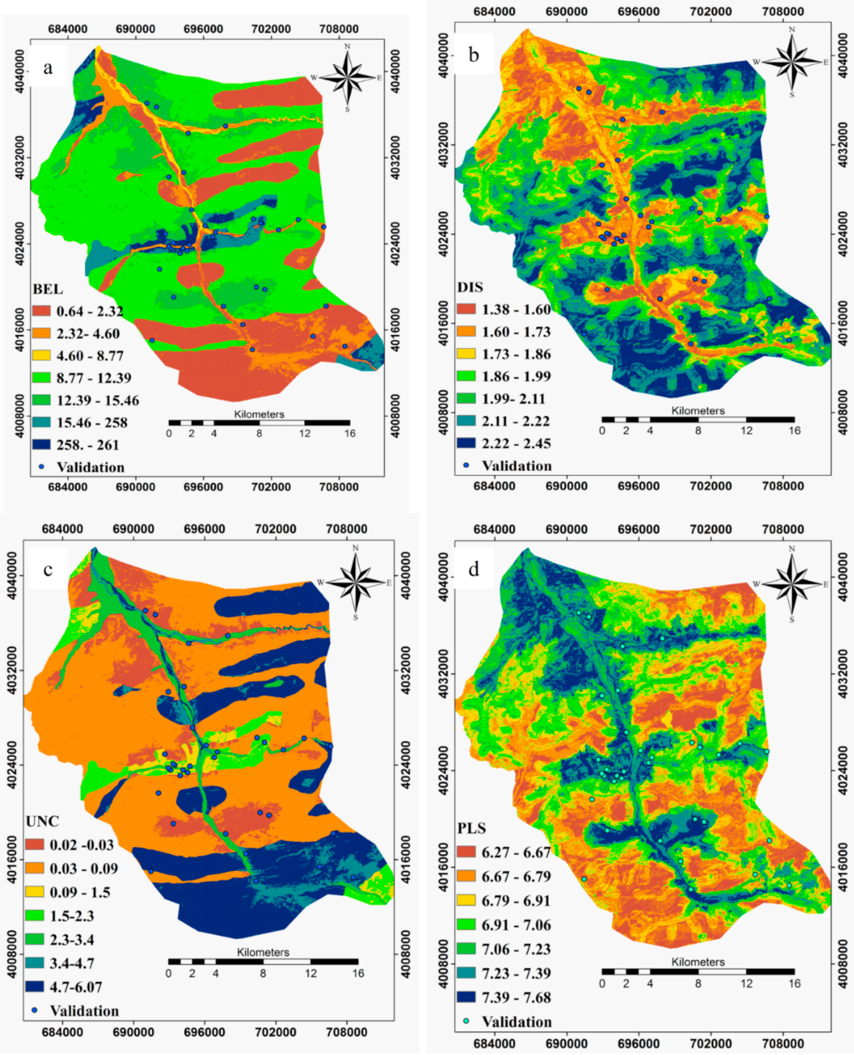
2.3.4. Evidential Belief Function (EBF)

The EBF model is fundamentally based on the theory of Dempster-Shafer of evidence [59]. The advantage of this model is that it presents predicted flood zones, landslide zones, etc. with uncertainty [60]. There are four basic parameters in EBF model, including degree of belief (Bel), degree of disbelief (Dis), degree of uncertainty (Unc), and degree of plausibility (Pls) [15,61].
It should be noted that suitable classification of all factors influencing landslides should have the same size of cells and appropriate time resolution. In this phase, L number of the input data layers can be considered as probability (Eij) in order to achieve correct results, in which (ij) represents i number of factors and j is the class characteristics. The total values of the EBF for factors affecting landslides were calculated one after the other by Equations (14) to (19). Equations (14) and (15) show how to achieve the results of Bel.
λ T p E i j = N / D = N L E i j / N L / [ N E i j N L E i j / N A   N L
B e l = λ Tp Eij / λ   T p E i j
where N L E i j represents the number of landslide pixels per class, N (L) stands for the sum of the occurrences of landslides, N (Eij) is pixels per class for each factor, N (A) denotes the sum of pixels in the area under study, N is the proportion of areas with landslide occurrences, and D represents the proportion of areas without landslides. These values are obtained by Equations (16) and (17).
λ T p ¯ E i j = K H = N L N L E i j / N L / [ N A N L N E i j + N L E i j / N A N L
D i s = λ T p ¯ Eij / λ T p ¯ E i j
where K is the rate of landslides not occurring and H is the rate of occurrences in non-landslide areas. Equations (18) and (19) were utilized for all classes of factors affecting landslides and then, Equations (13) and (15) were used to prepare the results for Bel and Dis. The values of Pls and Uuc were determined by the following equations.
Unc = 1 − Dis − Bel
Pls = 1 − Dis
The range of Bel and Pls values is between 0 and 1. The most important limitation of the EBF, according to the findings of Park [60], is that if there is no occurrence of landslide in a specific class, then Bel results are equal to zero. Dis is also be equal to zero and in this case, Unc or uncertainty values are equal to 1.

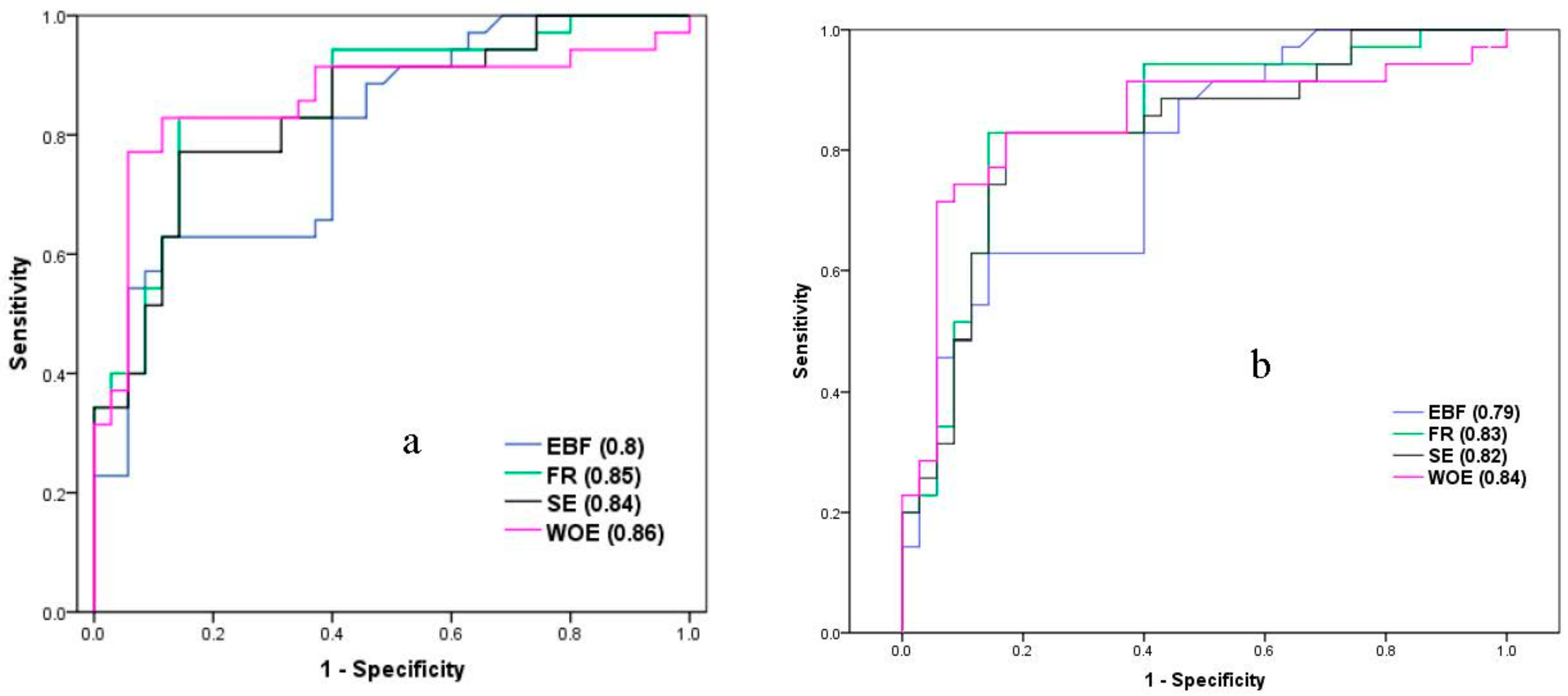
2.4. Model Verification

To verify the performance of LSM, in this study, the authors have used the receiver operating characteristic (ROC) curve and the area under the curve (AUC). ROC is one of the most popular methods [62,63] and it is a practical technique of showing the quality of deterministic and probabilistic detections [64] used to determine the accuracy of the LSMs [23]. The ROC curve was drawn by plotting specificity on the X axis and sensitivity on the Y axis. Sensitivity is the false positive rate and specificity is the false negative as presented below:
Sensitivity = TP/(TP + FN)
Specificity = TN/(FP + TN)
where true positive (TP) is the number of observed landslides predicted accurately and true negative (TN) is the total non-occurring landslides that have been predicted accurately. On the other hand, false positive (FP) is considered as the number of occurring landslides inaccurately categorized in the non-landslide classes and false negative (FN) is considered as the number of non-occurring landslides inaccurately categorized in the landslide classes.
The AUC can identify the model’s accuracy and ability in predicting future landslides. The range of the AUC ranges from 0.5 to 1 with the AUC of 1 representing perfect prediction and the closer the value of the AUC to this number, the better the performance of the model [58].

3. Results

3.1. Multicollinearity Diagnosis
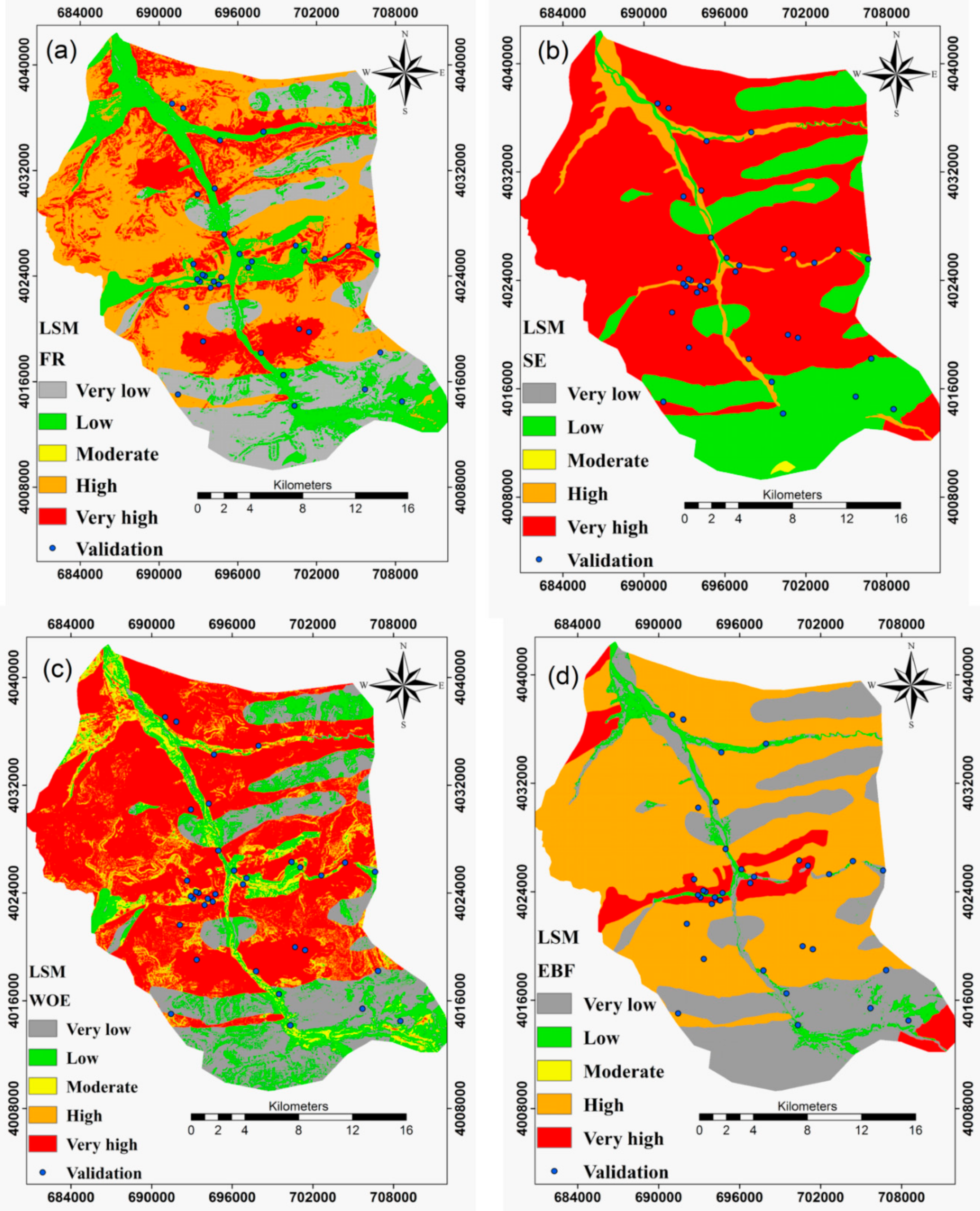
In this study, a multicollinearity test was conducted by variance inflation factors (VIF) and the tolerances method for selection of suitable landslide conditioning factors to identify whether there was correlation between the conditioning factors (Table 2). The values of VIF > 10 or tolerance < 0.1 show a problem of multicollinearity in conditioning factors [6]. According to the multicollinearity test results (Table 2), no collinearity was observed among the 10 conditioning factors affecting the landslide.

3.2. FR Model

The results of the FR method showed the weights obtained for each of the classes of factors. As represented in Table 3, the FR was calculated for 10 factors based on their relationships with landslide occurrences. The ratio of the area with landslide occurrences to the whole area was identified. The higher the value of the FR is, the stronger the correlation of the factors with landslide occurrences. The greater values of the FR than 1 show a strong correlation and those below 1 show a weak correlation [65].
The results showed that among the geographical directions, north weighing 1.57 had the most significant impact on the landslide occurrences in Klijanrestagh Watershed in Mazandaran province. The lowest weight was for the flat areas where no landslide had occurred.
Regarding the conditioning factor of curvature, convex curvature with the value of 1.1 had the greatest impact and concave and flat curvatures respectively weighing 0.86 and 0.98 had very small impact on the landslides in the area under study. The other important factor that may affect landslide is elevation. The lowest elevation (67–300 m) had the greatest impact on the landslide (1.58) followed by the second class (300–600), which had a weight of 1.47. Other elevation classes had a low impact on landslides. To study the influence of regional faults on landslides, the impact of different distances from the fault on landslides was calculated and the outcomes revealed that the first class (distance of 0 to 100 m) weighing 1.33 had the highest impact on landslide occurrences in the area under study. The units of PLQCs, Qal, and TR31, sh with the respective weights of 30, 14, and 4 had a high impact on landslides in the area under study.
The lowest NDVI value had the highest impact on landslides. Another factor affecting landslides is the distance from the river. In the results, the first 4 classes (from 0 to 400 m) had positive effects on landslides and the effects were smaller for classes of more than 400 m. Among various distances in the road network, the first class (0–100 m) weighing 1.8 had the greatest impact on landslides and then was the second class (100–200 m) with a weight of 1.3. The analysis of the FR method showed that the third class (15–30) and second slope (5–15) with FR values of 1.16 and 1.03 exerted the greatest effect on landslides occurring in the area under study.
Regarding land use, the garden with the weight of 8.3 and dry farming with the weight of 3.4 had the most significant effects on landslide occurrences. Equation (22) was used in GIS and finally, LSM was prepared using the FR model.
L S M F R = F R S l o p e + F R C u r v a t u r e + F R D i s R i v e r + F R e l e v a t i o n + F R L a n d u s e + F R D i s R o a d l + F R D i s f a u l t I + F R a s p e c t + F R L i t h o log y + F R N D V I

3.3. SE Model

The results of SE for the relationship of the effective factors with the occurrence of landslides are presented in Table 3. Lithology factors, elevation classes, land use, and NDVI respectively weighing 40.7, 1.8, 0.62, and 0.57 are the most important factors affecting landslides in Klijanrestagh Watershed. Other factors in order of importance and the effects on landslides are aspect, slope, distance from the road, distance from the river, distance from the faults, and terrestrial curvature weighing 0.14, 0.11, 0.09, 0.06, 0.03, and 0.005, respectively. Using Equation (23), the LSM was prepared using the SE model.
L S M S E = 0.14 * A s p e c t F R + 0.005 * c u r v a t u r e FR + 1.804 * e l e v a t i o n FR + 0.35 * f a u l t FR + 40.7 * l i t o FR + 0.57 * N D V I FR + 0.065 * D i s River FR + 0.094 * D i s r o a d + 0.112 * S l o p e   FR + 0.62 * L U L C FR

3.4. WoE Model

Like the FR model, this model is utilized to attain the weights of factors affecting landslides and the relationship of landslide occurrences with the related classes. The results of this model in this study are shown in Table 3. The WoE model is based on W+ and W. W+ indicates that predictable variables are present in landslide locations and its magnitude represents the effect magnitude of the condition factors on landslides [66]. W indicates the absence of conditioning factors in landslide occurrences and indicates a negative correlation between factors and the occurrence of landslides [3]. Therefore, C for the positive spatial association is positive and for the negative spatial association is negative.
S2W+ and S2W are variances of W + and W, respectively. S(C) is the standard deviation of contrast and C/S(C) is studentized values of contrast (Table 3). C/S(C) is the final weight of the WoE method. The map of effective weighted factors was prepared by assigning this weight to each factor. Finally, the LSM was produced implementing the following equation.
L S M W O f E = A s p e c t W O f E + c u r v a t u r e W O f E + e l e v a t i o n W O f E + f a u l t W O f E + l i t j o W O f E + N D V I W O f E + D i s river W O f E + D i s r o a d W O f E + S l o p e W O f E + L U L C W O f E
Considering the values of C/S(C) in Table 3 for the aspect, the northern class of the aspect had the most significant effect (3.05) on landslides. Other classes, having negative weights, showed no significant correlation with the occurrence of landslides. The results showed that the convex curvature had a significant positive effect (0.47) and concave and flat curvatures had negative effects on landslides. Like in the FR method, the first 2 classes of the elevation conditioning factor had the largest impact and the rest had lower effects on landslide occurrences. The elevation of 300–600 m weighing 3.39 had the greatest effect on landslides. Class 0–100 m of the distance from the fault weighing 1.13 exerted the most remarkable effect on landslides, and classes 100–200 and 200–300 m had the lowest effects on landslides in the area under study.
Regarding the lithology factor, the M2msl unit weighing 32 had the highest impact on landslide occurrences. Another effective factor affecting landslides was NDVI. The lowest NDVI values had the highest impact on landslides Therefore, the landslide occurrence probability was reduced with the increase in the NDVI value. The risk of landslides decreased with the distance from the river, because moisture, as a major cause of landslide occurrences, decreased. The first class of the distance from the river (100–200 m) weighing 2.61 had the greatest effect on landslides. As with the distance from the river, the risk of landslides was reduced with the distance from the road. In this study, the first class of the distance from the road (0–100 m) with a weight of 4 had the greatest effect on landslides. The probability of the occurrence of landslides increased with the slope up to 30 degrees and then, decreased. The highest effect on landslides was related to the slope class of 15–30 degrees. Based on this method, dry farming had the greatest effect on landslides, while the FR method introduced garden use for the greatest effect. After dry farming weighing 5.3, the combination of garden and dry farming weighing 5.1, and garden weighing 3 as well as the forest with the average density had the highest effects on landslides, respectively.

3.5. EBF Model

The EBF method was utilized to explore the relationship between locations of the occurring landslides and the landslide conditioning factors. The results depicted the weight of each class of factors in landslides (Table 3).
In the map of the aspect, the northern direction with 44% events had the highest probability of the occurrence of landslides weighting 0.39, as it was less exposed to sunlight and had higher moisture than other directions. The results of the curvature map analysis showed that the convex curvature had the greatest impact on landslides.
As in the FR method, the first class of elevation weighing 4 had the greatest effect on landslides in this method. Class 0–100 m of the distance from the fault had the greatest effect on landslides as 19% of landslide events were observed in this distance, which consisted in only 14% of the basin area. In the case of the lithology factor, the M2,3msl and PLQC units weighing 256 and 7, respectively, had the greatest effects on the occurrence of landslides in Klijanrestagh Basin.
Another factor that would affect landslides and was considered in this study was NDVI. The lowest NDVI value, which was less than 0.15 and weighed 1.2, had the highest impact on the occurrence of landslides. The results of the distance from the river and locations of the occurring landslides showed that the risk of landslides decreased with the distance from the river. Therefore, the second class (100–200) and first class (0–100 m) had the highest effect on landslides occurring in the study area.
The landslide risk decreased with the increase in the distance from the road. The first class (0–100 m) had the greatest effect (BEL = 0.45) on landslides. Considering the slope factor, the slope of 15–30 degrees with BEL of 0.29 had the greatest effect and the slopes more than 45% (BEL = 0) had the lowest effect on landslides. The highest weights were for garden (BEL = 2.1) and forest (BEL = 1.4).
Figure 4 presents the EBF results. The map of bel (Figure 4a) shows the distribution of landslides. A comparison was drawn between belief and disbelief maps (Figure 4b), and the results showed that areas with higher bel values had lower dis and vice versa, that is, the areas more prone to landslides were those with higher degrees of belief and lower degrees of disbelief about the occurrence of landslides. According to Unc map, areas with the highest sensitivity to landslides had the minimum values of Unc. Pls map is almost similar to bel and represents great values for areas with high belief values and low uncertainty. The results comply well with Carranza and Hale [61], Bui et al. [67] and Nampak et al. [68].
Finally, the LSM was utilized through the relationships provided above for the FR, SE, WoE, and EBF models and then, four maps were prepared based on the quantile method, which is one of the most popular classification methods [26], which are shown in Figure 5.

3.6. Assessment and Comparison of the Models

In this research study, the well-known ROC and area under the curve (AUC) techniques were applied.to assess and compare the models There are two main steps in model evaluation by AUC, namely, the success rate evaluation and the prediction rate evaluation. The results for the success rate were achieved on the basis of training data and the prediction rates were attained by a set of validation data. The results of the success rate represented the fitness of the model for the training data and because the training points on which the model was built were used in the success rate. The success rate method was not useful in assessing the predicting power of the model [68].
The area under the curve of the success rate for the FR, SE, WoE, and EBF models was 0.85, 0.84, 0.86, and 0.8, respectively (Figure 6a). Further, the area under the curve of the prediction rate for the FR, SE, WoE, and EBF models was 0.83, 0.82, 0.84, and 0.79, respectively (Figure 6b). The AUC amount of 0.84 for the WoE shows 84% prediction accuracy of the model. Considering the results of the evaluation by the AUC, the most accurate prediction in the identification of LSM is for the WoE model and the least accurate prediction is for the EBF. However, generally, prediction accuracies of these four models are reasonable.

4. Discussion

The preparation of landslide susceptibility is one of the most practical approaches for landslide hazard assessment and proper management tasks [69]. Although, there are many models developed for the LSM, there is no a universal guideline for model selection to model better LSMs. In this study, the four most popular and widely used state-of-the art statistical bivariate models (i.e., FR, SE, WOE and EBF) were applied for the LSM in Klijanrestagh Watershed, Iran.
Modeling results mostly depend on both the model’s structure and quality of data [70]. The most effective data were selected and their quality was investigated through a multicollinearity test and the SE model. The results of these two tests showed that all applied conditioning factors are effective and independent. According to the SE model, the aspect, the slope and the distance from the road were the most effective factors and curvature was the least effective factor on landslide occurrences. This result is in accordance with the results of other research reports [70,71,72,73,74,75]. The improper road construction in the study area can be revealed as the one of the most effective criteria on landslide occurrences.
The results showed that the north aspect had the highest effect on landside occurrences, and the main reason may be that the north aspect has the most wetness among other aspects resulting from less solar radiation [70]. Regarding the curvature, convex has the most effect on landslide occurrences, especially when combined with improper road construction that cause failure slopes. The risk of landslides decreased with the elevation in the area under study as the depth of soil reduced sharply. The results show that there is a linear relationship between landslide occurrences and faults, as faults are a disconnection in the earth and thus, can cause landslides more easily. The lowest NDVI value had the highest impact on landslides. This is because a higher NDVI value means higher vegetation cover, which can help to prevent landslides. The distances of 100 to 200 m from the river and road exerted the greatest impact on landslides occurring in the area under study since the closer to the river the higher the wetness, therefore, the higher the landslide occurrences probability. These findings are consistent with results of other literature studies [75,76,77]. These results are approximately consistent among the FR, WoE and EBF models.
This study showed that WOE has the highest prediction power, followed by FR, SE and EBF, respectively. According to Park [60], the main limitation of the EBF method is that if a landslide event does not happen in a given class, the Bel results will be equal to zero. In addition, when the Unc or uncertainty values are equal to 1, Dis will be zero. But EBF model despite its lower capability for prediction of landslide-prone areas benefited from belief, disbelief, plausibility, and uncertainty maps, which were very practical. Thus, it can be concluded that the results of the predictions about the landslide-prone areas by modeling the uncertainty degree (Unc) show the relationships between landslide occurrences and multiple spatial data layers quantitatively [60]. The power of prediction of the FR was highly identical to that of SE method, which complies well with Youssef et al. [17].
In general, WOE model was found the best model in this study for identification of landslide-prone areas as this data-driven method has some advantages, which may lead to its high accuracy in comparison with other methods. They are (i) WoE model benefits from the Bayesian-based theorem in a log-linear form using prior and posterior probabilities and (ii) WoE model is effectively utilized when sufficient dataset is in hand for predicting the relative significance of evidential themes using statistical tools.

5. Conclusions

Landslide susceptibility modeling for the future is one of the vital and difficult tasks in the assessment of the risk of landslides. Many methods have been proposed for spatial prediction of natural hazards including landslides, e.g., bivariate statistical, multivariate statistical, data mining, etc. However, the accuracy of the predictions of these models is still under debate as their accuracy varies from one watershed to another. Kelijanrestagh Watershed in Mazandaran province, Iran, is a hot spot of landslide occurrences with many landslides occurring in each year. In this research, four models, namely FR, SE, WoE, and EBF, were utilized in landslide susceptibility mapping of Kelijanrestagh Watershed in Mazandaran province, Iran.
A total of 109 locations of landslides were determined by extensive surveys in the field and mapped in a landslide inventory map. The locations were categorized into two main datasets for training and validation. In the next step, 10 landslide conditioning factors were selected by a review of the literature and on the basis of the characteristics of the area under study and availability of data. Finally, the LSMs were prepared and mapped with five classes (very low, low, moderate, high and very high) using four models.
Next, the four produced maps were evaluated using training and testing datasets and ROC and AUC (success rate and prediction rate) methods. The AUC results indicated the success rates of 0.8, 0.86, 0.84, and 0.85 for EBF, WoE, SE, and FR, respectively. Further, they presented the prediction rates of 0.84, 0.83, 0.82, and 0.79 for WoE, FR, SE, and EBF models, respectively. Therefore, the WoE model, having the greatest AUC, was the most accurate method among the four implemented methods in identifying areas at risk of future landslides in the area under study.
The outcomes of this research can be helpful for decision makers and future development planners to avoid the zones with high susceptibility during implementing a project. However, it is recommended that a comparative study needs to be conducted (i.e., comparison between data mining algorithms, data intelligence, statistical bivariate models, multivariate models, multi criteria decision making models) applied for solving this challenge of which model should be applied, which precision and accuracy is reasonable, and so on. The field survey is a difficult approach for the preparation of the landslide inventory map, especially for elevation which often affects landslide distribution. Landslides that occur in high altitude areas are often lost, because of the difficulty of accurate field surveys. Thus, it is recommended that identification of landslide locations should be based on high-resolution satellite images.

Author Contributions

E.N., M.S. and S.S. collected the data, K.K. and B.T.P. performed modeling and analysis. E.N., M.S., S.S., K.K. and B.T.P. wrote the manuscript. B.P., S.L. and A.M.M. provided critical comments in planning this paper and edited the manuscript. All the authors discussed the results and edited the manuscript.

Funding

This research was conducted by the Basic Research Project of the Korea Institute of Geoscience and Mineral Resources (KIGAM) funded by the Ministry of Science and ICT.

Conflicts of Interest

The authors declare no conflict of interest.

References

  1. Chakraborty, S.; Pradhan, R. Development of GIS based landslide information system for the region of East Sikkim. Int. J. Comput. Appl. 2012, 49, 5–9. [Google Scholar] [CrossRef]
  2. Goetz, J.N.; Guthrie, R.H.; Brenning, A. Integrating physical and empirical landslide susceptibility models using generalized additive models. Geomorphology 2011, 129, 376–386. [Google Scholar] [CrossRef]
  3. Regmi, A.D.; Devkota, K.C.; Yoshida, K.; Pradhan, B.; Pourghasemi, H.R.; Kumamoto, T.; Akgun, A. Application of frequency ratio, statistical index, and weights-of-evidence models and their comparison in landslide susceptibility mapping in Central Nepal Himalaya. Arab. J. Geosci. 2014, 7, 725–742. [Google Scholar] [CrossRef]
  4. Trigila, A.; Iadanza, C.; Esposito, C.; Scarascia-Mugnozza, G. Comparison of Logistic Regression and Random Forests techniques for shallow landslide susceptibility assessment in Giampilieri (NE Sicily, Italy). Geomorphology 2015, 249, 119–136. [Google Scholar] [CrossRef]
  5. Pourghasemi, H.; Moradi, H.; Aghda, S.F. Landslide susceptibility mapping by binary logistic regression, analytical hierarchy process, and statistical index models and assessment of their performances. Nat. Hazards 2013, 69, 749–779. [Google Scholar] [CrossRef]
  6. Pourghasemi, H.R.; Mohammady, M.; Pradhan, B. Landslide susceptibility mapping using index of entropy and conditional probability models in GIS: Safarood Basin, Iran. Catena 2012, 97, 71–84. [Google Scholar] [CrossRef]
  7. Kanungo, D.; Arora, M.; Sarkar, S.; Gupta, R. Landslide Susceptibility Zonation (LSZ) Mapping—A Review. J. South Asia Disaster Stud. 2009, 2, 81–105. [Google Scholar]
  8. Van Den Eeckhaut, M.; Vanwalleghem, T.; Poesen, J.; Govers, G.; Verstraeten, G.; Vandekerckhove, L. Prediction of landslide susceptibility using rare events logistic regression: A case-study in the Flemish Ardennes (Belgium). Geomorphology 2006, 76, 392–410. [Google Scholar] [CrossRef]
  9. Monsieurs, E.; Dewitte, O.; Demoulin, A. A susceptibility-based rainfall threshold approach for landslide occurrence. Nat. Hazard Earth Syst. Sci. 2019, 19, 775–789. [Google Scholar] [CrossRef] [Green Version]
  10. Holec, J.; Bednarik, M.; Šabo, M.; Minár, J.; Yilmaz, I.; Marschalko, M. A small-scale landslide susceptibility assessment for the territory of Western Carpathians. Nat. Hazards 2013, 69, 1081–1107. [Google Scholar] [CrossRef]
  11. Reichenbach, P.; Rossi, M.; Malamud, B.; Mihri, M.; Guzzetti, F. A review of statistically-based landslide susceptibility models. Earth Sci. Rev. 2018, 180, 60–91. [Google Scholar] [CrossRef]
  12. Dahal, R.K.; Hasegawa, S.; Nonomura, A.; Yamanaka, M.; Masuda, T.; Nishino, K. GIS-based weights-of-evidence modelling of rainfall-induced landslides in small catchments for landslide susceptibility mapping. Environ. Geol. 2008, 54, 311–324. [Google Scholar] [CrossRef]
  13. Hjort, J.; Luoto, M. 2.6 Statistical Methods for Geomorphic Distribution Modeling. In Treatise on Geomorphology; Academic Press: San Diego, CA, USA, 2013; pp. 59–73. [Google Scholar]
  14. Tsangaratos, P.; Ilia, I.; Rozos, D. Case Event System for Landslide Susceptibility Analysis. In Landslide Science and Practice; Springer: Berlin/Heidelberg, Germany, 2013; pp. 585–593. [Google Scholar]
  15. Althuwaynee, O.F.; Pradhan, B.; Lee, S. Application of an evidential belief function model in landslide susceptibility mapping. Comput. Geosci. 2012, 44, 120–135. [Google Scholar] [CrossRef]
  16. Pham, B.T.; Tien Bui, D.; Indra, P.; Dholakia, M. Landslide susceptibility assessment at a part of Uttarakhand Himalaya, India using GIS–based statistical approach of frequency ratio method. Int. J. Eng. Res. Technol. 2015, 4, 338–344. [Google Scholar]
  17. Youssef, A.M.; Pradhan, B.; Jebur, M.N.; El-Harbi, H.M. Landslide susceptibility mapping using ensemble bivariate and multivariate statistical models in Fayfa area, Saudi Arabia. Environ. Earth Sci. 2015, 73, 3745–3761. [Google Scholar] [CrossRef]
  18. Lee, S.; Ryu, J.-H.; Lee, M.-J.; Won, J.-S. Use of an artificial neural network for analysis of the susceptibility to landslides at Boun, Korea. Environ. Geol. 2003, 44, 820–833. [Google Scholar] [CrossRef]
  19. Pradhan, B. Landslide susceptibility mapping of a catchment area using frequency ratio, fuzzy logic and multivariate logistic regression approaches. J. Indian Soc. Remote Sens. 2010, 38, 301–320. [Google Scholar] [CrossRef]
  20. Yilmaz, I. Comparison of landslide susceptibility mapping methodologies for Koyulhisar, Turkey: Conditional probability, logistic regression, artificial neural networks, and support vector machine. Environ. Earth Sci. 2010, 61, 821–836. [Google Scholar] [CrossRef]
  21. Oh, H.-J.; Pradhan, B. Application of a neuro-fuzzy model to landslide-susceptibility mapping for shallow landslides in a tropical hilly area. Comput. Geosci. 2011, 37, 1264–1276. [Google Scholar] [CrossRef]
  22. Sezer, E.A.; Pradhan, B.; Gokceoglu, C. Manifestation of an adaptive neuro-fuzzy model on landslide susceptibility mapping: Klang valley, Malaysia. Expert Syst. Appl. 2011, 38, 8208–8219. [Google Scholar] [CrossRef]
  23. Akgun, A.; Kıncal, C.; Pradhan, B. Application of remote sensing data and GIS for landslide risk assessment as an environmental threat to Izmir city (west Turkey). Environ. Monit. Assess. 2012, 184, 5453–5470. [Google Scholar] [CrossRef] [PubMed]
  24. Pourghasemi, H.R.; Pradhan, B.; Gokceoglu, C. Application of fuzzy logic and analytical hierarchy process (AHP) to landslide susceptibility mapping at Haraz watershed, Iran. Nat. Hazards 2102, 63, 965–996. [Google Scholar] [CrossRef]
  25. Althuwaynee, O.F.; Pradhan, B.; Park, H.-J.; Lee, J.H. A novel ensemble bivariate statistical evidential belief function with knowledge-based analytical hierarchy process and multivariate statistical logistic regression for landslide susceptibility mapping. Catena 2014, 114, 21–36. [Google Scholar] [CrossRef]
  26. Khosravi, K.; Nohani, E.; Maroufinia, E.; Pourghasemi, H.R. A GIS-based flood susceptibility assessment and its mapping in Iran: A comparison between frequency ratio and weights-of-evidence bivariate statistical models with multi-criteria decision-making technique. Nat. Hazards 2016, 83, 947–987. [Google Scholar] [CrossRef]
  27. Khosravi, K.; Pourghasemi, H.R.; Chapi, K.; Bahri, M. Flash flood susceptibility analysis and its mapping using different bivariate models in Iran: A comparison between Shannon’s entropy, statistical index, and weighting factor models. Environ. Monit. Assess. 2016, 188, 656. [Google Scholar] [CrossRef] [PubMed]
  28. Zhang, G.; Cai, Y.; Zheng, Z.; Zhen, J.; Liu, Y.; Huang, K. Integration of the statistical index method and the analytic hierarchy process technique for the assessment of landslide susceptibility in Huizhou, China. Catena 2016, 142, 233–244. [Google Scholar] [CrossRef]
  29. Pourghasemi, H.R.; Kerle, N. Random forests and evidential belief function-based landslide susceptibility assessment in Western Mazandaran Province, Iran. Environ. Earth Sci. 2016, 75, 185. [Google Scholar] [CrossRef]
  30. Thai Pham, B.; Bui, D.T.; Prakash, I. Landslide susceptibility modelling using different advanced decision trees methods. Civ. Eng. Environ. Syst. 2018, 35, 139–157. [Google Scholar] [CrossRef]
  31. Chung, C.-J.F.; Fabbri, A.G. Validation of spatial prediction models for landslide hazard mapping. Nat. Hazards 2003, 30, 451–472. [Google Scholar] [CrossRef]
  32. Ercanoglu, M.; Gokceoglu, C. Assessment of landslide susceptibility for a landslide-prone area (north of Yenice, NW Turkey) by fuzzy approach. Environ. Geol. 2002, 41, 720–730. [Google Scholar]
  33. Sadr, M.P.; Maghsoudi, A.; Saljoughi, B.S. Landslide susceptibility mapping of Komroud sub-basin using fuzzy logic approach. Geodyn. Res. Int. Bull. 2014, 2, XVI–XXVIII. [Google Scholar]
  34. Sidle, R.C.; Ochiai, H. Landslides: Processes, Prediction, and Land Use; Water Resources Monograph Series; American Geophysical Union: Washington, DC, USA, 2006. [Google Scholar]
  35. Jaafari, A.; Panahi, M.; Pham, B.T.; Shahabi, H.; Bui, D.T.; Rezaie, F.; Lee, S. Meta optimization of an adaptive neuro-fuzzy inference system with grey wolf optimizer and biogeography-based optimization algorithms for spatial prediction of landslide susceptibility. Catena 2019, 175, 430–445. [Google Scholar] [CrossRef]
  36. Qingfeng, H.; Zhihao, X.; Shaojun, L.; Renwei, L.; Shuai, Z.; Nianqin, W.; Pham, B.T.; Wei, C. Novel Entropy and Rotation Forest-Based Credal Decision Tree Classifier for Landslide Susceptibility Modeling. Entropy 2019, 21(2), 106. [Google Scholar] [Green Version]
  37. Dou, J.; Yunus, A.P.; Bui, D.T.; Merghadi, A.; Sahana, M.; Zhu, Z.; Chen, C.W.; Khosravi, K.; Yang, Y.; Pham, B.T. Assessment of advanced random forest and decision tree algorithms for modeling rainfall-induced landslide susceptibility in the Izu-Oshima Volcanic Island, Japan. Sci. Total Environ. 2019, 662, 332–346. [Google Scholar] [CrossRef] [PubMed]
  38. Pham, B.T.; Prakash, I.; Khosravi, K.; Chapi, K.; Trinh, P.T.; Nog, T.Q.; Hossini, S.V.; Bui, D.T. A comparison of Support Vector Machines and Bayesian algorithms for landslide susceptibility modelling. Geocarto Int. 2018. [Google Scholar] [CrossRef]
  39. Shirzadi, A.; Soliamani, K.; Habibnejhad, M.; Kavian, A.; Chapi, K.; Shahabi, H.; Chen, W.; Khosravi, K.; Thai Pham, B.; Pradhan, B.; et al. Novel GIS based machine learning algorithms for shallow landslide susceptibility mapping. Sensors 2018, 18, 3777. [Google Scholar] [CrossRef]
  40. Thai Pham, B.; Prakash, I.; Dou, J.; Singh, S.K.; Trinh, P.T.; Tran, H.T.; Le, T.M.; Phong, T.V.; Khoi, D.K.; Shirzadi, A.; et al. A Novel Hybrid Approach of Landslide Susceptibility Modeling Using Rotation Forest Ensemble and Different Base Classifiers. Geocarto Int. 2018, 1–38. [Google Scholar]
  41. Ayalew, L.; Yamagishi, H. The application of GIS-based logistic regression for landslide susceptibility mapping in the Kakuda-Yahiko Mountains, Central Japan. Geomorphology 2005, 65, 15–31. [Google Scholar] [CrossRef]
  42. Devkota, K.C.; Regmi, A.D.; Pourghasemi, H.R.; Yishida, K.; Pradhan, B.; Ryu, I.C.; Dhital, M.R.; Althuwaynee, O.F. Landslide susceptibility mapping using certainty factor, index of entropy and logistic regression models in GIS and their comparison at Mugling–Narayanghat road section in Nepal Himalaya. Nat. Hazards 2013, 65, 135–165. [Google Scholar] [CrossRef]
  43. Hong, H.; Naghibi, S.A.; Pourghasemi, H.R.; Pradhan, B. GIS-based landslide spatial modeling in Ganzhou City, China. Arab. J. Geosci. 2016, 9, 112. [Google Scholar] [CrossRef]
  44. Nguyen, V.V.; Pham, B.T.; Vv, B.T.; Prakash, I.; Jha, S.; Shahabi, H.; Shirzadi, A.; Ba, D.N.; Kumar, R.; Chatterjee, J.M.; et al. Hybrid Machine Learning Approaches for Landslide Susceptibility Modeling. Forests 2019, 10, 157. [Google Scholar] [CrossRef]
  45. Binh Thai, P.; Dieu, T.B.; Indra, P. Application of Classification and Regression Trees for Spatial Prediction of Rainfall Induced Shallow Landslides in the Uttarakhand Area (India) Using GIS. In Climate Change, Extreme Events and Disaster Risk Reduction; Springer: Berlin/Heidelberg, Germany, 2017; pp. 159–170. [Google Scholar]
  46. Tuan, T.; Dan, N. Landslide susceptibility mapping and zoning in the Son La hydropower catchment area using the analytical hierarchy process. J. Sci. Earth 2012, 3, 223–232. [Google Scholar]
  47. Fayez , L.; Thai Pham, B.; Solanki, H.A.; Pazhman, D.; Dholakia, M.B.; Khalid, M.; Prakash, I. Application of Frequency Ratio Model for the Development of Landslide Susceptibility Mapping at Part of Uttarakhand State, India. Int. J. Appl. Eng. Res. 2018, 13, 6846–6854. [Google Scholar]
  48. Pham, B.T. A Novel Classifier Based on Composite Hyper-cubes on Iterated Random Projections for Assessment of Landslide Susceptibility. J. Geol. Soc. India 2018, 91, 355–362. [Google Scholar] [CrossRef]
  49. Pham, B.T.; Prakash, I.; Jaafari, A.; Bui, D.T. Spatial prediction of rainfall-induced landslides using aggregating one-dependence estimators classifier. J. Indian Soc. Remote Sens. 2018, 46, 1457–1470. [Google Scholar] [CrossRef]
  50. Salvatici, T.; Tofani, V.; Rossi, G.; D’Ambrosio, M.; Tacconi Stefanelli, C.; Benedetta Masi, E.; Rosi, A.; Pazzi, V.; Vannocci, P.; Petrolo, M.; et al. Application of a physically based model to forecast shallow. Nat. Hazards Earth Syst. Sci. 2018, 18, 1919–1935. [Google Scholar] [CrossRef]
  51. Bonham-Carter, G.F. Geographic Information Systems for Geoscientists: Modelling with GIS vol 13; Elsevier: Amsterdam, The Netherlands, 2014. [Google Scholar]
  52. Lee, S.; Talib, J.A. Probabilistic landslide susceptibility and factor effect analysis. Environ. Geol. 2005, 47, 982–990. [Google Scholar] [CrossRef]
  53. Akgun, A.; Dag, S.; Bulut, F. Landslide susceptibility mapping for a landslide-prone area (Findikli, NE of Turkey) by likelihood-frequency ratio and weighted linear combination models. Environ. Geol. 2008, 54, 1127–1143. [Google Scholar] [CrossRef]
  54. Youssef, A.M.; Pradhan, B.; Pourghasemi, H.R.; Abdullahi, S. Landslide susceptibility assessment at Wadi Jawrah Basin, Jizan region, Saudi Arabia using two bivariate models in GIS. Geosci. J. 2015, 19, 449–469. [Google Scholar] [CrossRef]
  55. Wan, S. A spatial decision support system for extracting the core factors and thresholds for landslide susceptibility map. Eng. Geol. 2009, 108, 237–251. [Google Scholar] [CrossRef]
  56. Bednarik, M.; Magulová, B.; Matys, M.; Marschalko, M. Landslide susceptibility assessment of the Kraľovany–Liptovský Mikuláš railway case study. Phys. Chem. Earth Parts A/B/C 2010, 35, 162–171. [Google Scholar] [CrossRef]
  57. Xu, C.; Xu, X.; Lee, Y.H.; Tan, X.; Yu, G.; Dai, F. The 2010 Yushu earthquake triggered landslide hazard mapping using GIS and weight of evidence modeling. Environ. Earth Sci. 2012, 66, 1603–1616. [Google Scholar] [CrossRef]
  58. Tehrany, M.S.; Pradhan, B.; Jebur, M.N. Spatial prediction of flood susceptible areas using rule based decision tree (DT) and a novel ensemble bivariate and multivariate statistical models in GIS. J. Hydrol. 2013, 504, 69–79. [Google Scholar] [CrossRef]
  59. Dempster, A.P. Upper and Lower Probabilities Induced by a Multivalued Mapping. In Classic Works of the Dempster-Shafer Theory of Belief Functions; Springer: Berlin/Heidelberg, Germany, 2008; pp. 57–72. [Google Scholar]
  60. Park, N.-W. Application of Dempster-Shafer theory of evidence to GIS-based landslide susceptibility analysis. Environ. Earth Sci. 2011, 62, 367–376. [Google Scholar] [CrossRef]
  61. Carranza, E.J.M.; Hale, M. Evidential belief functions for data-driven geologically constrained mapping of gold potential, Baguio district, Philippines. Ore Geol. Rev. 2003, 22, 117–132. [Google Scholar] [CrossRef]
  62. Jaafari, A.; Zenner, E.K.; Pham, B.T. Wildfire spatial pattern analysis in the Zagros Mountains, Iran: A comparative study of decision tree based classifiers. Ecol. Inform. 2018, 43, 200–211. [Google Scholar] [CrossRef]
  63. Tien Bui, D.; Shahabi, H.; Shiezadi, A.; Chapi, K.; Honang, N.-D.; Pham, B.T.; Bui, Q.-T.; Tran, C.-T.; Panahi, M.; Bin Ahmad, B.; et al. A novel integrated approach of relevance vector machine optimized by imperialist competitive algorithm for spatial modeling of shallow landslides. Remote Sens. 2018, 10, 1538. [Google Scholar] [CrossRef]
  64. Swets, J.A. Measuring the accuracy of diagnostic systems. Science 1988, 240, 1285–1293. [Google Scholar] [CrossRef]
  65. Pradhan, B. Manifestation of an advanced fuzzy logic model coupled with Geo-information techniques to landslide susceptibility mapping and their comparison with logistic regression modelling. Environ. Ecol. Stat. 2011, 18, 471–493. [Google Scholar] [CrossRef]
  66. Pradhan, B.; Oh, H.; Buchroithner, M. Weights-of-evidence model applied to landslide susceptibility mapping in a tropical hilly area. Geomat. Nat. Hazards Risk 2010, 1, 199–223. [Google Scholar] [CrossRef]
  67. Bui, D.T.; Pradhan, B.; Lofman, O.; Revhaug, I.; Dick, O.B. Spatial prediction of landslide hazards in Hoa Binh province (Vietnam): A comparative assessment of the efficacy of evidential belief functions and fuzzy logic models. Catena 2012, 96, 28–40. [Google Scholar]
  68. Nampak, H.; Pradhan, B.; Manap, M.A. Application of GIS based data driven evidential belief function model to predict groundwater potential zonation. J. Hydrol. 2014, 513, 283–300. [Google Scholar] [CrossRef]
  69. Guzzetti, F. Landslide Hazard and Risk Assessment. Ph.D. Thesis, University of Bonn, Bonn, Germany, 2006. [Google Scholar]
  70. Pham, B.T.; Khosravi, K.; Prakhsh, I. Application and comparison of decision tree-based machine learning methods in landside susceptibility assessment at Pauri Garhwal Area, Uttarakhand, India. Environ. Process. 2017, 4, 711–730. [Google Scholar] [CrossRef]
  71. Chen, W.; Zhao, X.; Shahabi, H.; Shirzadi, A.; Khosravi, K.; Chai, H.; Zhang, S.; Zhang, L.; Ma, J.; Chen, Y.; et al. Spatial prediction of landslide susceptibility by combining evidential belief function, logistic regression and logistic model tree. Geocarto Int. 2019. [Google Scholar] [CrossRef]
  72. Gholami, M.; Ghachkanlu, E.; Khosravi, K.; Pirasteh, S. Landslide prediction capability by comparison of frequency ratio, fuzzy gamma and landslide index method. J. Earth Syst. Sci. 2019, 128, 42. [Google Scholar] [CrossRef] [Green Version]
  73. Tien Bui, D.; Shahabi, H.; Omidvar, E.; Shirzadi, A.; Geertsema, A.; Clague, J.; Khosravi, K.; Pradhan, B.; Pham, B.; Chapi, K.; et al. Shallow landslide prediction using a novel hybrid functional machine learning algorithm. Remote Sens. 2019, 11, 931. [Google Scholar] [CrossRef]
  74. Chen, W.; Shahabi, H.; Zhang, S.; Khosravi, K.; Shirzadi, A.; Chapi, K.; Pham, B.T.; Zhang, T.; Zhang, L.; Chai, H.; et al. Landslide susceptibility modeling based on gis and novel bagging-based kernel logistic regression. Appl. Sci. 2018, 8, 2540. [Google Scholar] [CrossRef]
  75. Hung, P.V.; Son, P.Q.; Dung, N.V. The study evaluated arming of risk of landslide in Hoa Binh and Son La reservoir hydropower area on the basis of analyzing high-resolution remote sensing and geographic information systems. Vietnam J. Earth Sci. 2015, 37, 193–203. [Google Scholar]
  76. Tan, M.T.; Tao, N.V. Studying landslides in Thua Thien—Hue province. Vietnam J. Earth Sci. 2014, 36, 121–130. [Google Scholar] [CrossRef]
  77. Thom, B.V.; Son, P.Q.; Hung, P.V.; Anh, N.T.V. Research assessment landslide and sedimentation of Hoa Binh hydropower reservoir. Vietnam J. Earth Sci. 2016, 38, 131–142. [Google Scholar]
Figure 1. Landslide location map of the study area.
Water 11 01402 g001
Figure 2. Some photos of landslides occurring in the area under study.
Water 11 01402 g002
Figure 3. (a) Slope aspect, (b) curvature, (c) elevation, (d) distance from the fault, (e) lithology, (f) NDVI, (g) distance from the river, (h) distance from the road, (i) the slope angle, and (j) land use.
Water 11 01402 g003aWater 11 01402 g003b
Figure 4. The combined results of the EBF model: (a) belief, (b) disbelief, (c) uncertainty, and (d) plausibility.
Water 11 01402 g004
Figure 5. Landslide susceptibility maps produced by (a) FR, (b) SE, (c) WoE, and (d) EBF models.
Water 11 01402 g005
Figure 6. Model validation for Klijanrestagh Watershed: (a) success rate curve and (b) prediction rate curve.
Water 11 01402 g006
Table 1. Lithological description of the study area.
NoCodeLithology
1Et.lAndesitic volcanic tuff
2PLQmcConglomerate, Sandston, siltstone, Silty Marl
3JL2Lime
4K11Hyporite bearing limestone (Senonian)
5K2lThick-bedded to massive limestone (maastrichtian)
6K2mLime and Quinasine
7lMarl, shale and detritic limestone
8K2PemsMarl, shale, limestone and mixture of conglomerate
9M23m,s,lMarl, calcareous sandstone, sandy limestone and minor conglomerate
10M2mslMarl and calcareous sandstone
11MgRed conglomerate and sandstone
12Mm2Marl and calcareous
13MmsMarl, calcareous sandstone and sandy limestone
14PelMedium to thick-bedded limestone
15PelmMedium to thick-bedded limestone
16PemlsDark grey medium-bedded to massive limestone
17PlcPolymictic conglomerate and sandstone
18PLQcsConglomerate, Sandston and siltstone
19PrFusulina limestone, dolomitic limestone
20Q2New Alluvial
21QalLoose alluvium in the river channels
22TR3l,shShale, Lime and Dolomite
Table 2. Indices of multicollinearity diagnosis for landslide conditioning factors.
ModelCollinearity Statistics
ToleranceVIF
Slope aspect0.3532.833
Curvature0.3003.331
Altitude (m)0.8061.240
Distance from fault0.7741.293
NDVI0.3323.016
Lithology0.7841.275
Distance from river (m)0.7141.401
Distance from road (m)0.8761.142
Slope angle (degree)
Land use0.3772.656
Table 3. The correlation between occurring landslides and each conditioning factor using bivariate models.
Landslide NumberPercent of LandslideNumber of PixelsPercent of PixelsFRSEWoEBELDISUNCPLS
Factors
Aspect
Flat00.00326252.040.000.14None0.000.200.7950.79
North3344.0044816228.051.573.010.390.150.4480.84
East1216.0034606321.660.74−1.180.180.210.5980.78
South1418.6738720924.240.77−1.120.190.210.5900.78
West1621.3338339924.000.89−0.540.220.200.5680.79
Curvature
Concave810.6719899112.460.860.005−0.470.210.200.5790.79
Flat5168.00109186668.350.98−0.070.250.200.5460.79
Convex1621.3330660119.191.110.470.280.190.5240.80
Elevation
67–3001824.0024193515.141.581.8042.110.400.180.4210.82
300–6004762.6768282242.741.473.390.370.130.4990.86
600–900912.0049034930.700.39−3.320.090.250.6460.74
900–120011.331563849.790.14−2.070.030.220.7460.78
1200–150000.00241151.510.00None0.000.200.7960.79
>150000.0018530.120.00None0.000.200.7990.79
Distance to Fault
0–1001418.6722501414.091.330.0351.130.330.190.4760.81
100–20045.3321246313.300.40−1.950.100.210.6800.78
200–300810.6719058611.930.89−0.340.220.2040.5710.79
300–40079.3316557310.370.90−0.290.220.2030.5700.79
>4004256.0080373350.321.110.980.280.1780.5420.82
Lithology
Etl00.0075870.470.0040.7None0.000.2020.7980.79
PLQmc00.0015860.100.00None0.000.2010.7990.79
DAM00.0016200.100.00None0.000.2010.7990.79
JL200.0021130.130.00None0.000.2010.7990.79
K1100.00619223.880.00None0.000.2090.7910.79
K2100.00215911.350.00None0.000.2040.7960.79
K2m00.00488973.060.00None0.000.2070.7930.79
K2ml00.00179791.130.00None0.000.2030.7970.79
K2pem, s00.0082570.520.00None0.000.2020.7980.79
M2,3m, s, l00.0093529958.550.00None0.000.4840.5160.51
M2,3msl3952.008570.05969.232.752560.096−2550.90
Mg00.00767904.810.00None0.000.2110.7890.78
Mm211.33570063.570.37−1.000.090.2050.7000.79
Mms22.67612713.840.70−0.520.170.2030.6210.79
Pel00.00302841.900.00None0.000.2050.7950.79
Pelm11.33216131.350.99−0.010.240.2010.5510.79
Pem,l,s00.0046550.290.00None0.0000.2010.7990.79
PLC00.001094906.850.00None0.000.2160.7840.78
PLQCs1722.67117660.7430.7713.337.770.156−6.9270.84
Pr00.0024450.150.00None0.000.2010.7990.79
Q211.33853425.340.50−1.420.060.2090.7280.79
Qal1317.33191381.2014.479.343.650.168−2.8180.83
TR31, sh11.3399090.624.300.770.540.1990.2590.80
NDVI
<0.152432.001047806.564.880.577.691.230.146−0.3760.85
0.15–0.32229.331166347.304.026.551.010.153−0.1660.84
0.3–0.451013.3321008713.151.010.050.250.2000.5440.80
0.45–0.551317.3354343134.020.51−2.950.120.2520.6200.74
>0.5568.0062251538.970.21−4.680.050.3030.6460.69
Distance to River
0–1001317.331571339.841.760.062.140.440.1840.3720.81
100–2001520.0016823410.531.902.610.470.1800.3420.82
200–300912.0018269911.441.050.150.260.2000.5360.80
300–4001520.0019679412.321.622.000.400.1830.4070.81
>4002330.6789250955.870.55−4.200.130.3150.5460.68
Distance to Road
0–1003648.0042235526.441.820.114.080.450.1420.4000.85
100–2001824.0029113418.231.321.290.330.1870.4810.81
200–30068.0021076213.190.61−1.310.150.2130.6340.78
300–400810.671551349.711.100.280.270.1990.5240.80
>40079.3351798432.430.29−3.880.070.2690.6580.73
Slope (degree)
0–579.3323130414.480.640.11−1.250.160.2130.6250.78
5–153952.0080415350.341.030.290.260.1940.5450.80
15–302634.6747781629.911.160.900.290.1870.5210.81
30–4534.00782864.900.82−0.360.200.2030.5910.79
>4500.0058990.370.00None0.000.2020.7980.79
Land use
Df1824.001118687.003.430.625.300.860.164−0.0280.83
F12533.33111551969.820.48−6.250.120.4440.4360.55
F211.3337470.235.691.741.430.199−0.6320.80
Fo34.00652274.080.98−0.040.240.2010.5520.79
I145.331110536.950.77−0.550.190.2040.6020.79
Io11.33230161.440.93−0.080.230.2010.5660.79
L200.002380.010.00None0.000.2010.7990.79
O22.6750880.328.373.002.110.196−1.3080.80
OI2128.001506909.432.975.120.740.1600.0920.84
R100.0071970.450.00None0.000.2020.7980.79
SD00.0030460.190.00None0.000.2010.7990.79
U100.0010150.060.00None0.000.2010.7990.79

