Numerical Simulation and Experiment Study on the Characteristics of Non-Darcian Flow and Rheological Consolidation of Saturated Clay

Abstract

To investigate the characteristics of the non-Darcian water flow through saturated clay and one-dimensional rheological consolidation behaviors of the soil in the Henan Province, we conducted constant-head permeability and one-dimensional rheological consolidation tests with one-way drainage using improved permeameter and oedometer tests, respectively. We then used Hansbo’s flow equation to classify the permeability test results and one-dimensional rheological consolidation equation combined with unified hardening (UH) constitutive model considering time effect was introduced to simulate the oedometer test results. The obtained results showed that the improved constant-head permeability test device was suitable for saturated clays, and that the UH constitutive model and Hansbo’s flow equation had good applications for the saturated clays investigated in this experiment.

1. Introduction

Terzaghi’s [1] one-dimensional consolidation theory has been widely employed by researchers since its introduction. Especially in areas with saturated clay, researchers have found that settlement values predicted by Terzaghi’s theory have large deviations from measured values, mainly because this theory ignores the influence of non-Darcian flow of pore water seepage and the rheological properties of saturated clays. Therefore, many researchers have conducted studies on saturated clays considering the above two factors. As early as 1898, King [2] found a deviation from Darcy flow in saturated clays, which was unfortunately unrecognized by the academic community at the time. In 1960, Hansbo [3] also witnessed this phenomenon, which he called the non-Darcian flow, and proposed a corresponding mathematical model using experimental results. The non-Darcian flow phenomenon in saturated clays was subsequently confirmed by many researchers around the world, and different mathematical equations were proposed for it. For example, Swartzendruber [4] proposed the non-Newtonian index flow model, Slepicka [5] proposed the exponential flow model, Miller et al. [6] proposed the threshold gradient flow model, and Qi et al. [7] proposed the broken line flow model. At the same time, Dubin et al. [8], Wang et al. [9], Deng et al. [10], Sun et al. [11], performed experiments showing that seepage in the relevant clays deviated from Darcy’s law in varying degrees. Wang et al. [9] attributed the deviation to the combined action of gravity water, capillary water, and weak bound water in saturated clay under different hydraulic gradients. Currently, Hansbo’s [3] flow theory is most commonly used, and has been applied to one-dimensional [12,13,14,15] and two-dimensional [16] consolidations, as well as sand drains [17], further confirming the necessity of considering non-Darcian flow in the analysis of saturated clay consolidation.

All these previous studies related to clay consolidation mostly focused on non-linearity [18,19], anisotropy [20], large-strain [21], time-dependent loading [22], and so on, while relatively few studies are related to the rheological properties of clay. Early studies [23,24,25] believe that the rheological properties of clay are caused by the viscosity of water around soil particles, the plastic adjustment of soil particles’ structure, the retention and creep due to shear stress, and hydrostatic pressure. However, there was a disagreement as to whether rheology should be taken into account during consolidation. Buisman [23] believed that rheological or secondary consolidation occurred after completing the main consolidation, while Tayor et al. [24] suggested that secondary consolidation occurred throughout the consolidation process. Bjerrum [26] confirmed Tayor’s theory through experiments and described the creep deformation of soil using a simple element model. Then, with continuous improvement in research methods, researchers around the world carried out in-depth research on the rheological properties of saturated clay based on one-dimensional rheological consolidation tests considering the effects of external load, loading ratio, preloading, drainage conditions, etc. First, Bjerrum [27] believed that the secondary consolidation coefficient was linearly related to the external load. However, Nash et al. [28] and Chen et al. [29] showed that the secondary consolidation coefficient first increased and then decreased with the increase in external load. Yin et al. [30] and Reddy et al. [31] further confirmed the above conclusion. Unlike Nash et al. [28], Chen et al. [29], Yin et al. [30], and Reddy et al. [31], it was found that the peak value of the secondary consolidation coefficient did not necessarily appear near pre-consolidation pressure, which Yin et al. [30] attributed to the effect of loading ratio and preloading. More in depth research ultimately demonstrated a high degree of nonlinearity in the deformation of saturated clay. Yin [32,33], Yao [34,35], and others have proposed some elastic visco-plastic (EVP) models. The unified hardening (UH) constitutive model was applied in one-dimensional rheological consolidation analysis, and successfully explained the increase in excess pore pressure near impervious surfaces at the initial stage of rheological consolidation. Compared to the EVP model proposed by Yin [32], the UH model proposed by Yao [34] has many advantages, such as fewer model parameters and a clearer physical concept, and thus could be simply determined by routine experiments.

In summary, in order to further explore the permeability and rheological consolidation characteristics of saturated clay, traditional permeability and one-dimensional consolidation test devices, as well as saturated remolded clay were improved based on previous works. A series of permeability and rheological consolidation tests were carried out, and their results were compared with fitting results obtained from Hansbo’s flow model and theoretical prediction results from the UH rheological consolidation model in order to verify the applicability of both models to saturated clay.

2. Experimental Study on the Permeability Characteristics of Saturated Clay

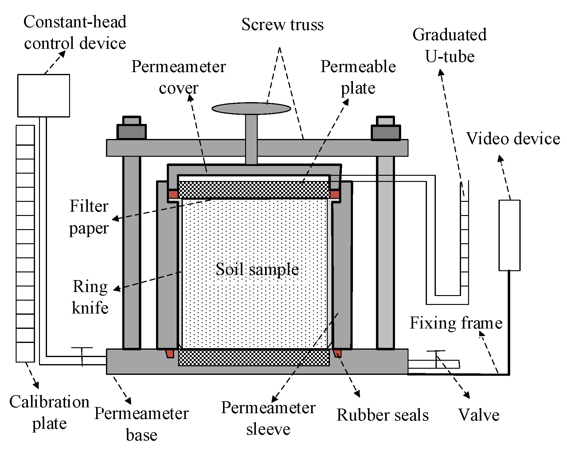
2.1. Constant-Head Permeability Test Device

Currently, there are two main types of permeability test methods, namely constant-head and falling-head [36]. Previous studies on saturated clay permeability employ the falling-head tests, but as shown in Figure 1, because of the compactness and low permeability of clay, the falling-head permeability test requires a long time, and the errors caused by human and environmental factors cannot be avoided during the test. However, it is noteworthy that the constant-head permeability test requires a very short time, but this test is primarily used to measure sand or granular soil with better permeabilities, and mostly to determine water volume using measuring cylinder or beaker. For clays with insignificant amounts of water flow and low permeability, it is impossible to measure water volume cannot be accurately measured in a short time; therefore, we improved the conventional constant-head permeability test device.

Figure 2 shows a schematic diagram of the improved constant-head test device proposed in this paper. Its main difference from the conventional constant-head permeability device is that in the modified device, a graduated U-tube with a 4 mm inner diameter was equipped with a video device to achieve accurate measurement of insignificant amounts of water flow in a short period of time. On the other hand, test head measurement was realized by combining the constant-head control device and calibration plate, which reduces test time and test error, and greatly improves test efficiency.

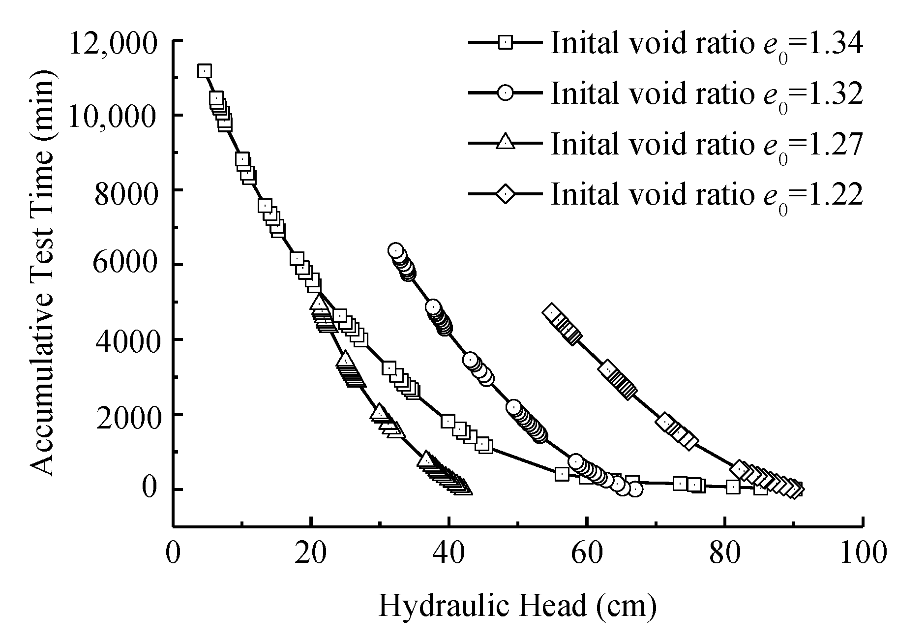
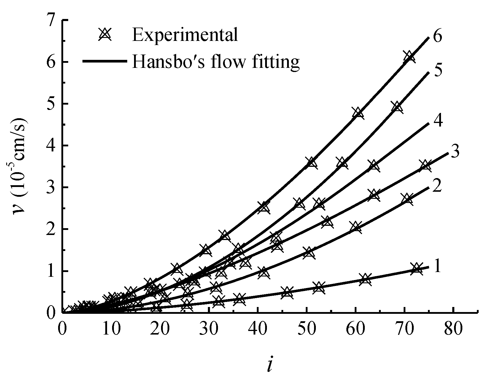
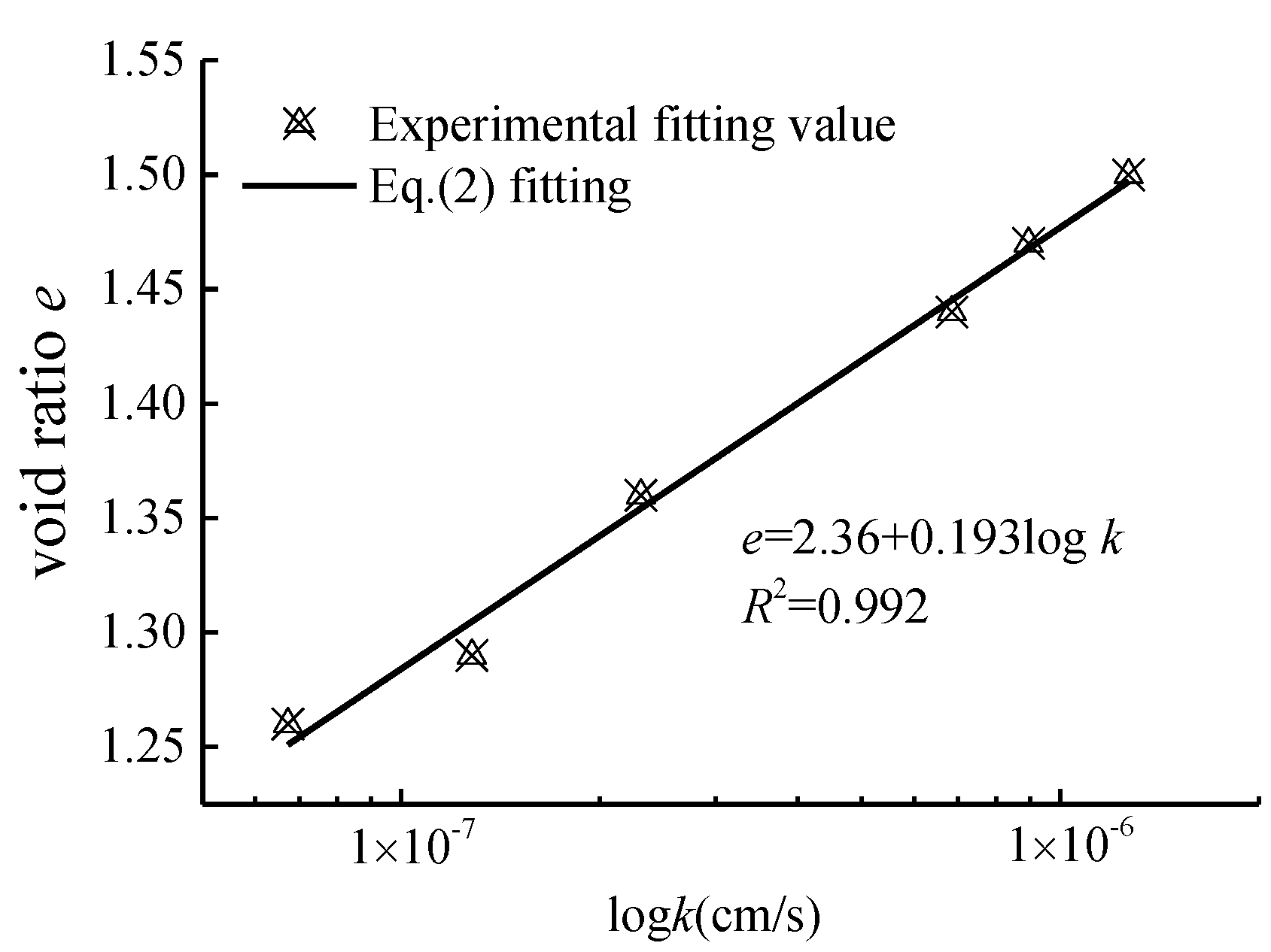
2.2. Permeability Test and Data Processing

The clay sample used in this paper was collected from a certain place in the Henan Province, at a 2.5 m depth. The basic physical parameters of the soil are summarized in

Table 1. Physical properties of soils.

Specific Gravity, Gs	Liquid Limit, wL (%)	Plastic Limit, wP (%)	Plastic Index, IP (%)
2.71	39.4	22.3	17.1

. Since natural undisturbed soil contains more impurities and it was not uniform, saturated remolded clay was used in this paper.

First, six permeability samples with different void ratios were prepared using a self-made saturated remolded clay sampler [37], according to the Standard for Soil Test Method (GB/T50123-1999) [36]. The height and diameter of the sample were 4 and 6.18 cm, respectively, and they were labeled SL-1 to SL-6. After vacuum saturation, permeability tests were carried out using the device described in Figure 2. The details of the test procedures were as follows: (1) Coat a layer of Vaseline on the inner wall of the permeameter sleeve, and attach a filter paper to the upper and lower surfaces of the saturated sample with cutting ring (to avoid being covered by Vaseline when the sample was installed, which could affect the permeability of the sample). Then, the sample was loaded into the permeameter sleeve, the excess Vaseline was wiped out and upper and lower filter papers were removed. Finally, permeameter sleeve was installed on the base and tighten the screw was tightened. (2) Constant head control device was adjusted and excess air inside the permeameter was discharged. Then, liquid levels were adjusted to calibration lines in the graduated U-tubes. (3) The left valve on the bottom of the permeameter was opened and the video device on the right side was turned on. it was left until liquid level in the U-tube reached the next calibration line and the test was stopped(where one scale was 0.034 mL, therefore the test time was shorter). Then, the constant head control device was adjusted using the same method and the corresponding seepage velocities under different constant pressure heads were recorded. Finally, v–i curves were obtained by connecting these experimental points.

Using the nonlinear fitting toolbox in Origin software and Hansbo’s [3] flow mathematical equations shown in Equation (1), permeability test data were segmentally fitted as shown in Figure 3. Test results were compared with those obtained from Hansbo’s flow fitting. The basic parameters of soil sample and Hansbo’s flow are summarized in

Table 2. Hansbo’s flow fitting parameters.

Soil Sample Number	e0	k (cm/s)	i0	m	R2
SL-1	1.26	6.73 × 10−8	22.20	1.45	0.985
SL-2	1.29	1.28 × 10−7	23.54	1.58	0.978
SL-3	1.36	2.31 × 10−7	27.81	1.63	0.964
SL-4	1.44	6.85 × 10−7	31.25	1.81	0.972
SL-5	1.47	8.95 × 10−7	24.37	1.64	0.967
SL-6	1.50	1.29 × 10−6	30.41	1.83	0.956

where e₀ is the initial void ratio , k is the permeability coefficient of soil samples, R² is the correlation coefficient.

.

$$v=\{\begin{array}{cc}c{i}^m,\hfill & i<i_1\hfill \\ k\left(i-i_0\right),\hfill & i\ge i_1\hfill \end{array}$$

(1)

where i₀ = i₁(m − 1)/m, c = k/(mi₁^m−1); c and k are the coefficient of permeability of the exponential flow at low gradients and the linear flow at high gradients, respectively; m is the exponent of exponential flow at low gradients; i₀ is the initial the hydraulic gradient of the linear percolation section; and i₁ is the threshold hydraulic gradient for the linear relationship. When i₀ = 0 or m = l, Equation (1) degenerates into Darcy’s flow law.

The developed fitting method was as follows: (1) If there were n experimental points, first Origin software was used for non-linearly fitting of 0 to g (where 0 < g < n) experimental points based on v = ci^m to obtain the values of c and m. (2) Equation $v=cm{i}_1^{m-1}\left[i-i_1\left(m-1\right)/m\right]$ was obtained by substituting c and m into formula $v=k\left(i-i_0\right)$, then the g to n experimental points were non-linearly fitted through equation $v=cm{i}_1^{m-1}\left[i-i_1\left(m-1\right)/m\right]$ by Origin software, and the value of i₁ was obtained. (3) By substituting the values of c, m, and i₁ into the Equation (1), the calculation points of Hansbo’s flow mathematical model were obtained, and the correlation between experimental and the calculation values was compared to obtain maximum R². Otherwise, the above methods were repeated at 0 to g + 1 and g + 1 to n experimental points. where e₀ is the initial void ratio, k is the permeability coefficient of soil samples, R² is the correlation coefficient.

Figure 3 and

Table 3. Basic properties of the rheological consolidation test sample.

Sample Number	Specific Gravity, Gs	Bulk Density, ρ (g/cm3)	Water Content, w (%)	Void Ratio, e0
LB-1	2.71	1.738	47.77	1.30
LB-2	2.71	1.864	34.14	0.95

show that the results obtained from Hansbo’s flow equation fitting and test results had a high degree of fitting with a correlation coefficient R² above 0.95. Hansbo’s flow parameter m was also within the ranges suggested by Hansbo [3], Dubin et al. [8], and Sun et al. [11] (between 1 and 2). However, due to the lack of relevant experimental data, there is no unified statement on the range of i₀ in current studies, Hansbo [3] stated that i₀ ranged from 1 to 4; Dubin et al. [8] reported it was between 3 and 25, and Sun et al. [11] reported it to be between 0.5 and 14, and the results obtained in this paper were basically within the above range, which proves the applicability of Hansbo’s flow model to clay samples.

Taylor [38] proposed a linear relationship between the logarithm of k and void ratio e as shown in Equation (2):

$$\log k=\log k_0-\left(e_0-e\right)/C_{\mathrm{k}}$$

(2)

where k₀ is the initial permeability coefficient corresponding to a initial void ratio e₀ and C_k is the permeability index.

In order to prove the applicability of Equation (2) to the clay samples studied in this paper, void ratio e and permeability coefficient k listed in Table 2 were nonlinearly fitted according to Equation (2), and the obtained results are shown in Figure 4. The experimental data fit values satisfied the e-logk relationship, and the permeability index C_k = 0.193 was also in the reasonable range of permeation index given by Berry [39] (C_k value between 0.02 and 5.00). Therefore, it was confirmed that Equation (2) is applicable to the clay samples studied in this paper, i.e., logk and the void ratio e were linearly related.

3. Experimental Study on Rheological Consolidation Characteristics of Saturated Clay

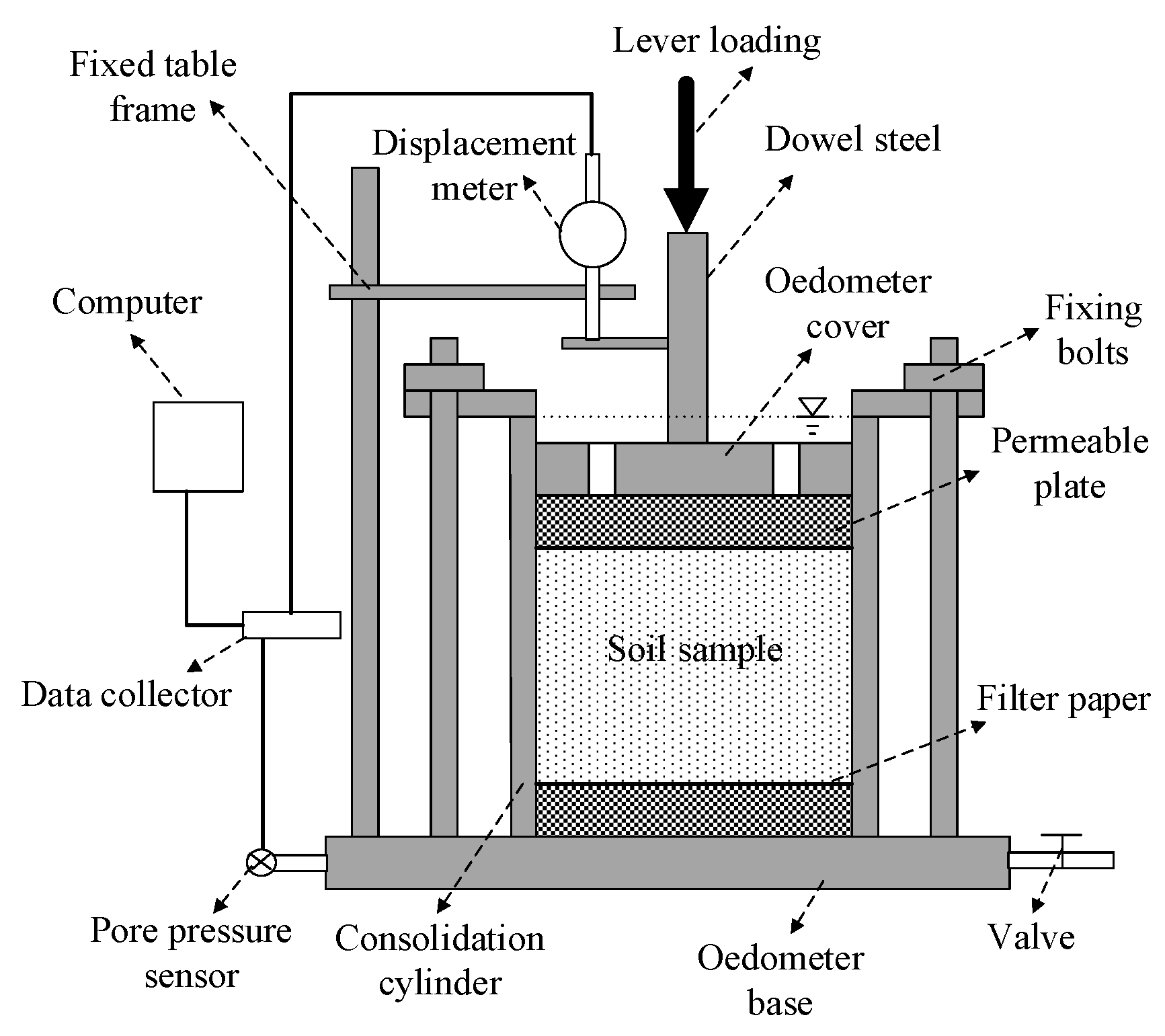
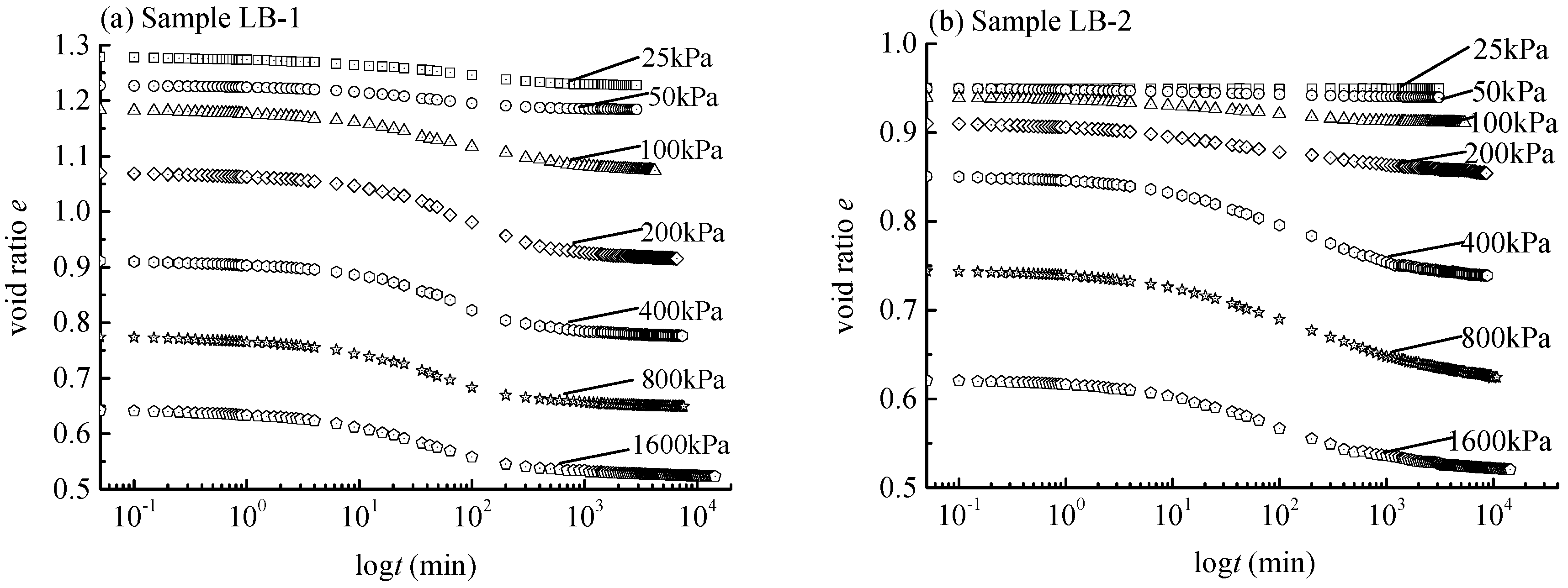
3.1. One-Dimensional Rheological Consolidation Test

In order to improve test accuracy, the TWJ-1 data collector device was introduced based on Sun’s [11] permeability-consolidation cross-test device. Displacement and pore water pressure at the bottom of the sample were measured by connecting the device to a computer. Figure 5 shows the schematic diagram of the improved consolidation device.

First, two consolidated samples were prepared as described in Section 2.2 with sample height and diameter of 2 and 6.18 cm, respectively. The basic physical parameters of the sample are summarized in Table 2. In order to simulate the rheological consolidation process of a natural saturated clay layer, the one-dimensional rheological consolidation test with upward drainage was used in this work. The loading and unloading scheme shown in Table 3 were applied based on Yin et al. [32] and Feng et al. [33]. Detailed test procedures were as follows: (1) the prepared saturated clay samples LB-1 and LB-2 were loaded into the consolidation cylinder, respectively, as shown in Figure 5. Filter paper and permeable plate are placed on the top and bottom of the samples. (2) Displacement meter and pore pressure sensor were adjusted using the data collection sofware. Then, loading was started when the displacement sensor gave values lower than 0.1 mm in a day or the pore pressure dissipated more than 95%, the next stage of loading or unloading was carried out according to

Table 4. Loading procedures in oedometer tests.

Order	Loading (kPa)
First loading	0-25-50-100-200
First Unloading	200-100-50
Second Loading	50-100-200-400
Second Unloading	400-200-100-50
Third Loading	50-100-200-400-800
Third Unloading	800-400-200-100-50
Fourth Loading	50-100-200-400-800-1600

. (3) According to the displacement sensor reading, the vertical settlement deformation S of the soil sample was calculated, and then the corresponding void ratio e was obtained according to Equation (3).

$$\log k=\log k_0-\left(e_0-e\right)/C_{\mathrm{k}}$$

(3)

where e₀ is the initial void ratio corresponding to the initial thickness H₀ of the soil sample.

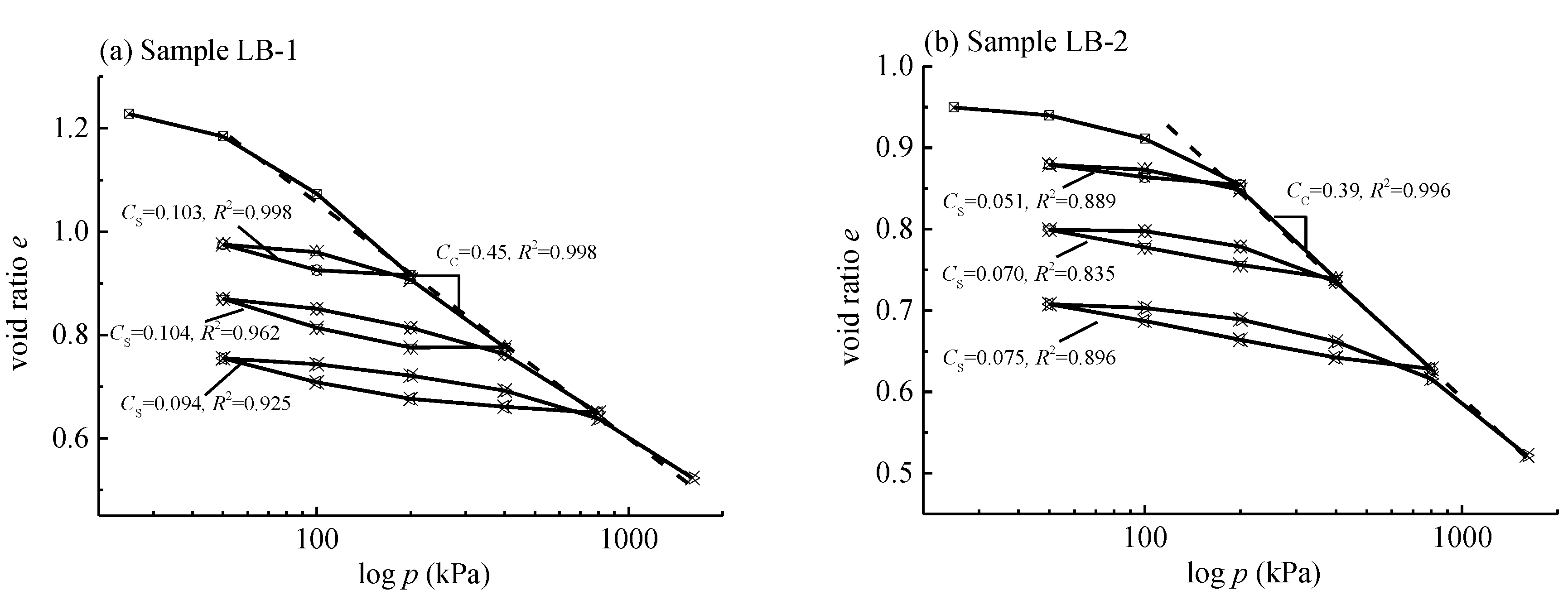
3.2. One-Dimensional Rheological Consolidation Test Data Processing

Figure 6 shows the relationship between void ratio and time-dependent loading under first-stage loading conditions. As can be seen in the figure, the obtained results were consistent with those obtained by Yin et al. [32] and Feng et al. [33] for Hong Kong clay samples; the e-logt curve had an inverse “S” shape and its tail section was elongated with the increase of vertical load. At the same time, the e-logt curve depended to some extent on the initial void ratio of the sample. As can be seen from Figure 6, by the decrease of initial void ratio, the tail section of e-logt curve became steeper and longer times were required for deformation stabilization. In addition, the slope of the tail section of the e-logt curve reflected the secondary consolidation coefficient.

Table 5. Fitting results of secondary consolidation coefficient C_α under primary loading conditions.

Soil Sample Number	Loading (kPa)
	25	50	100	200	400	800	1600
LB-1	0.0040	0.0050	0.0120	0.0110	0.0091	0.0085	0.0080
LB-2	0.0009	0.0015	0.0030	0.0092	0.0135	0.0208	0.0134

summarizes the secondary consolidation coefficient values obtained by fitting the tail section of the e-logt curve under different loads. These results are similar to those obtained by Nash et al. [28] and Chen et al. [29], where the secondary consolidation coefficient was first increased and then decreased with the increase of external load. Smaller initial void ratios of the sample gave greater consolidation coefficients. This could be attributed to the stability of clay structure at the particle’s contact surface [40].

Figure 7 shows the e-log p curves of samples LB-1 and LB-2. The curve was fitted according to the Standard for Soil Test Method (GB/T50123-1999) to obtain the values of C_c and C_s, and it was found that the average value of C_c for the two samples was 0.42. The values of C_c/C_s for samples LB-1 and LB-2 were 4.32–4.79 and 5.20–7.65, respectively. The corresponding C_c/C_s value of saturated clay was between 4.32 and 7.65, which was also obtained by Li [41] based on the GDS consolidation instrument who found C_c/C_s value of 3.65 to 7.88 for clay samples collected from the Xiaoshan in Zhejiang province. Based on the above analysis, the effectiveness of the improved oedometer proposed in this paper was verified.

4. Derivation of Governing Equations

4.1. UH Model Considering Time Effect

The above tests show that saturated soft clays have obvious rheological properties. In order to use this property in predicting consolidation behavior, a unified hardening (UH) model considering time effect was introduced [34,35] to describe the stress–strain relationship of soil. These relationships are expressed as:

$$\mathrm{d}{\epsilon }_{\mathrm{v}}=\{\begin{array}{ll}\mathrm{d}{\epsilon }_{\mathrm{v}}^{\mathrm{e}}+\mathrm{d}{\epsilon }_{\mathrm{v}}^{\mathrm{sp}}+\mathrm{d}{\epsilon }_{\mathrm{v}}^{\mathrm{tp}},\hfill & \mathrm{d}{\sigma }^{\prime }\ge 0\hfill \\ \mathrm{d}{\epsilon }_{\mathrm{v}}^{\mathrm{e}}+\mathrm{d}{\epsilon }_{\mathrm{v}}^{\mathrm{tp}},\hfill & \mathrm{d}{\sigma }^{\prime }<0\hfill \end{array}$$

(4)

where $\mathrm{d}{\epsilon }_{\mathrm{v}}$ is the vertical strain increment and $\mathrm{d}{\epsilon }_{\mathrm{v}}^{\mathrm{e}}$, $\mathrm{d}{\epsilon }_{\mathrm{v}}^{\mathrm{sp}}$ and $\mathrm{d}{\epsilon }_{\mathrm{v}}^{\mathrm{tp}}$ are elastic, plastic and time-dependent viscous strain increments caused by stress, respectively, and can be expressed as:

$$\mathrm{d}{\epsilon }_{\mathrm{v}}^{\mathrm{e}}=C_{\mathrm{s}}\mathrm{d}{\sigma }^{\prime }/\left[\ln 10\left(1+e_0\right){\sigma }^{\prime }\right]$$

(5)

$$\mathrm{d}{\epsilon }_{\mathrm{v}}^{\mathrm{sp}}=\frac{C_{\mathrm{c}}-C_{\mathrm{s}}}{\ln 10\left(1+e_0\right)}\frac{M^4}{M_{\mathrm{f}}^4}\frac{\mathrm{d}{\sigma }^{\prime }}{{\sigma }^{\prime }}$$

(6)

$$\mathrm{d}{\epsilon }_{\mathrm{v}}^{\mathrm{tp}}=C_{\mathsf{\alpha }}\mathrm{d}t/\left[\ln 10\left(1+e_0\right)\left(t_{\mathsf{\alpha }}+t_0\right)\right]$$

(7)

where $C_{\mathrm{c}}$ is the compressed index, $C_{\mathrm{s}}$ is the swelling index, $C_{\mathsf{\alpha }}$ is the secondary consolidation coefficient, $t_{\mathsf{\alpha }}$ is the aging time, $t_0$ is the unit time which can be 1 s, 1 min, 1 h, etc. According to actual situations, $M$ is the stress ratio at critical state and $M_{\mathrm{f}}$ is the potential failure stress ratio, which can be expressed as:

$$M=6\sin \phi /\left(3-\sin \phi \right)$$

(8)

$$M_{\mathrm{f}}=6\left[\sqrt{\chi /R\left(1+\chi /R\right)}-\chi /R\right]$$

(9)

$$\left(t_{\mathrm{a}}+t_0\right)/t_0=R^{-\mathsf{\alpha }}$$

(10)

$$R=\frac{{\sigma }^{\prime }}{{p^{\prime }}_{\mathrm{c}}}\exp \left(-\frac{\ln 10·\left(1+e_0\right){\epsilon }_{\mathrm{v}}^{\mathrm{p}}}{C_{\mathrm{c}}-C_{\mathrm{s}}}\right)$$

(11)

where $\phi$ is the internal friction angle of soil, $\chi =M^2/12\left(3-M\right)$, $\alpha =\left(C_{\mathrm{c}}-C_{\mathrm{s}}\right)/C_{\mathsf{\alpha }}$, and R is a parameter reflecting the degree of over-consolidation. When time effect is not considered, the initial value R₀ is reciprocal of the over-consolidation ratio (OCR). ${\epsilon }_{\mathrm{v}}^{\mathrm{p}}$ is the plastic strain produced by stress and time, ${p^{\prime }}_{\mathrm{c}}$ is the vertical stress at the intersection of rebound and instantaneous compression lines, similar to pre-consolidation pressure.

4.2. One-Dimensional Rheological Consolidation Equation of UH Model

First, the principle of effective stress is obtained as:

$${\sigma }^{\prime }={{\sigma }^{\prime }}_0+p_0-u$$

(12)

where ${{\sigma }^{\prime }}_0$ is the initial effective stress, $p_0$ is the external loads, and $u$ is the excess pore water pressure. For both sides of Equation (12), partial derivatives could be obtained at the same time as:

$$\frac{\partial {\sigma }^{\prime }}{\partial z}=-\frac{\partial u}{\partial z}$$

(13)

Based on continuous conditions of permeability we had:

$$\frac{\partial q}{\partial z}=-\frac{\partial {\epsilon }_{\mathrm{v}}}{\partial t}$$

(14)

where q is the change of water quantity within the unit cell during an infinitesimal time period of dt can be expressed as $q=vA$, A is the area of water flowing through the unit cell.

Substituting Equations (1), (2), (4), and (13) into Equation (14) gives:

$$\frac{\partial }{\partial z}\left(\psi \frac{\partial {\sigma }^{\prime }}{\partial z}\right)=\beta \frac{\partial {\sigma }^{\prime }}{\partial t}+\eta$$

(15)

where $\eta ={\gamma }_{\mathrm{w}}{C}_{\mathsf{\alpha }}/\left[\ln 10k_0\left(1+e_0\right)\left(t_{\mathsf{\alpha }}+t_0\right)\right]$, $\psi =\{\begin{array}{cc}\frac{\exp \left[-\ln 10{\epsilon }_{\mathrm{v}}\left(1+e_0\right)/C_{\mathrm{k}}\right]}{m{\left({\gamma }_w{i}_1\right)}^{m-1}}·{\left|\frac{\partial {\sigma }^{\prime }}{\partial z}\right|}^{m-1},\hfill & \hspace{1em}\left|i\right|\le i_1\hfill \\ \exp \left[-\ln 10{\epsilon }_{\mathrm{v}}\left(1+e_0\right)/C_{\mathrm{k}}\right],\hfill & \left|i\right|>i_1\hfill \end{array}$, $\beta =\{\begin{array}{cc}\frac{\left[C_{\mathrm{S}}+\left(C_{\mathrm{C}}-C_{\mathrm{S}}\right)M^4/M_{\mathrm{f}}^4\right]{\gamma }_{\mathrm{w}}}{\left(1+e_0\right)k_0{\sigma }^{\prime }\ln 10},\hfill & \mathrm{d}{\sigma }^{\prime }\ge 0\hfill \\ \frac{C_{\mathrm{S}}{\gamma }_{\mathrm{w}}}{\left(1+e_0\right)k_0{\sigma }^{\prime }\ln 10},\hfill & \mathrm{d}{\sigma }^{\prime }<0\hfill \end{array}$

However, the initial and boundary conditions of the device shown in Figure 4 are expressed as:

$${\sigma }^{\prime }\left(z,0\right)={{\sigma }^{\prime }}_0,0\le z\le H\left(\mathrm{initial}\mathrm{condition}\right)$$

(16)

$${\sigma }^{\prime }\left(0,t\right)=p_0+{{\sigma }^{\prime }}_0,t>0\left(\mathrm{permeable}\mathrm{boundary}\right)$$

(17)

$${\frac{\partial {\sigma }^{\prime }}{\partial z}|}_{z=H}=0,t>0(\mathrm{imperious}\mathrm{boundary})$$

(18)

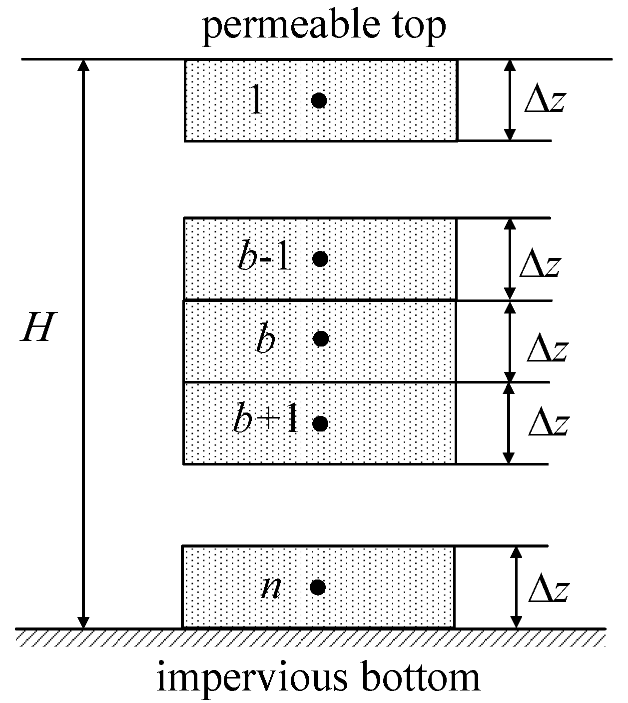
4.3. Discretization of the Governing Equation

Due to the complexity of Equation (15), it was very difficult to obtain its analytical solution. Therefore, the numerical solutions can be obtained using the finite difference method (FDM), finite volume method (FVM), or finite element method (FEM). It was found that among these methods, the FVM was a numerical solution based on FDM, and absorbs the advantages of the FEM. Some researchers have studied this method [15,42] and their results showed that FVM as more advantages than FDM and FVM in terms of convergence and accuracy. Therefore, FVM was used in this paper to solve the problem.

To obtain numerical solutions for Equation (15) using FVM, as shown in Figure 8, the spatial domain 0 ≤ z ≤ H was firstly divided into n thin layers with equal length Δz. Meanwhile, the time axis is divided by a series of time increments Δt. Where bth is the number of spatial nodes, jth is time discretized point. Then, within any time interval Δt (t_j to t_j+1), Equation (15) was integrated in the control volume of bth:

$${\displaystyle {\int }_{t_j}^{t_{j+1}}{\displaystyle \underset{\Delta z}{\int }\frac{\partial }{\partial z}\left(\psi \frac{\partial {\sigma }^{\prime }}{\partial z}\right)}}\mathrm{d}z\mathrm{d}t={\displaystyle {\int }_{t_j}^{t_{j+1}}{\displaystyle \underset{\Delta z}{\int }\left(\beta \frac{\partial {\sigma }^{\prime }}{\partial t}+\eta \right)}}\mathrm{d}z\mathrm{d}t$$

(19)

Equation (19) can be rewritten as:

$${\displaystyle {\int }_{t_j}^{t_{j+1}}\left({\psi \frac{\partial {\sigma }^{\prime }}{\partial z}|}_B-{\psi \frac{\partial {\sigma }^{\prime }}{\partial z}|}_D\right)}\mathrm{d}z\mathrm{d}t={\displaystyle {\int }_{t_j}^{t_{j+1}}{\displaystyle \underset{\Delta z}{\int }\left(\beta \frac{\partial {\sigma }^{\prime }}{\partial t}+\eta \right)}}\mathrm{d}z\mathrm{d}t$$

(20)

where the subscripts B and D represent the lower and upper boundary points of the control volume, respectively.

For Equation (20), the first-order forward difference is used to approximate the right side of the equal sign $\partial {\sigma }^{\prime }/\partial t$ and the central difference is used to approximate the left side of the equal sign $\partial {\sigma }^{\prime }/\partial z$. To describe the relationship between ${{\sigma }^{\prime }}_{b-1}$, ${{\sigma }^{\prime }}_b$, ${{\sigma }^{\prime }}_{b+1}$, and time, the effective stresses at $t_j$ and $t_{j+1}$ are usually weighted as a combination and then taken as the average value of the time from $t_j$ to $t_{j+1}$. Then, the time integral term on the left side of Equation (20) is calculated. Where the weight of $t_j$ is 0 and that of $t_{j+1}$ is 1. That is to say, Equation (20) can be written as:

$$\left[{\psi }_{b+1/2}^{j+1}\left(\frac{{{\sigma }^{\prime }}_{b+1}^{j+1}-{{\sigma }^{\prime }}_b^{j+1}}{\Delta z}\right)-{\psi }_{b-1/2}^{j+1}\left(\frac{{{\sigma }^{\prime }}_b^{j+1}-{{\sigma }^{\prime }}_{b-1}^{j+1}}{\Delta z}\right)\right]\Delta t={\beta }_b^{j+1}({{\sigma }^{\prime }}_b^{j+1}-{{\sigma }^{\prime }}_b^j)\Delta z+{\eta }_b^{j+1}\Delta z\Delta t$$

(21)

Equation (21) is reorganized as:

$${{\sigma }^{\prime }}_b^{j+1}={{\sigma }^{\prime }}_b^j+\left[{\psi }_{b+1/2}^{j+1}({{\sigma }^{\prime }}_{b+1}^{j+1}-{{\sigma }^{\prime }}_b^{j+1})-{\psi }_{b-1/2}^{j+1}({{\sigma }^{\prime }}_b^{j+1}-{{\sigma }^{\prime }}_{b-1}^{j+1})\right]\Delta t/({\beta }_b^{j+1}\Delta z^2)-{\eta }_b^{j+1}\Delta t/{\beta }_b^{j+1}$$

(22)

where b is the number of spatial nodes, j is time discretized point, $x_b^j$ represents the value of $x$ variable at $z=\left(b-1/2\right)\Delta z$ and $t=j\Delta t$, $x_{b\pm 1/2}^j$ represents the value of $x$ variable at $z=\left(b-1/2\pm 1/2\right)$ and $t=j\Delta t$, the same below.

With the above-mentioned method (FVM), Equations (16)–(18) can be discretized as:

$${{\sigma }^{\prime }}_b^0={{\sigma }^{\prime }}_0,b=1,2,3,\dots ,n$$

(23)

$${{\sigma }^{\prime }}_1^{j+1}={{\sigma }^{\prime }}_1^j+\left[{\psi }_{3/2}^{j+1}({{\sigma }^{\prime }}_2^{j+1}-{{\sigma }^{\prime }}_1^{j+1})-2{\psi }_{1/2}^{j+1}({{\sigma }^{\prime }}_1^{j+1}-p_0-{{\sigma }^{\prime }}_0)\right]\Delta t/({\beta }_1^{j+1}·\Delta z^2)-\Delta t·{\eta }_1^{j+1}/{\beta }_1^{j+1}$$

(24)

$${{\sigma }^{\prime }}_n^{j+1}={{\sigma }^{\prime }}_n^j-{\psi }_{n-1/2}^{j+1}({{\sigma }^{\prime }}_n^{j+1}-{{\sigma }^{\prime }}_{n-1}^{j+1})\Delta t/({\beta }_n^{j+1}\Delta z^2)-{\eta }_n^{j+1}\Delta t/{\beta }_n^{j+1}$$

(25)

Thus, Equations (22)–(25) composed a closed system of equations, and the exact solutions for unknown variables ${{\sigma }^{\prime }}_b^{j+1}$ can be obtained using the method of iteration.

In order to analyze the settlement deformation law of foundation, settlement at time t is expressed as:

$$S_t={\displaystyle {\int }_0^H{\epsilon }_{\mathrm{v}}\left(z,t\right)}\mathrm{d}z=\Delta z·{\displaystyle \sum _{b=1}^n{\epsilon }_{\mathrm{v}}{}_b^{j+1}}$$

(26)

where H is the thickness of foundation soil or the soil sample’s initial height, and ${\epsilon }_{\mathrm{v}}\left(z,t\right)$ is the vertical strain of foundation or soil sample at any depth z and time t.

5. Verification of the Suitability of UH Model

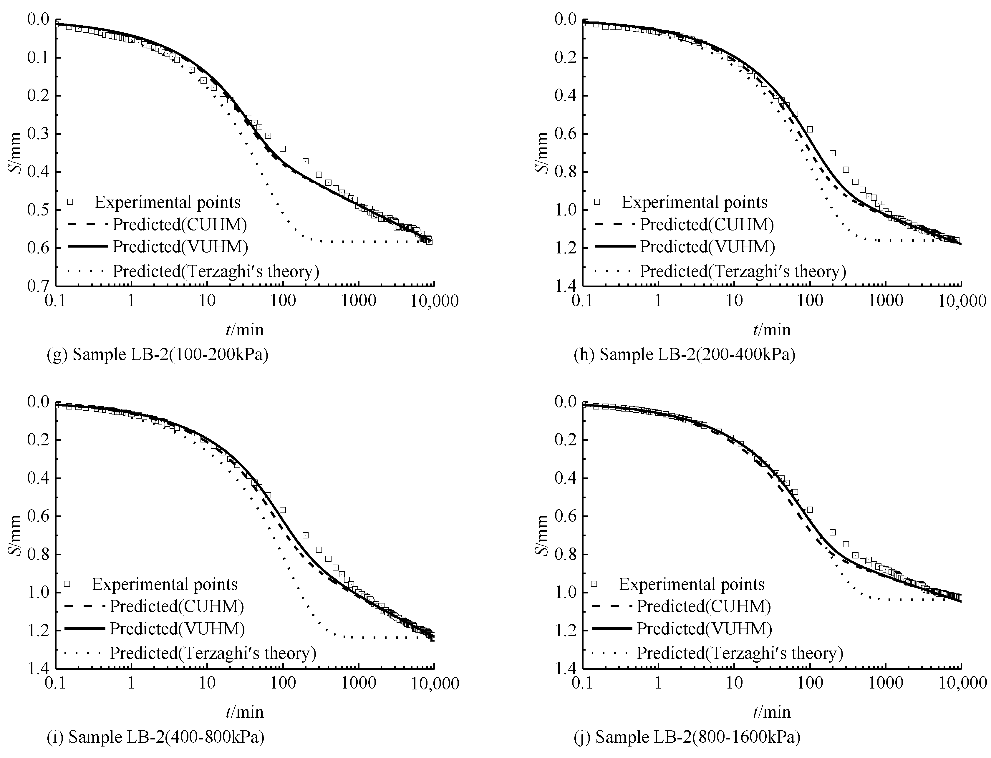
5.1. Verification of the Experimental Results in this Paper

First, a code is written in the Fortran software according to the above algorithm. The test results obtained for samples LB-1 and LB-2 are then used as input. Since the test sample’s thickness is small, the effect of Hansbo’s flow can be neglected [14] and analysis can be performed based on Darcy’s flow; i.e., m = 1.0 or i₁ = 0. The compression index C_c, swelling index C_s, and secondary consolidation coefficient C_α are taken according to the above test results. Sorensen et al. [43] summarized some clay experimental data on clay and provided the relationship between the internal friction angle φ and plasticity index I_P, as shown in Equation (27). Therefore, φ = 25° can be estimated based on Equation (27) and Table 1 (I_P = 17.1), and then M = 0.984 can be obtained by substituting φ into Equation (8). Moreover, the initial permeability coefficient k₀, permeation index C_k, and initial over-consolidation parameter R₀ were selected by trial calculation, as shown in

Table 6. UH model parameters of sample LB-1.

Loading Interval/(kPa)	H/mm	e0	CC	Ck	CS	Cα	R0	k0/(m/min)
50–100	18.99	1.184	0.42	0.66	0.100	0.0120	0.65	1.2 × 10−8
100–200	18.01	1.070				0.0110	0.92	0.70 × 10−8
200–400	16.63	0.913				0.0091	0.83	0.40 × 10−8
400–800	15.44	0.776				0.0085	0.79	0.25 × 10−8
800–1600	14.29	0.644				0.0080	0.76	0.12 × 10−8

and

Table 7. UH model parameters of sample LB-2.

Loading Interval/(kPa)	H/mm	e0	CC	Ck	CS	Cα	R0	k0/(m/min)
50–100	1.988	0.940	0.42	0.66	0.065	0.0030	0.58	1.0 × 10−8
100–200	1.959	0.911				0.0092	0.53	0.85 × 10−8
200–400	1.899	0.852				0.0135	0.65	0.39 × 10−8
400–800	1.789	0.745				0.0190	0.60	0.19 × 10−8
800–1600	1.512	0.622				0.0135	0.66	0.06 × 10−8

. Numerical simulation results are shown in Figure 9, which shows that the predicted results from the UH model, considering the time effect, are in good agreement with the experimental results. However, the predicted results of Terzaghi’s theory are quite different from the experimental results in the later stage of loading. The above results fully prove the necessity of considering the soil’s rheological characteristics in predicting foundation settlement in saturated clay areas, and also proved the UH model’s applicability and the necessity of considering variable permeability coefficient.

$$\phi =\{\begin{array}{cc}43-10·\log \left(I_{\mathrm{P}}\right),\hfill & \left(\mathrm{mean}\right)\hfill \\ 39-11·\log \left(I_{\mathrm{P}}\right),\hfill & \left(\mathrm{lower}\mathrm{bound}\right)\hfill \end{array}$$

(27)

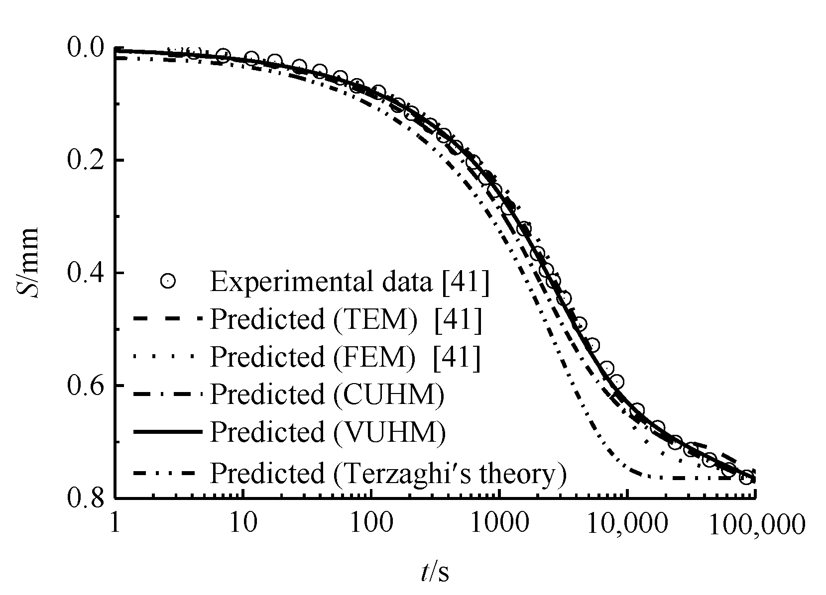
5.2. Verification of Experimental Results obtained by Li's

Li [41] conducted one-dimensional consolidation tests on clay samples collected from Xiaoshan, Zhejiang province using an advanced GDS consolidation instrument, introduced the three-element model (TEM) and four-element model (FEM) (can been seen Figure 10) into one-dimensional consolidation analysis, and verified the obtained results by comparing them to the experimental results. Hu et al. [35] used the test data of samples 3 and 4 under loading stages of 800–1,600 kPa [41] to verify the UH model’s applicability, but did not consider the permeability coefficient’s influence. The same UH model parameters as those listed in [35] were used in this work as H = 14.8 mm, e₀ = 0.82, C_C = 0.356, C_k = 0.528, C_S = 0.073, C_α = 0.011, k₀ = 2.0 × 10⁻¹¹ m/s, M = 0.984, and R₀ = 0.575. The comparison of theoretical and experimental values based on the proposed model is shown with Figure 11. It can be seen that the results obtained from the UH model considering the variable permeability coefficient are closer to experimental values compared to those from the component model, which fully confirms superiority of the UH model and the necessity of considering the permeability coefficient in similar studies.

6. Conclusions

In this paper, we used an improved constant-head permeameter to measure the permeability coefficient of fine-grained soil rapidly and accurately at insignificant amounts of water flow rate. The improved oedometer is used to verify the significant rheological properties of saturated clay. Then the one-dimensional rheological consolidation equation based on Hansbo’s flow and the UH model considering the time effect is derived, and the numerical solution of FVM is given. Finally, the numerical simulation results are compared to the experimental results, and the following conclusions are drawn:

(1)

Compared to the traditional falling-head permeability experiment, the improved constant-head experimental device for insignificant amounts of water flow saturated clays requires shorter time and has less experimental error.

(2)

The water flow of saturated clay pores deviated from Darcy flow and Hansbo’s flow equations had good applicability to clay samples used in this experiment.

(3)

Saturated clay had significant rheological properties. The predicted results of Terzaghi’s theory were quite different from the experimental results, and the UH constitutive model agreed well with experimental results and had good applicability in predicting the rheological deformation of saturated clay samples.

The graduated U-tube with a 4 mm inner diameter and a video device were used to improve the conventional constant-head permeability test device to provide accurate and fast measurement of permeability coefficient of saturated clays under the condition of insignificant amounts of water flow, saves considerable experimental time, and avoids the experimental errors caused by environmental and human factors. The unified hardening (UH) constitutive model considering the time effect was introduced to describe the rheological properties of saturated clay soils, and Hansbo’s equation was employed to describe the non-Darcian flow in the process of consolidation. Accordingly, Terzaghi’s one-dimensional consolidation theory of saturated clay was modified and numerical analysis was conducted using FVM. Comparing the numerical simulation and experimental results, the applicability of the UH model considering time effects and the necessity of considering variable permeability coefficient were verified.

7. Patents

• Zhongyu Liu; Yangyang Xia; Jiachao Zhang; Xinmu Zhu; Jiandong Wei. A device for preparing saturated remolded clay ring knife sample. China Patent, CN201,721,820,336.8, 2018-08-07.
• Jiandong Wei; Yangyang Xia; Zhongyu Liu; Jiachao Zhang; Xinmu Zhu. A triple saturated clay constant-head permeability test device. China Patent, CN201,821,335,366.4, 2019-04-12.

References

1. Terzaghi, K. Theoretical Soil Mechanics; Wiley and Sons: New York, NY, USA, 1943. [Google Scholar]
2. King, F.H. Principles and Conditions of the Movement of Ground Water; United States Geological Survey: Reston, VA, USA, 1898. [Google Scholar]
3. Hansbo, S. Consolidation of clay with special reference to influence of vertical sand drain. Swed. Geotech. Inst. 1960, 18, 45–50. [Google Scholar]
4. Swartzendruber, D. Modification of darcy’s law for the flow of water in soils. Soil Sci. 1962, 93, 22–29. [Google Scholar] [CrossRef]
5. Slepicka, F. Contribution to the Solution of the Filtration Law; International Union of Geodesy and Geophysics, Commission of Subterranean Waters: Helsinkl, Finland, 1960; pp. 245–258. [Google Scholar]
6. Miller, R.J.; Low, P.E. Threshold gradient for water flow in clay systems. Soil Sci. Soc. Am. J. 1963, 27, 605–609. [Google Scholar] [CrossRef]
7. Qi, T.; Xie, K.H.; Hu, A.F.; Zhang, Z.Q. Laboratorial study on non-Darcy permeability in Xiaoshan clay. J. Zhejiang Univ. Eng. Sci. 2007, 41, 1023–1028. [Google Scholar]
8. Dubin, B.; Moulin, G. Influence of a critical gradient on the consolidation of clays. In Consolidation of Soils: Testing and Evaluation (STP 892); ASTM: West Conshochen, PA, USA, 1986; pp. 354–377. [Google Scholar]
9. Wang, X.Y.; Liu, C.L. New understanding of the regularity of water permeability in cohesive soil. Acta Geosci. Sin. 2003, 24, 91–95. [Google Scholar]
10. Deng, Y.E.; Xie, H.P.; Huang, R.Q.; Liu, C.Q. Law of nonlinear flow in saturated clays and radial consolidation. Appl. Math. Mech. 2007, 28, 1427–1436. [Google Scholar] [CrossRef]
11. Sun, L.Y.; Yue, J.C.; Zhang, J. Experimental study on non-Darcian permeability characteristics of saturated clays. J. Zhengzhou Univ. Eng. Sci. 2010, 31, 31–34. [Google Scholar]
12. Hansbo, S. Deviation from Darcy’s law observed in one dimensional consolidation. Geotechnique 2003, 53, 601–605. [Google Scholar] [CrossRef]
13. E, J.; Chen, G.; Sun, A.R. One-dimensional consolidation of saturated cohesive soil considering non-Darcy flows. Chin. J. Geotech. Eng. 2009, 31, 1115–1119. [Google Scholar]
14. Li, C.X.; Xie, K.H. One-dimensional nonlinear consolidation of soft clay with the non-Darcian flow. J. Zhejiang Univ. Sci. 2013, 14, 435–446. [Google Scholar] [CrossRef] [Green Version]
15. Liu, Z.Y.; Sun, L.Y.; Yue, J.C.; Ma, C.W. One-dimensional consolidation theory of saturated clay based on non-Darcy flow. Chin. J. Rock Mech. Eng. 2009, 28, 973–979. [Google Scholar]
16. Liu, Z.Y.; Zhang, J.C.; Zheng, Z.L.; Guan, C. Finite element analysis of two-dimensional Biot’s consolidation with Hansbo’s flow. Rock Soil Mech. 2018, 39, 4617–4626. [Google Scholar]
17. Liu, Z.Y.; Jiao, Y. Consolidation of ground with ideal sand drains based on Hansbo’s flow. Chin. J. Geotech. Eng. 2015, 37, 792–801. [Google Scholar]
18. Davis, E.H.; Raymond, G.P. A non-linear theory of consolidation. Géotechnique 1965, 15, 161–173. [Google Scholar] [CrossRef]
19. Zhuang, Y.C.; Xie, K.H.; Li, X.B. Nonlinear analysis of consolidation with variable compressibility and permeability. J. Zhejiang Univ. Eng. Sci. 2005, 6, 181–187. [Google Scholar] [CrossRef]
20. Conte, E. Consolidation of anisotropic soil deposits. Soils Found. 1998, 38, 227–237. [Google Scholar] [CrossRef]
21. Bartholomeeusen, G.; Sills, G.C.; Znidarčiċ, D.; Van Kesteren, W.; Merckelbach, L.M.; Pyke, R.; Carrier, W.D.; Lin, H.; Penumadu, D.; Winterwerp, H.; et al. Sidere: Numerical prediction of large-strain consolidation. Géotechnique 2002, 52, 639–648. [Google Scholar] [CrossRef]
22. Conte, E.; Troncone, A. Nonlinear consolidation of thin layers subjected to time-dependent loading. Can. Geotech. J. 2007, 44, 717–725. [Google Scholar] [CrossRef]
23. Buisman, A.S. Results of long duration settlement tests. In Proceedings of the 1th International Conference on Soil Mechanics and Foundation Engineering, Cambridge, MA, USA, 22–26 June 1936; pp. 103–105. [Google Scholar]
24. Taylor, D.W.; Merchant, W. A theory of clay consolidation accounting for secondary compression. J. Math. Phys. 1940, 19, 167–185. [Google Scholar] [CrossRef]
25. Chen, Z.J. One dimensional problems of consolidation and secondary time effects. China Civ. Eng. J. 1958, 5, 1–3. [Google Scholar]
26. Bjerrum, L. Engineering geology of normally consolidated marine clays as related to the settlement of buildings. Geotechnique 1967, 17, 83–118. [Google Scholar] [CrossRef]
27. Bjerrum, L. Embankments on soft ground: State of threat report. In Proceedings of the Specialty Conference on Performance of Earth and Earth Supported Structures, Lafayette, Indiana, 11–14 June 1972; pp. 1–54. [Google Scholar]
28. Nash, D.F.T.; Sills, G.C.; Davison, L.R. One-dimensional consolidation testing for soft clay from Bothkennar. Geotechnique 1992, 42, 241–256. [Google Scholar] [CrossRef]
29. Chen, X.P.; Luo, Q.Z.; Zhou, Q. Time-dependent behaviour of interactive marine and terrestrial deposit clay. Geomech. Eng. 2014, 7, 279–295. [Google Scholar] [CrossRef]
30. Yin, Z.Z.; Zhang, H.B.; Zhu, J.G.; Li, G.W. Secondary consolidation of soft soils. Chin. J. Geotech. Eng. 2003, 25, 521–526. [Google Scholar]
31. Reddy, B.K.; Sahu, R.B.; Ghosh, S. Consolidation behavior of organic soil in normal Kolkata Deposit. Indian Geotech. J. 2014, 44, 341–350. [Google Scholar] [CrossRef]
32. Yin, J.H. Non-linear creep of soils in oedometer tests. Geotechnique 1999, 49, 699–707. [Google Scholar] [CrossRef]
33. Feng, W.Q.; Lalit, B.; Yin, Z.Y.; Yin, J.H. Long-term Non-linear creep and swelling behavior of Hong Kong marine deposits in oedometer condition. Comput. Geotech. 2017, 84, 1–15. [Google Scholar] [CrossRef]
34. Yao, Y.P.; Kong, L.M.; Hu, J. An elastic-viscous-plastic model for overconsolidated clays. Sci. China Tech. Sci. 2013, 56, 441–457. [Google Scholar] [CrossRef]
35. Hu, J.; Yao, Y.P. One-dimensional consolidation analysis of UH model considering time effect. J. Beijing Univ. Aeronaut. Astronaut. 2015, 41, 1492–1498. [Google Scholar]
36. GB/T50123-1999. Standard for Soil Test Method; China Planning Press: Beijing, China, 1999. [Google Scholar]
37. Liu, Z.Y.; Xia, Y.Y.; Zhang, J.C.; Zhu, X.M.; Wei, J.D. Preparation Device for Saturated Remodeling Clay Soil Ring Knife Sample. China Henan CN207703568U, 7 August 2018. [Google Scholar]
38. Taylor, D.W. Fundamentals of Soil Mechanics; John Wiley & Sons Inc.: New York, NY, USA, 1948. [Google Scholar]
39. Beery, P.L.; Wilkinson, W.B. The radial consolidation of caly soils. Geotechnique 1969, 19, 253–254. [Google Scholar] [CrossRef]
40. Wong, R.C.; Varatharajan, S. Viscous behaviour of clays in one-dimensional compression. Can. Geotech. J. 2014, 51, 795–809. [Google Scholar] [CrossRef]
41. Li, X.B. Theoretical and Experimental Studies on Rheological Consolidation of Soft Soil; Zhejiang University: Hangzhou, China, 2005. [Google Scholar]
42. Chen, F.; Drumm, E.C.; Guiochon, G. Coupled discrete element and finite volume solution of two classical soil mechanics problems. Comput. Geotech. 2011, 38, 638–647. [Google Scholar] [CrossRef]
43. Sorensen, K.K.; Okkels, N. Correlation between Drained Shear Strength and Plasticity Index of Undisturbed Overconsolidated Clays. In Proceedings of the 18th International Conference on Soil Mechanics and Geotechnical Engineering, Paris, France, 2–6 September 2013; Volume 1, pp. 423–428. [Google Scholar]
Figure 1. Falling-head permeability test results.
Water 11 01385 g001
Figure 2. Schematic diagram of the improved constant-head permeability test device.
Water 11 01385 g002
Figure 3. Comparison of experimental results and those obtained from Hansbo’s flow fitting.
Water 11 01385 g003
Figure 4. The relationship between the permeability coefficient k and void ratio e.
Water 11 01385 g004
Figure 5. Schematic diagram of the improved oedometer.
Water 11 01385 g005
Figure 6. e-logt curves of samples LB-1 and LB-2 under primary loading condition.
Water 11 01385 g006
Figure 7. e-log p (vertical load) curves for samples LB-1 and LB-2.
Water 11 01385 g007
Figure 8. Discretized schematic of the soil layer.
Water 11 01385 g008
Figure 9. Comparison of theoretical and experimental settlement values for samples LB-1and LB-2. CUHM: unified hardening model with constant permeability coefficient, VUHM: unified hardening model with variable permeability coefficient.
Water 11 01385 g009aWater 11 01385 g009b
Figure 10. Schematic diagram of rheological model (a): three-element rheological model, (b) Four-element rheological model. where E0 and E1 are the moduli of the independent spring and the spring of the Kelvin–Voigt body, respectively; η0 and η1 are the viscosity coefficient of the independent dashpot and the dashpot of the Kelvin–Voigt body, respectively.
Water 11 01385 g010
Figure 11. Comparison of prediction values and experimental results of the settlement theory under different models.
Water 11 01385 g011