Analysis of the Effect of Uncertainty in Rainfall-Runoff Models on Simulation Results Using a Simple Uncertainty-Screening Method

Abstract
1. Introduction
2. Materials
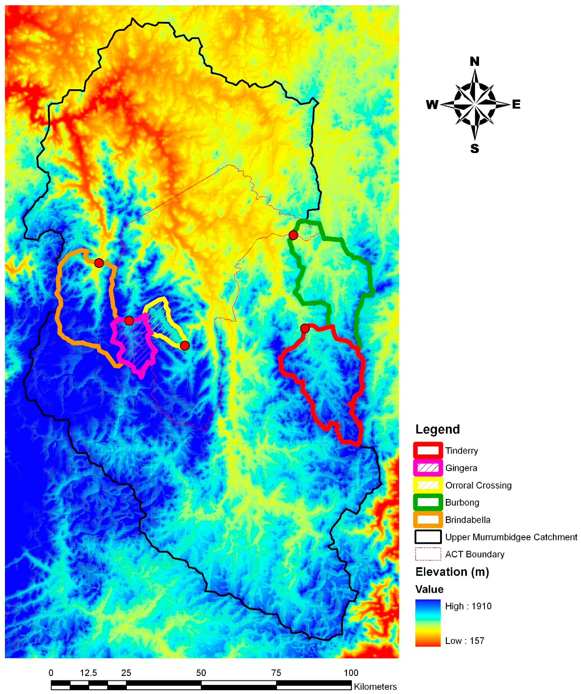
2.1. Catchments
2.2. Data
2.3. Rainfall-Runoff Models
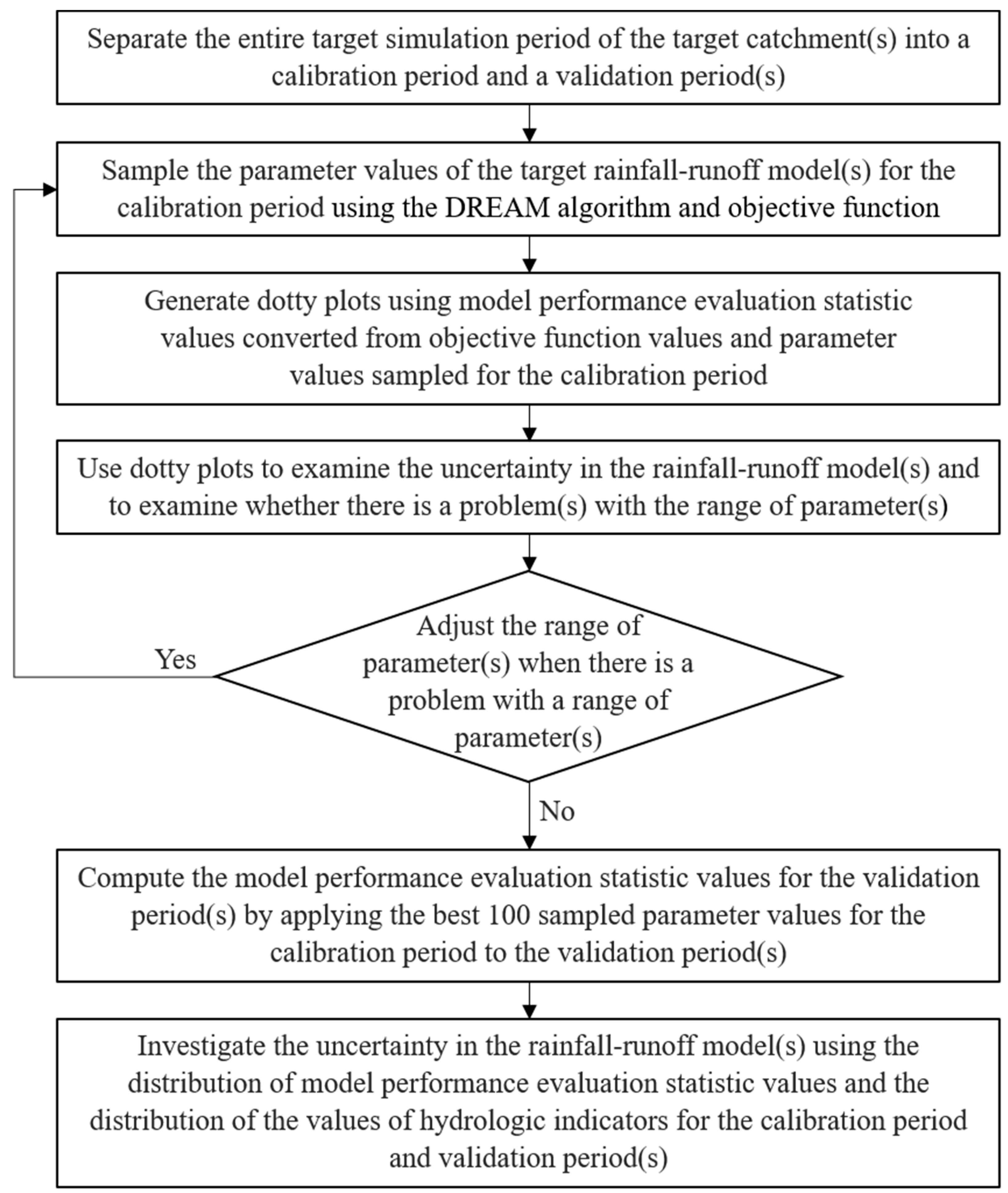
3. Method
3.1. Sampling of Parameters Using the Differential Evolution Adaptive Metropolis Algorithm
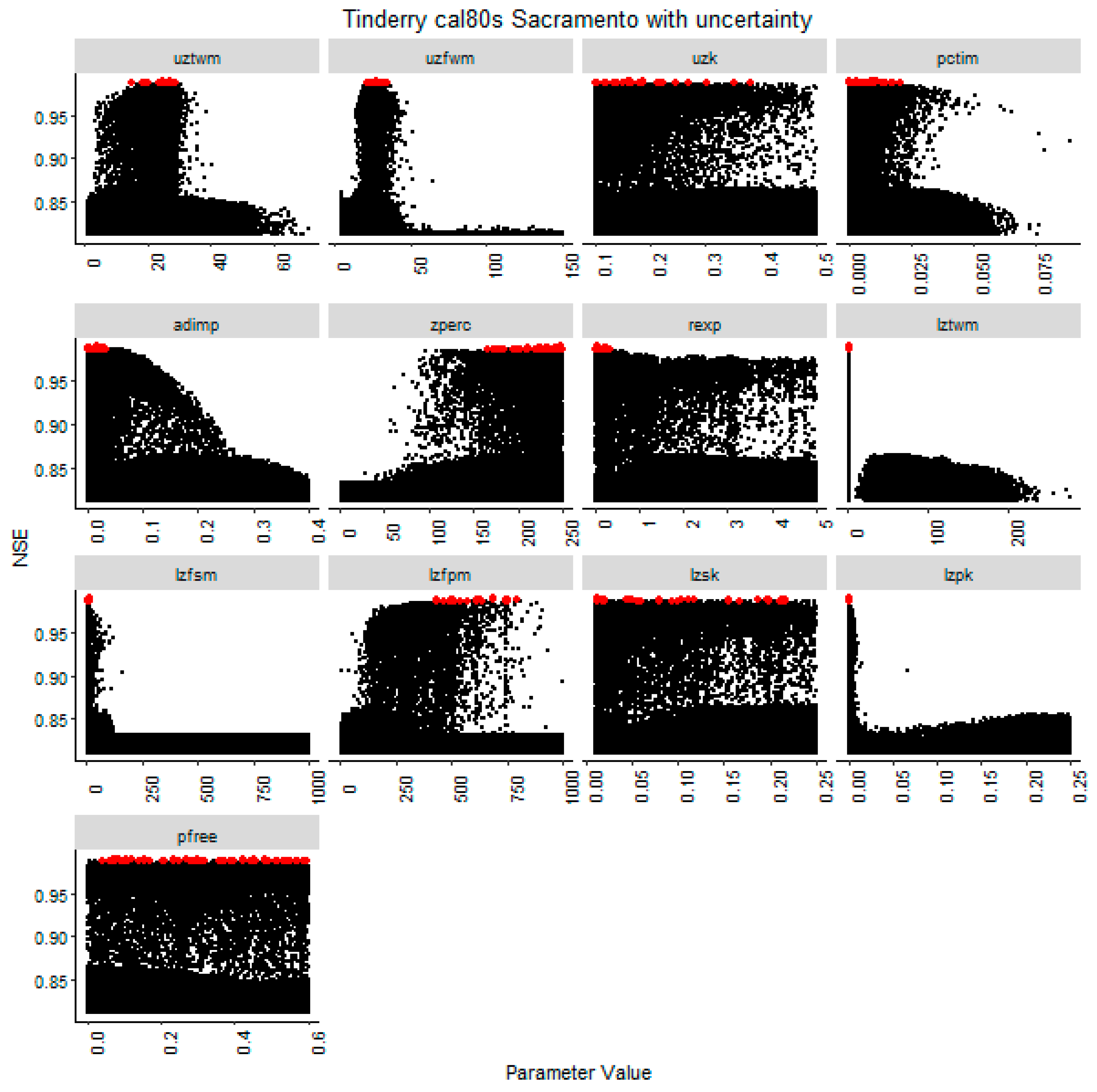
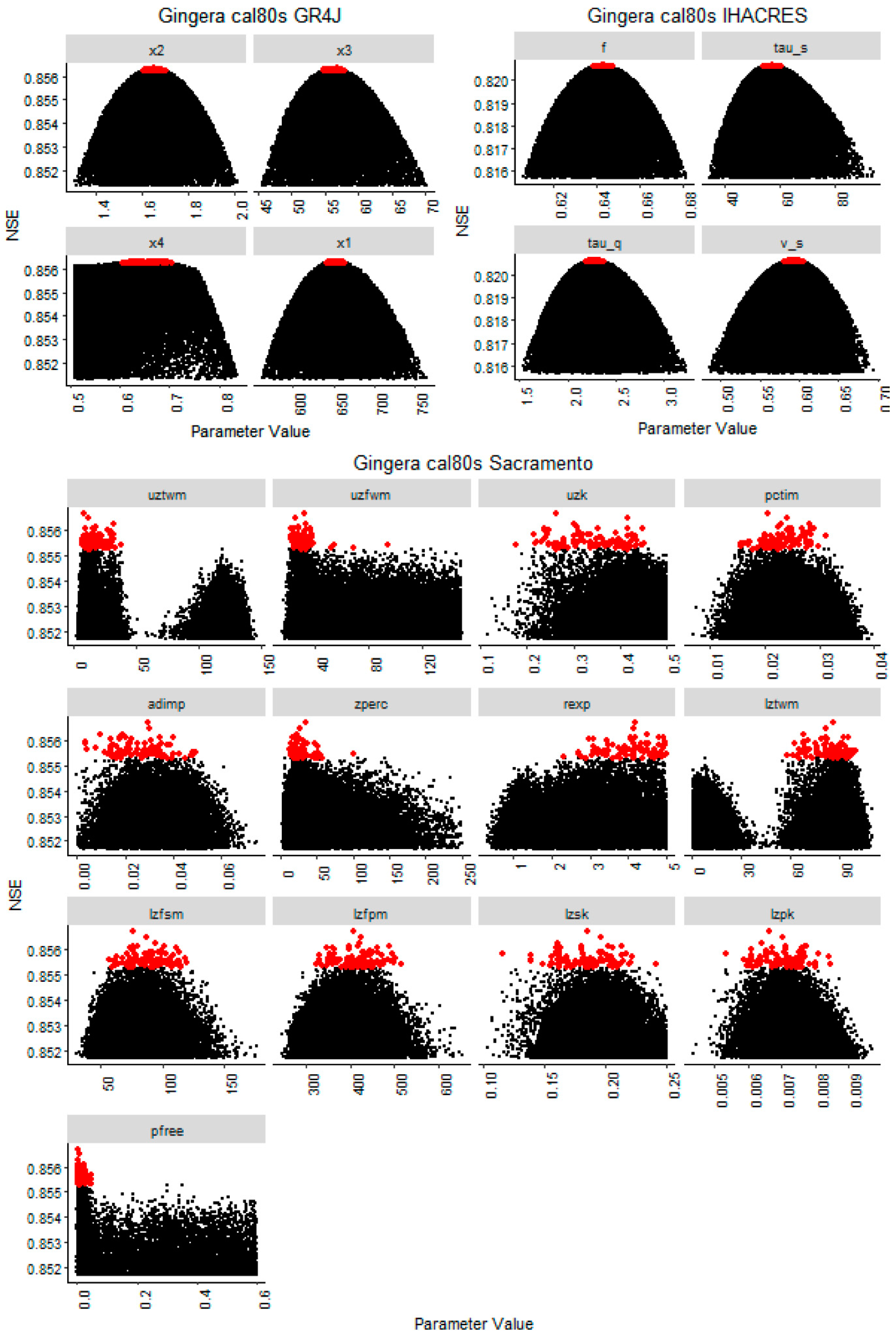
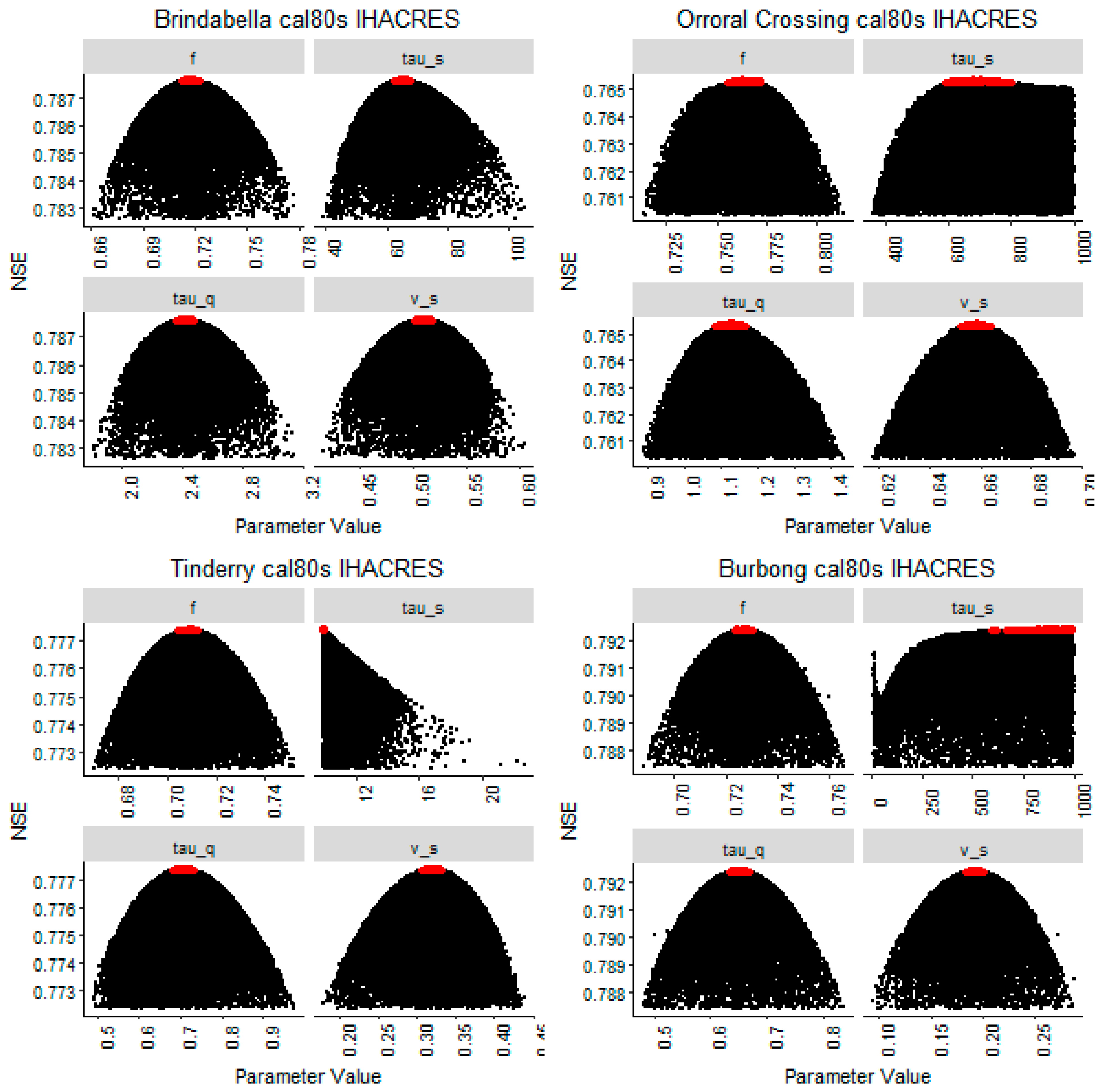
3.2. Investigation of Sampled Parameters Using Dotty Plots
3.3. Applying the 100 Best Equifinal Calibrated Parameter Values to Validation Periods to Investigate Uncertainty in Model Structures
3.4. Investigation of Hydrologic Indicators to Provide Specific Hydrologic Information and Investigate Uncertainty in the Rainfall-Runoff Model Structure
4. Results and Discussion
4.1. Investigation of Uncertainty by Investigating the Distribution of Extracted Parameter Values
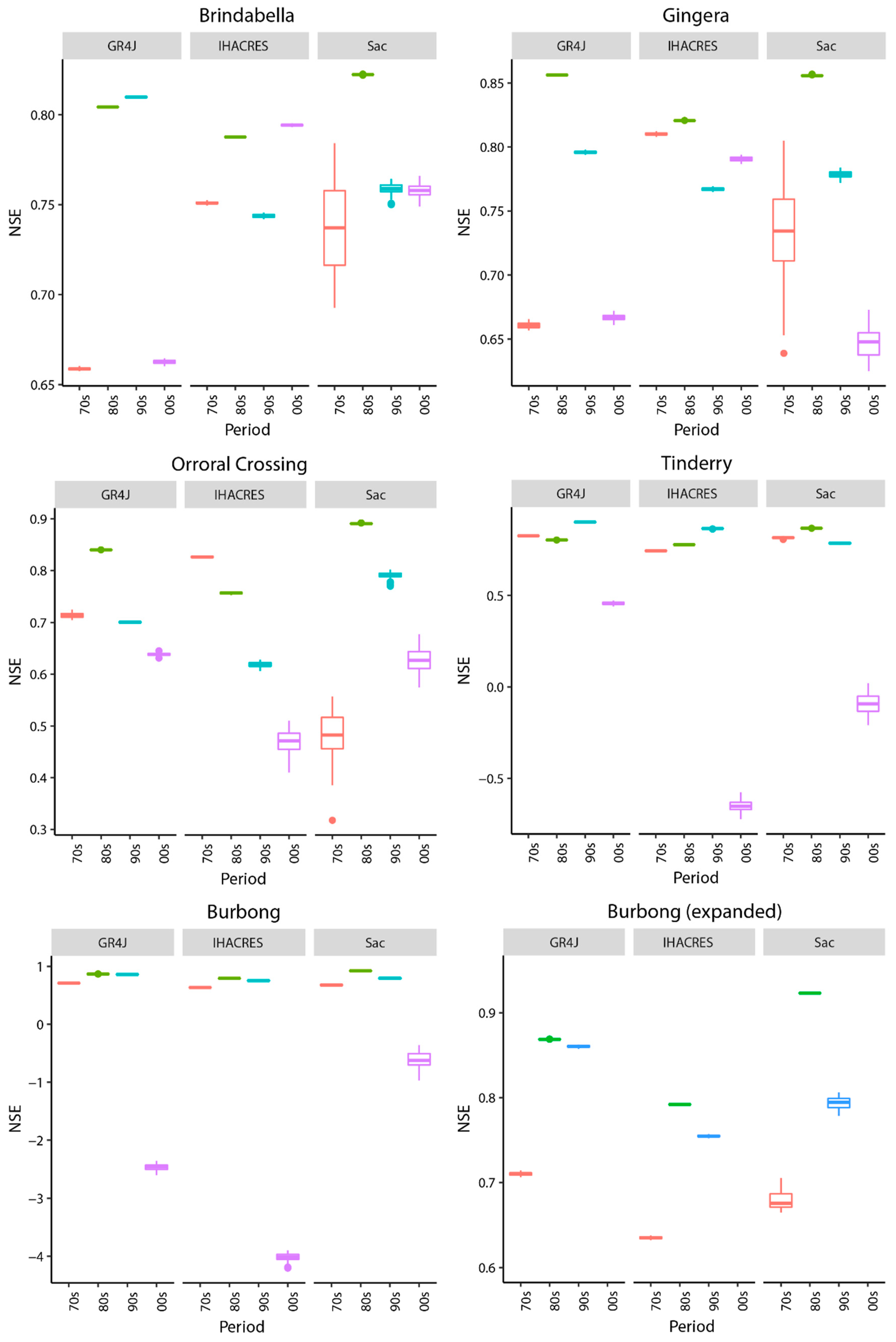
4.2. Investigation of the Distribution of Model Performance Values for Calibration and Validation Periods
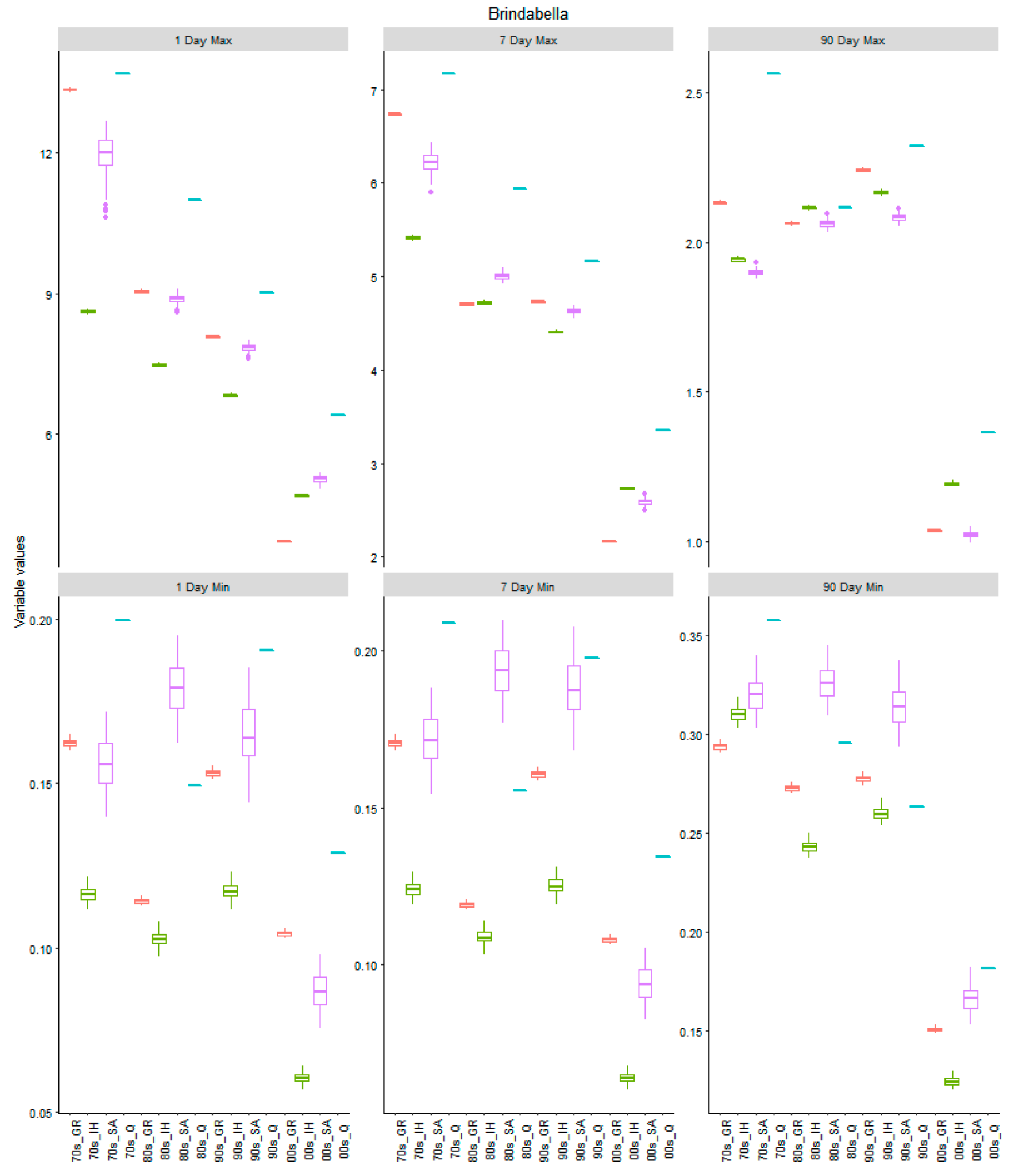
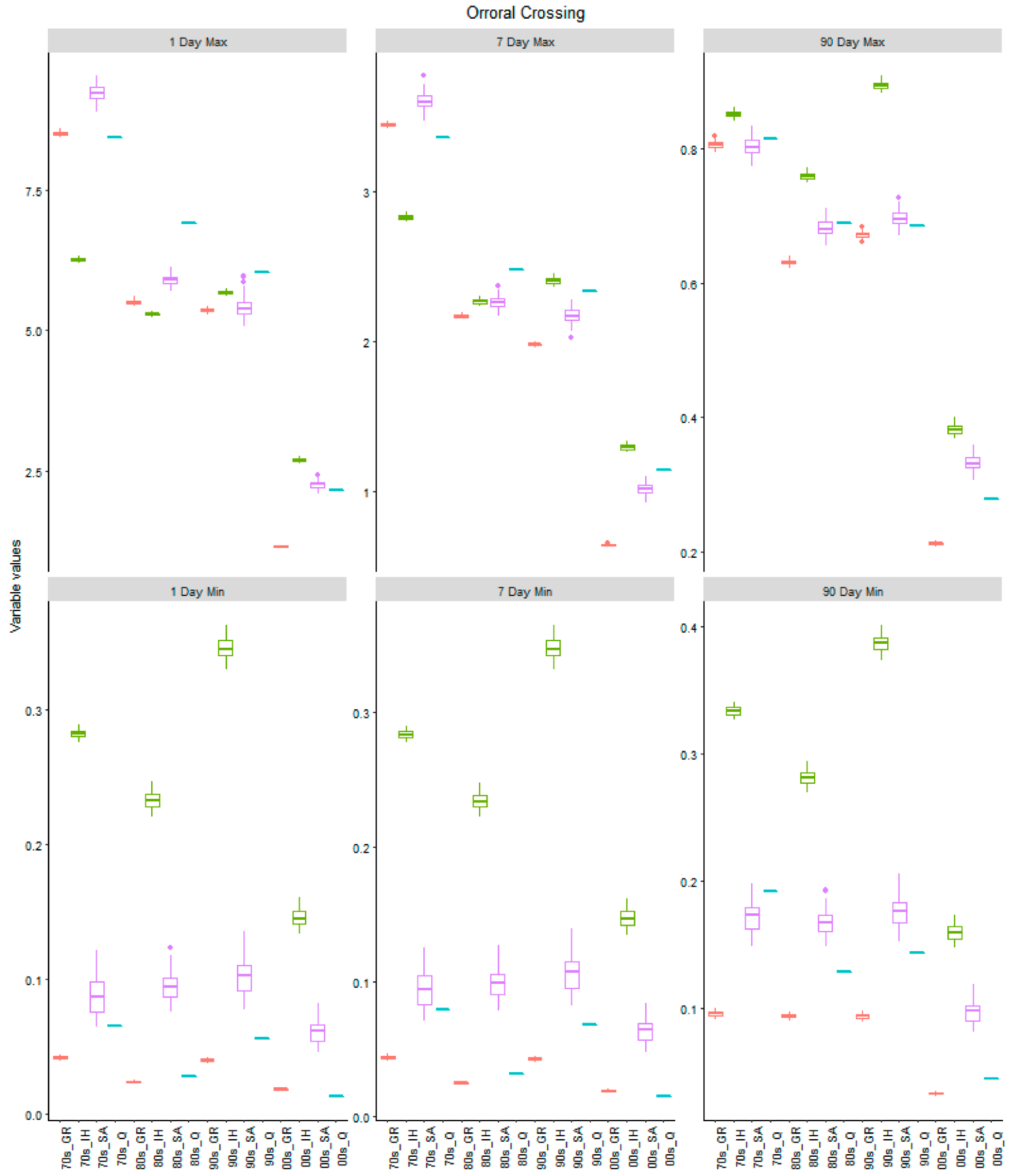
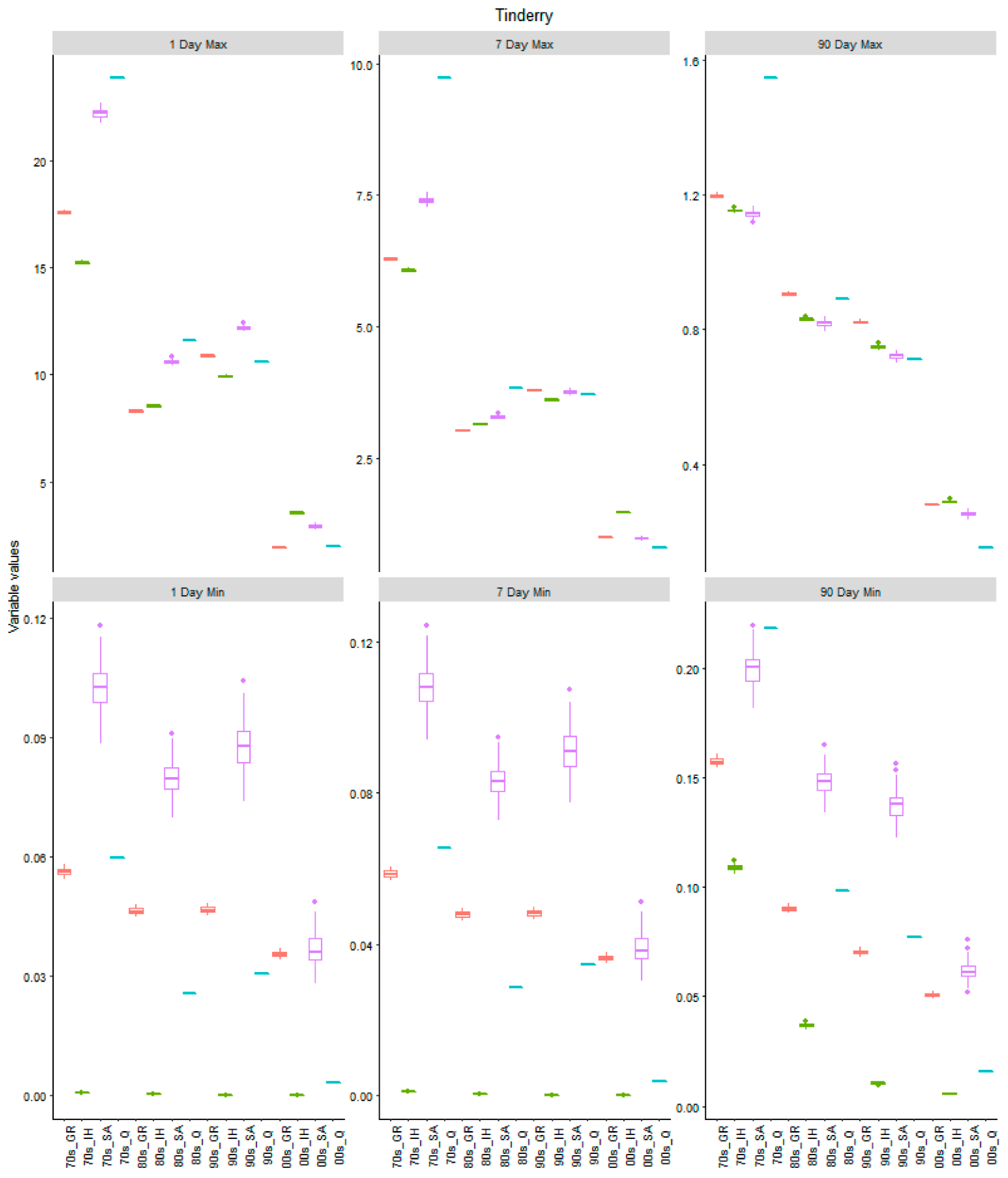
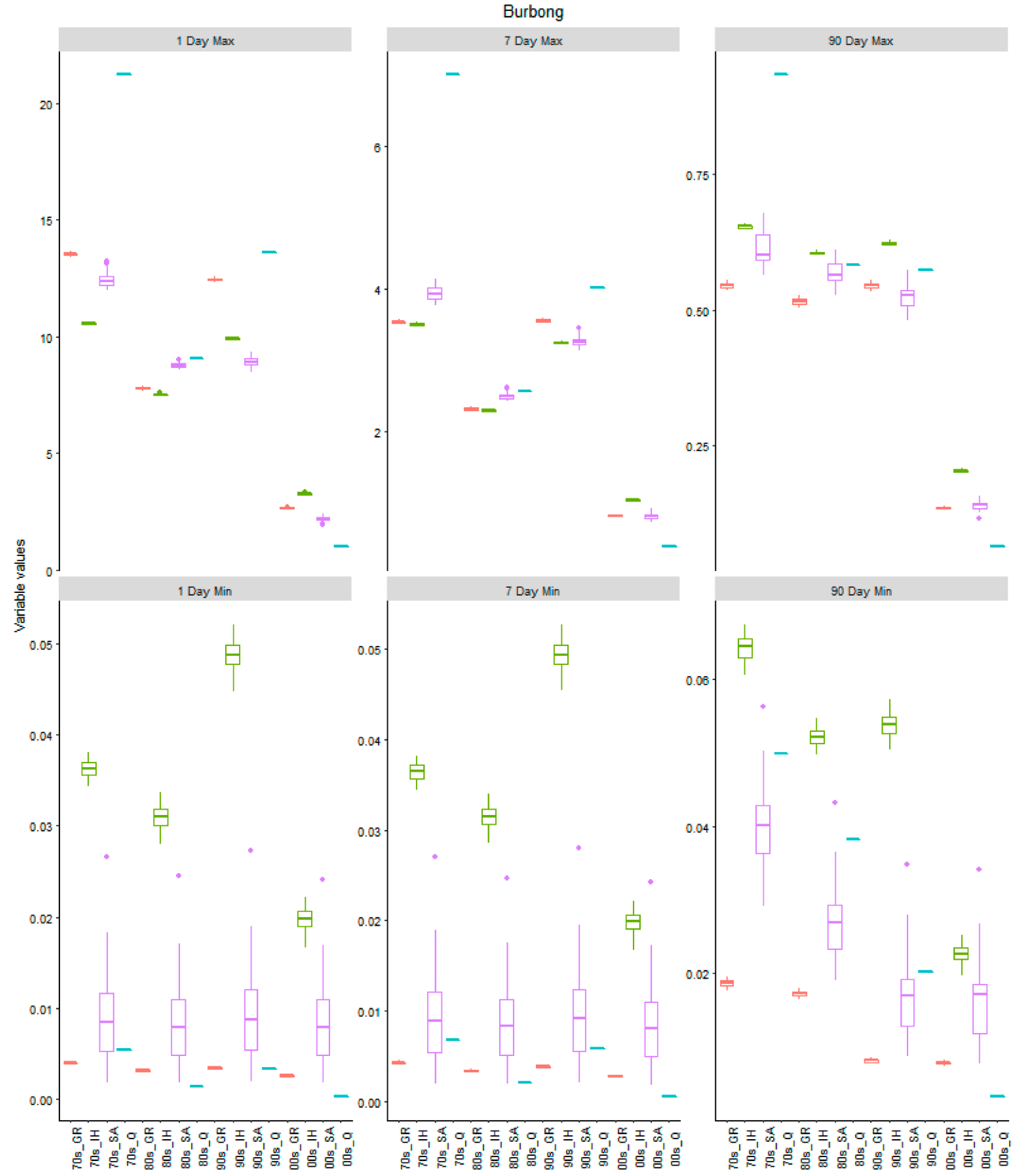
4.3. Investigation of the Distribution of Hydrologic Indicators for Calibration and Validation Periods
5. Conclusions
Author Contributions
Funding
Acknowledgments
Conflicts of Interest
References
- Shin, M.-J.; Guillaume, J.H.A.; Croke, B.F.W.; Jakeman, A.J. Addressing ten questions about conceptual rainfall-runoff models with global sensitivity analyses in R. J. Hydrol. 2013, 503, 135–152. [Google Scholar] [CrossRef]
- Clark, M.P.; Slater, A.G.; Rupp, D.E.; Woods, R.A.; Vrugt, J.A.; Gupta, H.V.; Wagener, T.; Hay, L.E. Framework for Understanding Structural Errors (FUSE): A modular framework to diagnose differences between hydrological models. Water Resour. Res. 2008, 44, W00B02. [Google Scholar] [CrossRef]
- Kavetski, D.; Kuczera, G.; Franks, S.W. Bayesian analysis of input uncertainty in hydrological modeling: 1. Theory. Water Resour. Res. 2006, 42, W03407. [Google Scholar] [CrossRef]
- Shin, M.-J.; Guillaume, J.H.A.; Croke, B.F.W.; Jakeman, A.J. A review of foundational methods for checking the structural identifiability of models: Results for rainfall-runoff. J. Hydrol. 2015, 520, 1–16. [Google Scholar] [CrossRef]
- Van Hoey, S.; Seuntjens, P.; van der Kwast, J.; Nopens, I. A qualitative model structure sensitivity analysis method to support model selection. J. Hydrol. 2014, 519, 3426–3435. [Google Scholar] [CrossRef]
- Massmann, C.; Holzmann, H. Analysing the Sub-processes of a Conceptual Rainfall-Runoff Model Using Information About the Parameter Sensitivity and Variance. Environ. Model. Assess. 2015, 20, 41–53. [Google Scholar] [CrossRef]
- Beven, K.; Freer, J. Equifinality, data assimilation, and uncertainty estimation in mechanistic modelling of complex environmental systems using the GLUE methodology. J. Hydrol. 2001, 249, 11–29. [Google Scholar] [CrossRef]
- Cho, H.; Park, J.; Kim, D. Evaluation of Four GLUE Likelihood Measures and Behavior of Large Parameter Samples in ISPSO-GLUE for TOPMODEL. Water 2019, 11, 447. [Google Scholar] [CrossRef]
- Wagener, T.; McIntyre, N.; Lees, M.J.; Wheater, H.S.; Gupta, H.V. Towards reduced uncertainty in conceptual rainfall-runoff modelling: Dynamic identifiability analysis. Hydrol. Process. 2003, 17, 455–476. [Google Scholar] [CrossRef]
- Vrugt, J.A.; Gupta, H.V.; Bouten, W.; Sorooshian, S. A Shuffled Complex Evolution Metropolis algorithm for optimization and uncertainty assessment of hydrologic model parameters. Water Resour. Res. 2003, 39, 1201. [Google Scholar] [CrossRef]
- Croke, B.F.W.; Jakeman, A.J. Predictions in catchment hydrology: An Australian perspective. Mar. Freshwater Res. 2001, 52, 65–79. [Google Scholar] [CrossRef]
- van Dijk, A.I.; Beck, H.E.; Crosbie, R.S.; Jeu, R.A.; Liu, Y.Y.; Podger, G.M.; Timbal, B.; Viney, N.R. The Millennium Drought in southeast Australia (2001–2009): Natural and human causes and implications for water resources, ecosystems, economy, and society. Water Resour. Res. 2013, 49, 1040–1057. [Google Scholar] [CrossRef]
- Anctil, F.; Perrin, C.; Andréassian, V. Impact of the length of observed records on the performance of ANN and of conceptual parsimonious rainfall-runoff forecasting models. Environ. Modell. Softw. 2004, 19, 357–368. [Google Scholar] [CrossRef]
- Kim, H.S.; Croke, B.F.W.; Jakeman, A.J.; Chiew, F.H.S. An assessment of modelling capacity to identify the impacts of climate variability on catchment hydrology. Math. Comput. Simulat. 2011, 81, 1419–1429. [Google Scholar] [CrossRef]
- Yapo, P.O.; Gupta, H.V.; Sorooshian, S. Automatic calibration of conceptual rainfall-runoff models: Sensitivity to calibration data. J. Hydrol. 1996, 181, 23–48. [Google Scholar] [CrossRef]
- Andréassian, V.; Lerat, J.; Le Moine, N.; Perrin, C. Neighbors: Nature’s own hydrological models. J. Hydrol. 2012, 414, 49–58. [Google Scholar] [CrossRef]
- Shin, M.-J.; Eum, H.-I.; Kim, C.-S.; Jung, I.-W. Alteration of hydrologic indicators for Korean catchments under CMIP5 climate projections. Hydrol. Process. 2016, 30, 4517–4542. [Google Scholar] [CrossRef]
- van Werkhoven, K.; Wagener, T.; Reed, P.; Tang, Y. Sensitivity-guided reduction of parametric dimensionality for multi-objective calibration of watershed models. Adv. Water Resour. 2009, 32, 1154–1169. [Google Scholar] [CrossRef]
- Perrin, C.; Michel, C.; Andréassian, V. Improvement of a parsimonious model for streamflow simulation. J. Hydrol. 2003, 279, 275–289. [Google Scholar] [CrossRef]
- Le Moine, N.; Andréassian, V.; Mathevet, T. Confronting surface- and groundwater balances on the La Rochefoucauld-Touvre karstic system (Charente, France). Water Resour. Res. 2008, 44, W03403. [Google Scholar] [CrossRef]
- Croke, B.F.W.; Jakeman, A.J. A catchment moisture deficit module for the IHACRES rainfall-runoff model. Environ. Modell. Softw. 2004, 19, 1–5. [Google Scholar] [CrossRef]
- Burnash, R.J.C.; Ferral, R.L.; McGuire, R.A. A Generalized Streamflow Simulation System: Conceptual Modeling for Digital Computers, Technical Report; U.S. National Weather Service: Sacramento, CA, USA, 1973. [Google Scholar]
- Podger, G (Cooperative Research Centre for Catchment Hydrology). Rainfall Runoff Library (RRL) User Guide. 2004. Available online: https://toolkit.ewater.org.au/Tools/RRL/documentation (accessed on 18 June 2004).
- Andrews, F.T.; Croke, B.F.W.; Jakeman, A.J. An open software environment for hydrological model assessment and development. Environ. Modell. Softw. 2011, 26, 1171–1185. [Google Scholar] [CrossRef]
- Vrugt, J.A.; ter Braak, C.J.F.; Diks, C.G.H.; Robinson, B.A.; Hyman, J.M.; Higdon, D. Accelerating Markov Chain Monte Carlo simulation by Differential Evolution with self-adaptive randomized subspace sampling. Int. J. Nonlin. Sci. Num. 2008, 10, 273–290. [Google Scholar] [CrossRef]
- Nash, J.E.; Sutcliffe, J.V. River flow forecasting through conceptual models part I—A discussion of principles. J. Hydrol. 1970, 10, 282–290. [Google Scholar] [CrossRef]
- Beven, K. Prophecy, reality and uncertainty in distributed hydrological modelling. Adv. Water Resour. 1993, 16, 41–51. [Google Scholar] [CrossRef]
- Beven, K. A manifesto for the equifinality thesis. J. Hydrol. 2006, 320, 18–36. [Google Scholar] [CrossRef]
- Indicators of Hydrologic Alteration Version 7.1: User’s Manual; The Nature Conservancy: Arlington, VA, USA, 2009.
- Richter, B.D.; Baumgartner, J.V.; Powell, J.; Braun, D.P. A method for assessing hydrologic alteration within ecosystems. Conserv. Biol. 1996, 10, 1163–1174. [Google Scholar] [CrossRef]
- Sanford, S.E.; Creed, I.F.; Tague, C.L.; Beall, F.D.; Buttle, J.M. Scale-dependence of natural variability of flow regimes in a forested landscape. Water Resour. Res. 2007, 43, W08414. [Google Scholar] [CrossRef]
- Monk, W.A.; Peters, D.L.; Baird, D.J. Assessment of ecologically relevant hydrological variables influencing a cold-region river and its delta: The Athabasca River and the Peace-Athabasca Delta, northwestern Canada. Hydrol. Process. 2012, 26, 1827–1839. [Google Scholar] [CrossRef]
- Shrestha, R.R.; Schnorbus, M.A.; Werner, A.T.; Zwiers, F.W. Evaluating Hydroclimatic Change Signals from Statistically and Dynamically Downscaled GCMs and Hydrologic Models. J. Hydrometeorol. 2014, 15, 844–860. [Google Scholar] [CrossRef]


| Parameter Name | Unit | Range | Description |
|---|---|---|---|
| GR4J | |||
| x1 | (mm) | 50–5000 | Maximum capacity of the production store |
| x2 | (mm) | (−15)–4 | Groundwater exchange coefficient |
| x3 | (mm) | 10–1300 | One day ahead maximum capacity of the routing store |
| x4 | (day) | 0.5–5 | Time base of Unit Hydrograph UH1 |
| IHACRES-CMD a | |||
| f | (-) | 0.5–1.3 | CMD stress threshold as a proportion of d |
| e | (-) | 1 (fixed) | Temperature to Potential Evapotranspiration (PET) conversion factor |
| d | (mm) | 200 (fixed) | CMD threshold for producing flow |
| τs (tau_s) | (day) | 10–1000 | Time constant for slow flow store |
| τq (tau_q) | (day) | 0–10 | Time constant for quick flow store |
| vs (v_s) | (-) | 0–1 | Fractional volume for slow flow |
| Sacramento | |||
| uztwm | (mm) | 1–150 | Upper zone tension water maximum capacity |
| uzfwm | (mm) | 1–150 | Upper zone free-water maximum capacity |
| uzk | (1/day) | 0.1–0.5 | Upper zone free-water lateral depletion rate |
| pctim | (-) | 0.000001–0.1 | Fraction of the impervious area |
| adimp | (-) | 0–0.4 | Fraction of the additional impervious area |
| zperc | (-) | 1–250 | Maximum percolation rate coefficient |
| rexp | (-) | 0–5 | Exponent of the percolation equation |
| lztwm | (mm) | 1–500 | Lower zone tension water maximum capacity |
| lzfsm | (mm) | 1–1000 | Lower zone supplementary free-water maximum capacity |
| lzfpm | (mm) | 1–1000 | Lower zone primary free-water maximum capacity |
| lzsk | (1/day) | 0.01–0.25 | Lower zone supplementary free-water depletion rate |
| lzpk | (1/day) | 0.0001–0.25 | Lower zone primary free-water depletion rate |
| pfree | (-) | 0–0.6 | Direct percolation fraction from upper to lower zone free-water storage |
| side | (-) | 0.0 (fixed) | Fraction of base flow that is draining to areas other than the observed channel |
| rserv | (-) | 0.3 (fixed) | Fraction of the lower zone free-water that is unavailable for transpiration purposes |
| riva | (-) | 0.0 (fixed) | Fraction of the riparian vegetation area |
| Catchment | Calibration | GR4J | IHACRES | Sacramento | |||||||||
|---|---|---|---|---|---|---|---|---|---|---|---|---|---|
| Diff_70s | Diff_80s | Diff_90s | Diff_00s | Diff_70s | Diff_80s | Diff_90s | Diff_00s | Diff_70s | Diff_80s | Diff_90s | Diff_00s | ||
| Brindabella | 1970s | 0.00003 | 0.00420 | 0.00627 | 0.00386 | 0.00002 | 0.00356 | 0.00707 | 0.00518 | 0.00023 | 0.01095 | 0.01716 | 0.01196 |
| Brindabella | 1980s | 0.00286 | 0.00002 | 0.00134 | 0.00434 | 0.00299 | 0.00004 | 0.00352 | 0.00211 | 0.09150 | 0.00057 | 0.01414 | 0.01708 |
| Brindabella | 1990s | 0.01189 | 0.00933 | 0.00033 | 0.01793 | 0.00481 | 0.00327 | 0.00005 | 0.00776 | 0.06583 | 0.05568 | 0.00272 | 0.03399 |
| Brindabella | 2000s | 0.00723 | 0.00987 | 0.00954 | 0.00007 | 0.00660 | 0.00299 | 0.00392 | 0.00012 | 0.26415 | 0.29611 | 0.09610 | 0.01273 |
| Gingera | 1970s | 0.00004 | 0.00560 | 0.00716 | 0.00731 | 0.00004 | 0.00493 | 0.01076 | 0.01675 | 0.00037 | 0.01295 | 0.02213 | 0.02654 |
| Gingera | 1980s | 0.00885 | 0.00009 | 0.00394 | 0.01104 | 0.00449 | 0.00008 | 0.00443 | 0.00725 | 0.16607 | 0.00153 | 0.01199 | 0.04793 |
| Gingera | 1990s | 0.00651 | 0.00257 | 0.00007 | 0.00918 | 0.00674 | 0.00373 | 0.00010 | 0.00334 | 0.22802 | 0.07705 | 0.00137 | 0.06841 |
| Gingera | 2000s | 0.02071 | 0.01922 | 0.02102 | 0.00014 | 0.01231 | 0.00624 | 0.00287 | 0.00031 | 0.84590 | 0.92870 | 0.54380 | 0.02767 |
| Orroral Crossing | 1970s | 0.00026 | 0.01215 | 0.01668 | 0.02329 | 0.00013 | 0.00714 | 0.01960 | 0.06613 | 0.00254 | 0.03060 | 0.33796 | 0.18626 |
| Orroral Crossing | 1980s | 0.02002 | 0.00015 | 0.00470 | 0.01395 | 0.00529 | 0.00667 | 0.02197 | 0.09985 | 0.23913 | 0.00191 | 0.03166 | 0.10289 |
| Orroral Crossing | 1990s | 0.00762 | 0.02289 | 0.00131 | 0.01618 | 0.00893 | 0.00672 | 0.00235 | 0.00616 | 0.57379 | 0.08821 | 0.00287 | 0.11608 |
| Orroral Crossing | 2000s | 0.11603 | 0.05491 | 0.04902 | 0.00436 | 0.02505 | 0.01708 | 0.01592 | 0.02056 | 2.09809 | 1.01582 | 1.64101 | 0.05611 |
| Tinderry | 1970s | 0.00001 | 0.00510 | 0.00853 | 0.11853 | 0.00001 | 0.00402 | 0.00564 | 0.10515 | 0.00012 | 0.01834 | 0.02443 | 0.43262 |
| Tinderry | 1980s | 0.00222 | 0.00003 | 0.00375 | 0.03209 | 0.00523 | 0.00007 | 0.00453 | 0.14629 | 0.01693 | 0.00040 | 0.01646 | 0.22845 |
| Tinderry | 1990s | 0.00364 | 0.00173 | 0.00008 | 0.03810 | 0.00510 | 0.00426 | 0.00008 | 0.08202 | 0.02236 | 0.01936 | 0.00055 | 0.16164 |
| Tinderry | 2000s | 0.04085 | 0.05561 | 0.05799 | 0.00176 | 0.03814 | 0.03267 | 0.03757 | 0.00397 | 0.21649 | 0.21524 | 0.17292 | 0.09934 |
| Burbong | 1970s | 0.00001 | 0.01606 | 0.01840 | 0.51824 | 0.00001 | 0.00866 | 0.01094 | 0.42153 | 0.00027 | 0.05746 | 0.04227 | 1.08569 |
| Burbong | 1980s | 0.00810 | 0.00010 | 0.00495 | 0.24704 | 0.00557 | 0.00024 | 0.00498 | 0.30410 | 0.04045 | 0.00080 | 0.02779 | 0.60965 |
| Burbong | 1990s | 0.00498 | 0.00279 | 0.00005 | 0.17522 | 0.00371 | 0.00124 | 0.00004 | 0.16237 | 0.03609 | 0.15757 | 0.02220 | 0.60478 |
| Burbong | 2000s | 0.03040 | 0.05012 | 0.04277 | 0.00493 | 0.03134 | 0.04194 | 0.03552 | 0.03896 | 0.32917 | 0.24963 | 0.05623 | 0.01174 |
| Catchment | Calibration | GR4J | IHACRES | Sacramento | |||||||||
|---|---|---|---|---|---|---|---|---|---|---|---|---|---|
| Max_70s | Max_80s | Max_90s | Max_00s | Max_70s | Max_80s | Max_90s | Max_00s | Max_70s | Max_80s | Max_90s | Max_00s | ||
| Brindabella | 1970s | 0.75 | 0.70 | 0.69 | 0.58 | 0.78 | 0.75 | 0.67 | 0.75 | 0.81 | 0.77 | 0.72 | 0.75 |
| Brindabella | 1980s | 0.66 | 0.80 | 0.81 | 0.66 | 0.75 | 0.79 | 0.75 | 0.80 | 0.78 | 0.82 | 0.76 | 0.77 |
| Brindabella | 1990s | 0.68 | 0.80 | 0.82 | 0.64 | 0.72 | 0.77 | 0.77 | 0.77 | 0.26 | 0.68 | 0.82 | 0.68 |
| Brindabella | 2000s | 0.57 | 0.67 | 0.67 | 0.78 | 0.74 | 0.78 | 0.75 | 0.80 | 0.29 | 0.53 | 0.70 | 0.79 |
| Gingera | 1970s | 0.78 | 0.74 | 0.69 | 0.54 | 0.84 | 0.79 | 0.69 | 0.70 | 0.86 | 0.80 | 0.73 | 0.71 |
| Gingera | 1980s | 0.67 | 0.86 | 0.80 | 0.67 | 0.81 | 0.82 | 0.77 | 0.79 | 0.80 | 0.86 | 0.78 | 0.67 |
| Gingera | 1990s | 0.68 | 0.85 | 0.81 | 0.62 | 0.78 | 0.81 | 0.78 | 0.81 | 0.79 | 0.83 | 0.79 | 0.69 |
| Gingera | 2000s | 0.40 | 0.69 | 0.57 | 0.79 | 0.79 | 0.81 | 0.78 | 0.82 | 0.43 | 0.81 | 0.78 | 0.81 |
| Orroral Crossing | 1970s | 0.87 | 0.78 | 0.72 | 0.70 | 0.85 | 0.74 | 0.60 | 0.47 | 0.93 | 0.84 | 0.76 | 0.50 |
| Orroral Crossing | 1980s | 0.72 | 0.84 | 0.70 | 0.65 | 0.83 | 0.76 | 0.63 | 0.51 | 0.56 | 0.89 | 0.80 | 0.68 |
| Orroral Crossing | 1990s | 0.85 | 0.76 | 0.76 | 0.69 | 0.82 | 0.75 | 0.68 | 0.70 | 0.37 | 0.88 | 0.83 | 0.69 |
| Orroral Crossing | 2000s | 0.66 | 0.75 | 0.64 | 0.81 | 0.78 | 0.73 | 0.67 | 0.71 | 0.70 | 0.77 | 0.75 | 0.79 |
| Tinderry | 1970s | 0.86 | 0.73 | 0.77 | −1.01 | 0.81 | 0.68 | 0.79 | −1.80 | 0.86 | 0.68 | 0.73 | −1.39 |
| Tinderry | 1980s | 0.83 | 0.80 | 0.90 | 0.47 | 0.75 | 0.78 | 0.87 | −0.58 | 0.82 | 0.87 | 0.79 | 0.02 |
| Tinderry | 1990s | 0.81 | 0.80 | 0.93 | 0.61 | 0.77 | 0.76 | 0.89 | 0.03 | 0.79 | 0.80 | 0.94 | 0.58 |
| Tinderry | 2000s | 0.73 | 0.72 | 0.87 | 0.78 | 0.52 | 0.60 | 0.67 | 0.76 | 0.83 | 0.77 | 0.84 | 0.74 |
| Burbong | 1970s | 0.85 | 0.42 | 0.28 | −21.3 | 0.75 | 0.54 | 0.50 | −17.3 | 0.90 | 0.05 | 0.65 | −0.72 |
| Burbong | 1980s | 0.71 | 0.87 | 0.86 | −2.36 | 0.64 | 0.79 | 0.76 | −3.90 | 0.71 | 0.92 | 0.81 | −0.36 |
| Burbong | 1990s | 0.71 | 0.86 | 0.88 | −2.17 | 0.68 | 0.77 | 0.79 | −3.51 | 0.82 | 0.85 | 0.88 | −0.33 |
| Burbong | 2000s | 0.44 | 0.61 | 0.53 | 0.86 | 0.28 | 0.45 | 0.40 | 0.78 | 0.70 | 0.59 | 0.56 | 0.76 |
© 2019 by the authors. Licensee MDPI, Basel, Switzerland. This article is an open access article distributed under the terms and conditions of the Creative Commons Attribution (CC BY) license (http://creativecommons.org/licenses/by/4.0/).
Share and Cite
Shin, M.-J.; Kim, C.-S. Analysis of the Effect of Uncertainty in Rainfall-Runoff Models on Simulation Results Using a Simple Uncertainty-Screening Method. Water 2019, 11, 1361. https://doi.org/10.3390/w11071361
Shin M-J, Kim C-S. Analysis of the Effect of Uncertainty in Rainfall-Runoff Models on Simulation Results Using a Simple Uncertainty-Screening Method. Water. 2019; 11(7):1361. https://doi.org/10.3390/w11071361
Chicago/Turabian StyleShin, Mun-Ju, and Chung-Soo Kim. 2019. "Analysis of the Effect of Uncertainty in Rainfall-Runoff Models on Simulation Results Using a Simple Uncertainty-Screening Method" Water 11, no. 7: 1361. https://doi.org/10.3390/w11071361
APA StyleShin, M.-J., & Kim, C.-S. (2019). Analysis of the Effect of Uncertainty in Rainfall-Runoff Models on Simulation Results Using a Simple Uncertainty-Screening Method. Water, 11(7), 1361. https://doi.org/10.3390/w11071361