A Census of the 1993–2016 Complex Mesoscale Eddy Processes in the South China Sea

Abstract

Mesoscale eddy process with at least one splitting and/or merging event can be defined as either a complex process or a simple process. Investigation of the difference between these two categories could provide new insights into how different factors, such as the seabed topography, Kuroshio intrusion, and winds, affect the origin, migration, and decay of the mesoscale eddies. This study compared the characteristics of the complex against the simple eddy processes in the South China Sea (SCS) from 1993 to 2016. We comprehensively analyzed the eddy processes with regards to their characteristic points, trajectories, and networks. The simple and complex processes share many similarities but do show significantly different behaviors. Both the simple and complex processes mainly start from the eastern SCS. However, the complex processes mainly vanish in the western SCS whereas the simple processes disappear almost everywhere across the SCS. The complex processes last longer and migrate more than the simple processes. Lastly, the complex processes mainly move westward within the community. The complex processes can be further categorized into complex anticyclonic and cyclonic eddy processes. Spatially, the splitting and merging events mainly occur in the southwest of Taiwan, northwest of the Luzon Island, and the southeast of Vietnam. Temporally, the merging and splitting events mainly occur in the fall. The interaction among the communities reveals the different migration patterns of the complex anticyclonic and cyclonic eddy processes in the SCS.

1. Introduction

Mesoscale eddies are a common dynamic phenomenon in the ocean, which is constantly moving around and changing with respect to their geometric and thematic characteristics. Previous studies have shown that mesoscale eddies migration facilitates transport and exchange of energy and substance in the oceans, and thus plays a significant role in the marine ecosystem, atmospheric environment, and surface ocean circulation [1,2,3,4,5]. Mesoscale eddies even show their effects on the migration and biogeochemical processes of the deep-ocean biological communities [3,4,5]. The heat exchange between the eddies and the atmosphere also affects the local wind field, clouds, and precipitation [6].

Many studies have been done on mesoscale eddies in different sea areas (such as the Pacific Ocean, the Indian Ocean, the Mediterranean Sea, Peru, etc.) to develop methods for identifying and tracking eddies [7,8,9], to examine eddies statistical characteristics [10,11,12,13,14,15] and the driving mechanisms behind them [16,17,18,19], and to study the influences of eddies on current circulation [2,20,21], oceanic ecology, and biogeochemical processes [5,22]. As in other waters, mesoscale eddies are also very common and active in the South China Sea (SCS), which is a marginal sea of the Pacific Ocean and also the largest semi-enclosed sea in the tropics. Different methods and multiple-source data sets have been used to examine the eddies in the SCS. For example, Yang et al. [23] and Yuan et al. [24] discovered a seasonal cyclonic (CE) and an anticyclonic eddy (AE) in the northern SCS from the climatological Levitus data and satellite altimeter data. From the Argo float data, Chow et al. [25] found perennial cold eddies in the south of the Dongsha Islands, mainly in winter or spring. Observational studies in the east of Vietnam [26] show that during the summer monsoon season, more anticyclonic eddies are found in the southern SCS whereas more cyclonic eddies are found in the northern SCS. Chen et al. [27] used in situ hydrographic data, 375 Argo profiles, and sea level anomaly (SLA) data to find relatively large current heat exchange both along the parallel and the meridian directions. Polar eddy current heat transfer was found in summer in the east of Vietnam. In the west of Luzon Island, polar heat exchange was found in winter. In the western Luzon Strait, a large equatorial heat transfer was found in winter.

Statistics has been widely used to depict the overall characteristics and movement patterns of the mesoscale eddies in different regions, from which efforts have been made to infer the driving mechanism and provide support for numerical simulation of the eddies [11,12,13,14,26]. Statistical analysis of the eddies in the SCS has been conducted from different perspectives by using the satellite altimeter data and observational data. Many studies focused on statistically analyzing the total number of eddies over a certain period and their lifespans, propagation directions, movement speeds, emerging and vanishing locales, spatiotemporal distribution patterns of their attributes, and even the correlation with the El Nino or La Nina events. For example, Wang et al. [11] examined the 1993 to 2000 sea surface height anomaly data and delineated the SCS into four regions based on the statistical analysis results of emerging locales of the eddies. By using the 1993 to 2001 TOPEX/Poseidon merged ERS-1/2 altimeter data, Lin et al. [26] showed that about 80% of eddies moved westward from the southwest of Taiwan to the east of southern Vietnam. Xiu et al. [12] conducted an eddy census in terms of the number, size, and lifespan from 1993 to 2007 and showed that the radius of the eddies ranged from 46.5 km to 223.5 km, with an average of 87.4 km. More than 70% of the eddies have a radius smaller than 100 km. They also found that the eddy activities in the SCS are not directly related to the El Niño–Southern Oscillation events. Chen et al. [13] examined the 1992 to 2009 SLA data and statistically summarized the seasonal and inter-annual variability of the eddies. They found that the eddies in the SCS mainly develop in an elongated northeast–southwest zone in the southwest of the Luzon Strait, and argued that eddy activity is sensitive to the wind stress curl in the northern SCS. Du et al. [14] investigated the general characteristics of the eddies in the SCS, particularly the spatial distribution patterns of eddy disappearing, reappearing, splitting, and merging activities.

Nowadays, mesoscale eddies are observed splitting and merging frequently thanks to the availability of high-quality spatial data, including satellite observation data, in situ observation data and the emergence of various model data [28,29,30,31,32]. In this study, we define a mesoscale eddy evolution process with at least one or without any splitting and merging event as a complex or simple process, respectively. It is valuable to study complex eddy processes as the splitting and merging events tend to impact seawater interaction and marine ecosystems more than the simple eddy processes [29,30]. For example, eddy splitting can cause eddy deformation, substance dispersion, and subsequent energy attenuation, affecting the temperature, salinity, water mass and microorganisms in the marine ecosystems [31]. Eddy merging may strengthen seawater interaction and the energy and entropy transfer across multiple scales in turbulent flows [29,32]. In fact, some studies have examined the complex processes and already recognized the great value of comparing simple against complex processes [28,29,30,31,32]. For example, Li et al. [31] argued that an eddy merging event may trigger a tropical storm, whereas a splitting event can initiate and enhance energy and material exchange among different regions. Not much statistical analysis has been conducted on the complex eddy processes in the SCS, and it remains unclear how the spatiotemporal characteristics are different between the simple and complex eddy processes.

Various factors, such as Kuroshio intrusion, wind stress, and coastal jet have been frequently cited to explain the origin, migration, and extinction of the eddies in the SCS. Unfortunately, the driving mechanism is still pretty vague. For example, the northern SCS is where eddies mainly start. It has been attributed to the shedding of the Kuroshio intrusion [24,33], wind stress [11,34] or influence of other eddies that invaded from the Pacific Ocean through the Luzon Strait [35]. In the east of Vietnam, the unstable strong currents along the coast may trigger more births of eddies [36]. A comprehensive statistical census of the complex eddies processes, in comparison with the simple processes, is thus needed and the results may shed new light on the mechanisms that drive the splitting, merging, and even the migration patterns of the eddies in the SCS.

This paper reports a comprehensive census of the complex eddy processes in the SCS from 1993 to 2016. The aim of this study is to examine the spatiotemporal characteristics of the complex eddy processes in the SCS to better understand their spatial distribution and mobility patterns in comparison with those of the simple processes. The movement patterns of eddy processes not only reflect their evolution characteristics but also imply the spatial interaction between the different geographic locations where the eddies pass. In this study, we used a variety of Geographic Information System (GIS)-based methods and network data mining method, including kernel density, hot spot analysis, and community detection, to examine the complex eddy processes.

The kernel density analysis calculates the density of point or linear features within a neighborhood around those features. The hot spot analysis identifies where features with either high or low values cluster spatially. Both kernel density and hot spot analysis are widely used in crime, utility, disease, rainfall, disasters, and wildlife mapping [37,38,39]. We applied these two methods to the SCS eddies to identify where the starting, demising, splitting, and merging locales are most clustered. Identifying the clustered locales would help us understand why certain locales are clustered at certain places. Community detection is an important method of network data mining, which is widely used to analyze the regional and mobile characteristics of objects such as mobile phone users and web graph in space [40,41]. The community detection method is used to delineate the SCS into different communities. We then examine the activities of the eddies within a community and between two adjacent communities to identify interaction among different communities (regions) in the SCS.

The paper is organized as follows. Section 2 introduces the data sets and methods used in this study. Section 3 focuses on the analysis results and we also compare and discuss the characteristics of the complex and simple eddy processes in the SCS. Section 4 focuses on the influence of topography on the splitting and merging of the complex eddy processes. Finally, we summarize this study and outline our future work in Section 4.2.

2. Data and Methods

2.1. Data

This study used the SLA data from January 1993 to December 2016. The SLA dataset is widely used in studying eddies [38] and has a temporal resolution of 1 day and a spatial resolution of ¼ degree [42]. We developed and improved the eddy identification and tracking methods and built a spatiotemporal database, from which every eddy in the SCS could be queried and studied for different purposes. In our dataset, there were 5773 eddy processes (3452 simple and 2321 complex processes). We provided a brief description of the data processing and data accuracy assessment results below. More details are available in Yi et al. [9,43,44,45].

The eddies in our database were identified using a hybrid detection (HD) method [43], which takes the advantages of the two widely-used eddy identification methods: the Okubo–Weiss (OW) [46,47] and the Sea Surface Height (SSH) [8] methods. An eddy truly exists only if it meets the OW criterion (W < −0.2σw, where σw is the spatial standard deviation of W, and W is computed from the horizontal velocity field as $\mathrm{W} ={ \mathrm{Sn}}^2+{\mathrm{Ss}}^2-\mathsf{\omega }$, where Sn, Ss, and ω are the straining deformation rate, the shearing deformation rate, and the vorticity, respectively) and includes either a local maximum or minimum SLA value. The identification results derived from the HD, OW, and SSH methods were compared, showing success rates of 96.6%, 96.6%, 100% and failure rates of 14.2%, 70.3%, 36.8%, respectively. Overall, the HD method outperformed the other two methods in correctly identifying eddies in the SCS [43].

The eddies identified were then concatenated using the method proposed by Yi et al. [44]. It is very common that an eddy is concatenated to a wrong predecessor or successor, particularly when an eddy splits, merges, disappears, and reappears. A global nearest neighbor filter (GNNF) approach [44], which combines the Kalman filter and optimal data association technologies to recursively recover the predecessor and successor of a specific eddy. The GNNF tracking results of the eddies in the SCS were compared with those derived from the distance-based search [48] and the overlap-based search [49] methods. The mismatching rates were 0.19%, 0.30% and 1.17% for these three methods respectively. The three methods were also used to track synthetic eddy trajectories with mismatching rates 0.2%, 0.4% and 0.5%, respectively. The comparison shows that the GNNF approach had its advantages in concatenating eddies.

2.2. Methods

In this study, an eddy process is represented as a trajectory with multiple points in chronological order (p1, p2, p3…… pn). Every point along the trajectory was defined with its longitude, latitude, and a timestamp (pi = (xi, yi, ti)). The trajectory could bear with or without branches. A structure containing no branches would represent a simple eddy process and otherwise a complex process (Figure 1). Any branch along the trajectory would represent either a splitting or a merging event.

The complexity of a trajectory was first quantitatively measured by a complexity index η (0 < η ≤ 1), which is the ratio between the number of the points along the branch(es) and all points on the trajectory. Figure 1a illustrates a complex trajectory. At a specific time-stamp, the eddy represented by point p3 splits into two eddies p4 and p5, which then merge into eddy p7. At another time-stamp, eddies p8 and p9 merge into eddy p10, which then splits into eddies p11 and p12. The total number of points along this trajectory is 13 and nine of them are on the branches. Therefore, the η is 0.69. A simple eddy trajectory (Figure 1b) is a linear structure without any branches thus has a complexity index 0 (η = 0).

In this study, conceptually the eddy trajectories could be represented as different objects: feature points, lines, and then networks. A variety of methods were used to statistically examine these objects (Figure 2). We first conducted kernel density and hot spot analysis on the feature points. Then we used a series of activity parameters to describe the movement characteristics of the feature points. The networks, formed by the points and lines, were examined using the fast folder community detection method [41]. 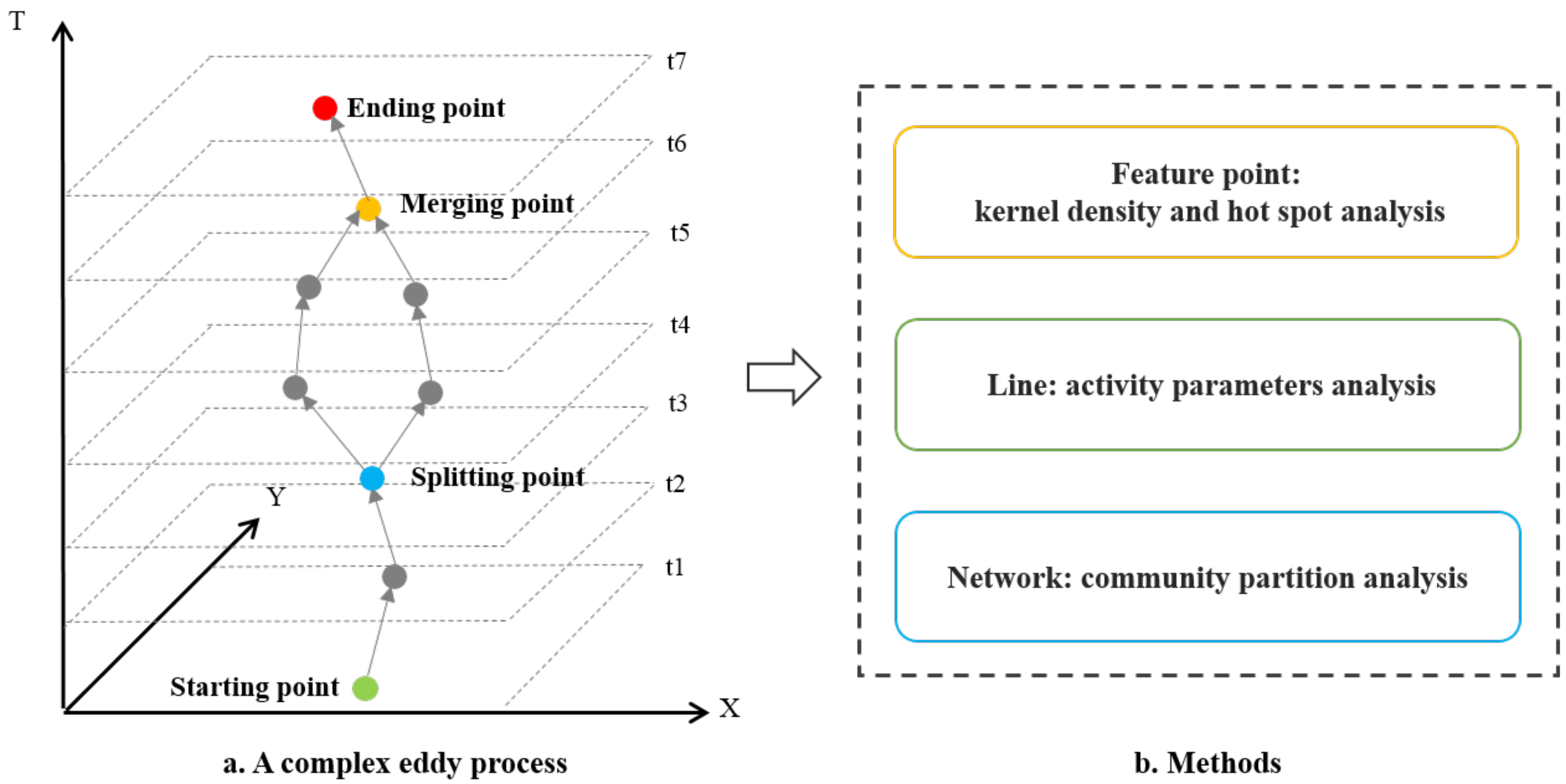The sections to follow provide more details about these methods.

2.2.1. Kernel Density and Hot Spot Analysis

We first conducted spatial kernel density and hot spot analysis on the feature points, which include the starting, ending, splitting, and merging points along the trajectories of cyclonic and anticyclonic eddies. Kernel density shows the concentration of points over an interpolated and smooth surface. In the places where points are clustered, the surface would have a higher density, which then gradually diminishes with increasing distance from the point clusters. The kernel density of the starting and ending points showed the places where eddies mainly originated and disappeared. By contrast, the kernel density of the splitting and merging points revealed the locales where the eddies tended to split and merge, probably due to the influence of different ocean environmental and climatic factors.

The Gi* method [50] was used to identify the hot and cold spots of the feature points by examining the z-score and p-value. A hot spot is a place where high-value features are surrounded by other high-value features. By contrast, a cold spot is a place where low-value features are clustered together. First, a 1° × 1° square fishnet was generated to cover the whole study area. We chose the 1° × 1° grid (about 108 km × 108 km in the SCS) as the radii of most eddies in the SCS are between 100 km and 200 km, and the average moving distance is 74 km [12,14]. Secondly, we counted the total number of every type of feature points in each grid. The counts and the Euclidean distance among the points were then used to calculate the Gi* values. Lastly, statistical significance was evaluated by looking at the z-score, p-value, and confidence level. A hot spot was identified when a z-score was greater than 1.65 and a p-value less than 0.10. In contrast, a low negative z-score (<−1.65) and a small p-value (<0.10) indicated a cold spot clustering, i.e., few eddies nearby.

2.2.2. Eddy Mobility Index

Activity space in geography is mainly used to examine human activities within a space [51,52]. We employed the same idea and computed four indexes, namely the complexity, activity duration, activity scope, and the number of activity points, to study how an eddy migrates within an activity space. The complexity, as discussed in Section 2.2, showed how complex an eddy trajectory is. The activity duration referred to the lifespan of an eddy, indicating how long an eddy process lasted. The activity scope was defined as the maximum distance between any two points along a specific track, indicating the maximum span within which an eddy was moving around. The number of activity points was the number of different positions that an eddy may occupy over its life span. More activity points suggested a more active eddy process.

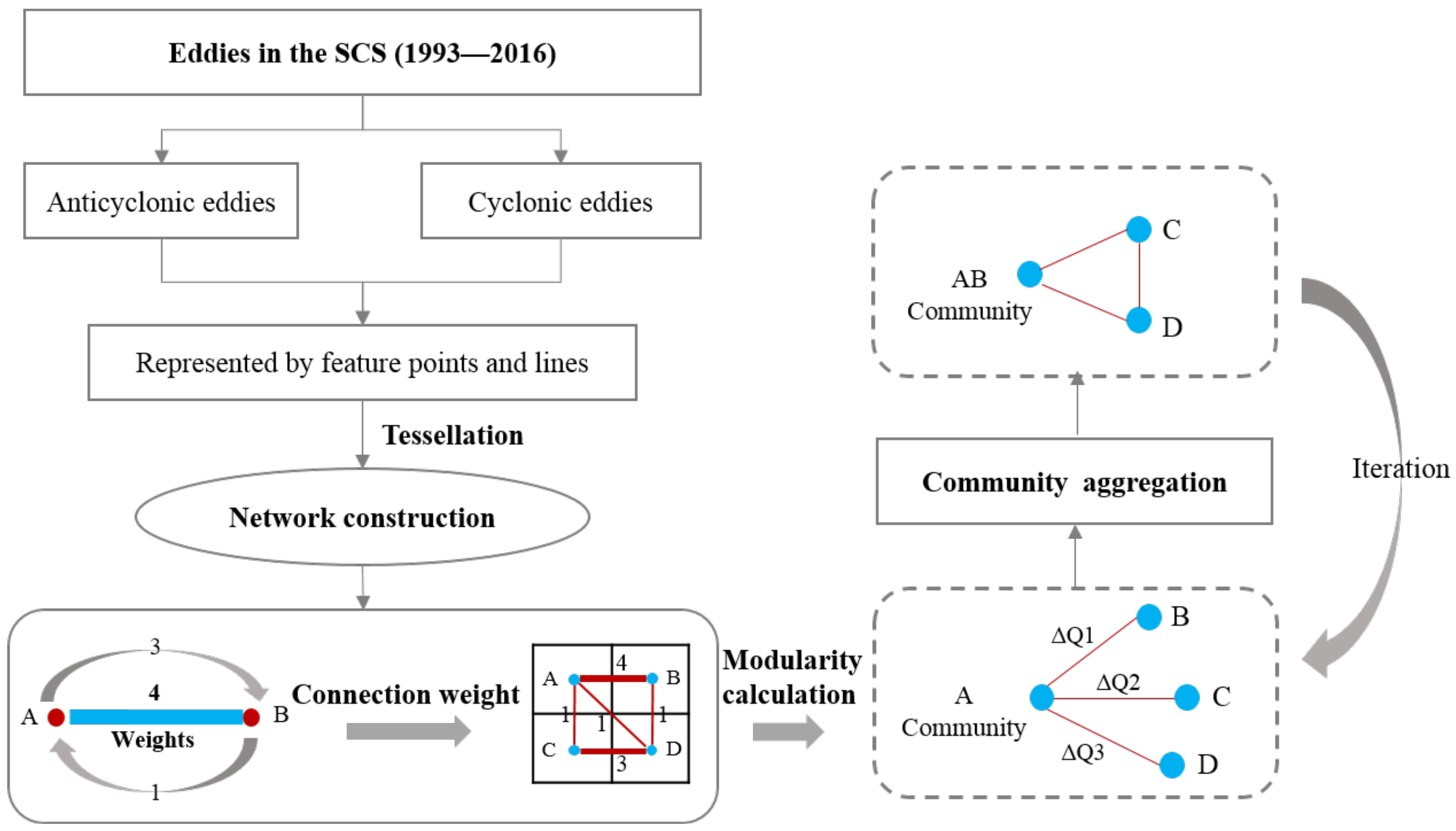
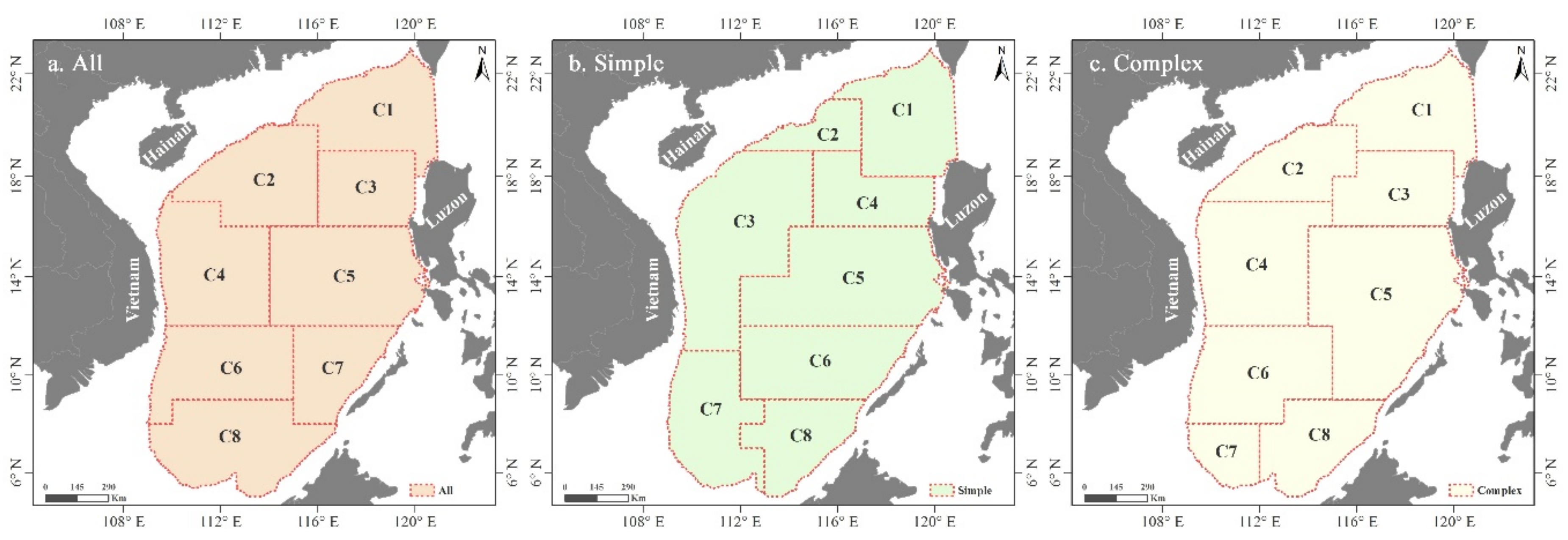
2.2.3. Community Detection

A geographic area could be delineated into a set of communities, each of which has similar attributes and/or functions in a network graph [53]. Many partitioning methods have been developed for community detection. This study used the fast unfolding method [54]. Eddy movement essentially is inhomogeneous as eddies are more active in certain regions across the SCS [13]. From a GIS perspective, any movement from one position to another could be represented as a connection (i.e., an edge). Movements of a large number of eddies could be translated and represented as a complex network consisting of nodes and edges. The network could then be delineated into different communities (Figure 3). Within a specific community, the eddies were similar in terms of their characteristics. The eddies’ characteristics showed homogeneity within a community but heterogeneity among communities.

The fast unfolding method includes two major steps in a sequence (Figure 3). The first step is to construct the movement network. We generated tessellated square grids of 1° × 1° to cover the whole study area and the center of each grid was represented as a node. We then counted the total number of eddies within each grid (node), respectively. The connections between any two adjacent grid nodes in the network were weighted using the total number of eddies that crossed their boundary. A network thus was constructed with the nodes representing the grids and edges the total number of eddies that crossed the boundary of two adjacent grids.

The second step was to partition the communities. Each node was regarded as a community and would be grouped with its neighboring nodes (communities) one by one. A modularity gain ∆Q was calculated as below [41].

$$\Delta \mathrm{Q} = \left[\frac{{{\displaystyle \sum }}_{\mathrm{in}}+{\mathrm{k}}_{\mathrm{i},\mathrm{in}}}{2\mathrm{m}}-{\left(\frac{{{\displaystyle \sum }}_{\mathrm{tot}}+{\mathrm{k}}_{\mathrm{i}}}{2\mathrm{m}}\right)}^2\right]-\left[\frac{{{\displaystyle \sum }}_{\mathrm{in}} }{2\mathrm{m}}-{\left(\frac{{{\displaystyle \sum }}_{\mathrm{tot}} }{2\mathrm{m}}\right)}^2-{\left(\frac{{\mathrm{k}}_{\mathrm{i}}}{2\mathrm{m}}\right)}^2\right]$$

(1)

where m represents the total connection weights across the entire network, ∑_in is the total connection weights within a specific community, ∑_tot is the sum of all connection weights associated with nodes within the specific community, k_i is the sum of the weights of all the connections to node i, k_{i, in} denotes the sum of the connection weights between nodes i and all the other nodes in the community. If the maximum ∆Q was greater than 0, the node would be grouped with its neighboring node. Otherwise, it stayed as it was. If a node was grouped into another community, a new network was constructed and the afore-mentioned procedure was repeated until no more nodes shifted to another community.

3. Results and Analysis

Over the study period from 1993 to 2016, 5773 tracks were identified and stored in our database. Among them, 2321 and 3452 were complex and simple eddy processes, respectively. The 2321 complex processes included 1120 and 1201 anticyclonic eddies (CPAEs) and cyclonic eddies (CPCEs), respectively. By contrast, 1682 and 1770 out of the 3452 simple processes were anticyclonic eddies (SPAEs) and cyclonic eddies (SPCEs), respectively.

3.1. Feature Points Analysis

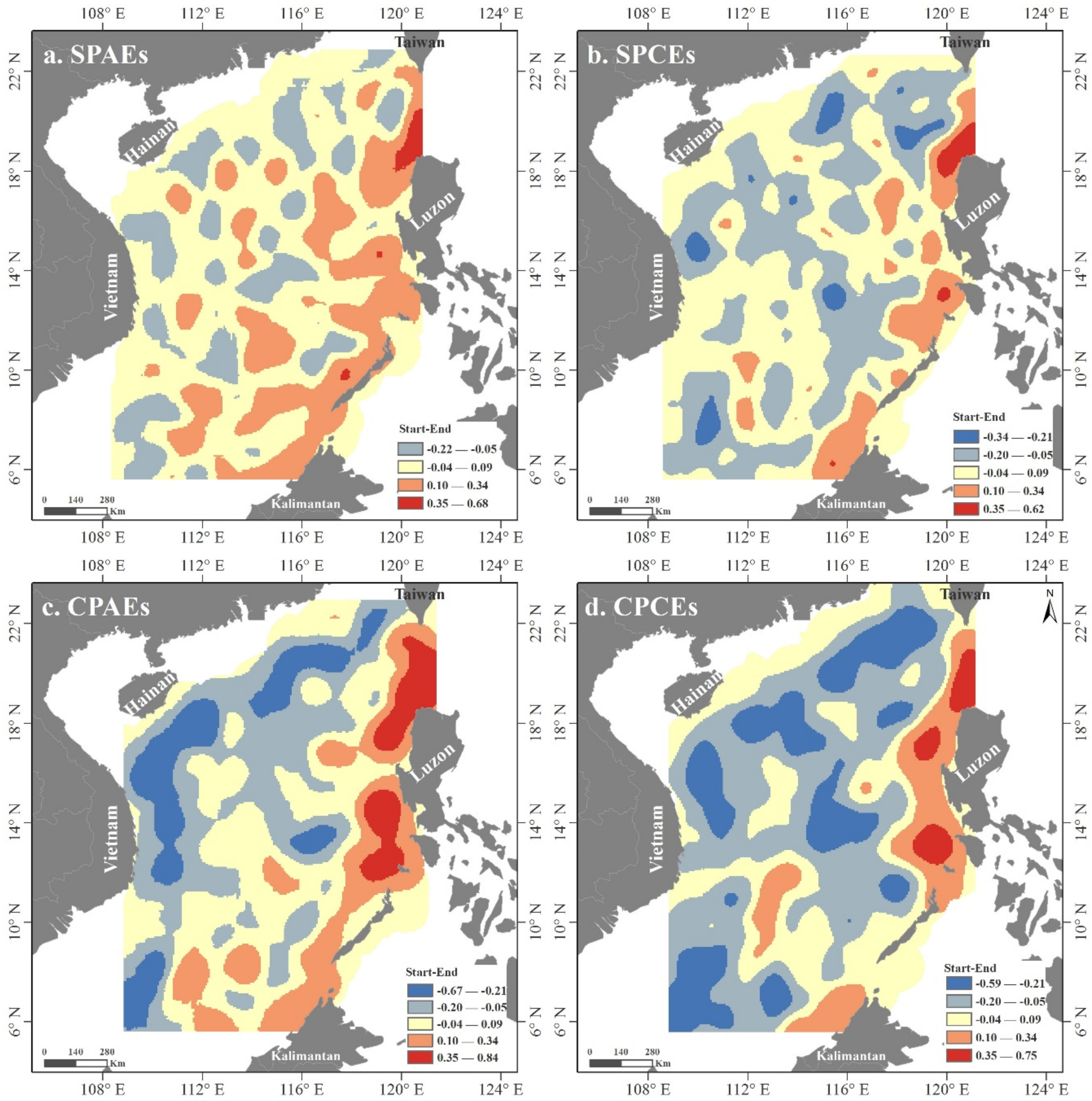
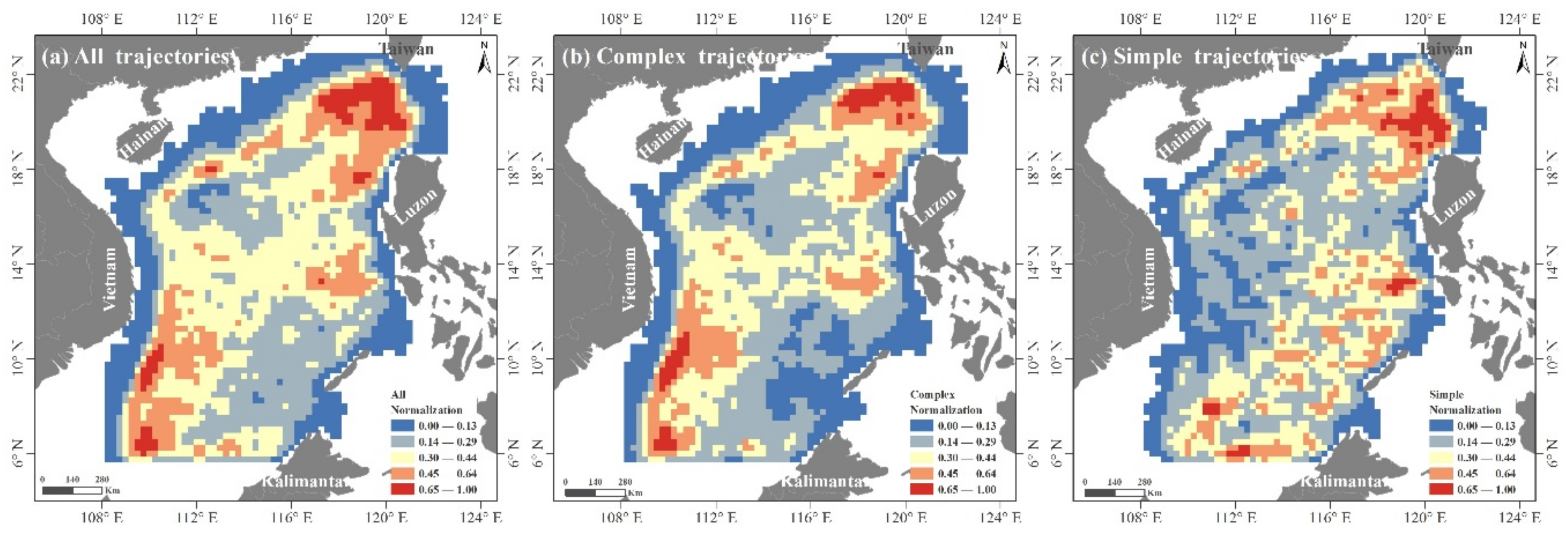
3.1.1. Kernel Density Analysis of the Simple and Complex Eddy Processes

The kernel density difference of the starting and ending points of the SPAEs (Figure 4a) and SPCEs (Figure 4b) showed that the eastern SCS witnesses more births than deaths of SPAEs and SPCEs, respectively. The death places of SPAEs and SPCEs were scattered across the whole SCS.

The kernel density difference of the starting and ending points of the CPAEs (Figure 4c) and CPCEs (Figure 4d) showed that more CPAEs and CPCEs were born in the eastern SCS and disappeared mainly in the western SCS. Such a finding is consistent with previous studies conducted by Wang et al. [11], Xiu et al. [12], and Chen et al. [13], in which the simple and complex eddy processes were not differentiated and studied as a whole. In this study, we examined the simple and complex eddy processes separately and found that the complex processes mainly disappeared in the western SCS whereas the simple processes disappeared almost everywhere across the SCS.

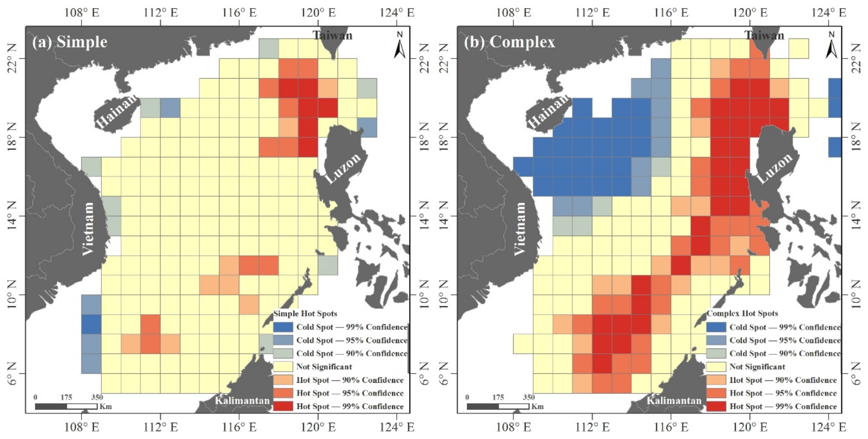
3.1.2. Hot Spot Analysis of Simple and Complex Eddy Processes

Figure 5 shows the hot and cold spots of where the simple and complex eddy processes originated, respectively. The hot spots were mainly located in the eastern SCS whereas the cold spots were mainly located in the western SCS. Such a pattern indicates that the eastern SCS was where most eddies start from. However, the hot spots of the complex eddy processes were more extensive and continuous in the eastern SCS, covering the area from the southwest of Taiwan, west of Luzon Strait and Luzon, Huangyan Island, Nansha Islands, northwest of the Kalimantan. By contrast, the hot spots of simple eddy processes were more isolated in the eastern SCS and could only be found in the southwest and northwest of Luzon and Palawan, southwest of Nansha Islands (7° N–9° N, 110° E–113° E). The same pattern was also found for the cold spots. Extensive cold spots were found for the complex eddy processes in the northwestern SCS. The cold spots of simple eddy processes were isolated and found in only a couple of grids in the east of Hainan Island and the southwestern SCS.

The difference between the hot and cold spots of the simple and complex eddy processes indicates that the complex processes originated from an extensive area in the eastern SCS. Very few complex eddy processes started from a quite extensive area in the northwestern SCS. By contrast, the simple processes mainly originated from three concentrated regions in the eastern SCS as shown in Figure 5a. There are only a couple of places in the western SCS that few simple processes originated from.

Both the kernel density and hot spot analysis indicated that the southwest of Taiwan Island, the west of Luzon Strait (Luzon strait between Taiwan Island and the Luzon Island) and the northwest of Luzon Island were where significant numbers of simple and complex processes started. Previous studies have shown that the local wind stress curl and Kuroshio intrusion contributed to the generation of both cyclonic and anticyclonic eddies in this area [33,55]. This study shows that origination of complex processes in this region could also be attributed to the local wind stress curl and Kuroshio intrusion. In Section 4.1.1, we discussed and analyzed how wind stress curl and Kuroshio intrusion affect the eddy evolution processes.

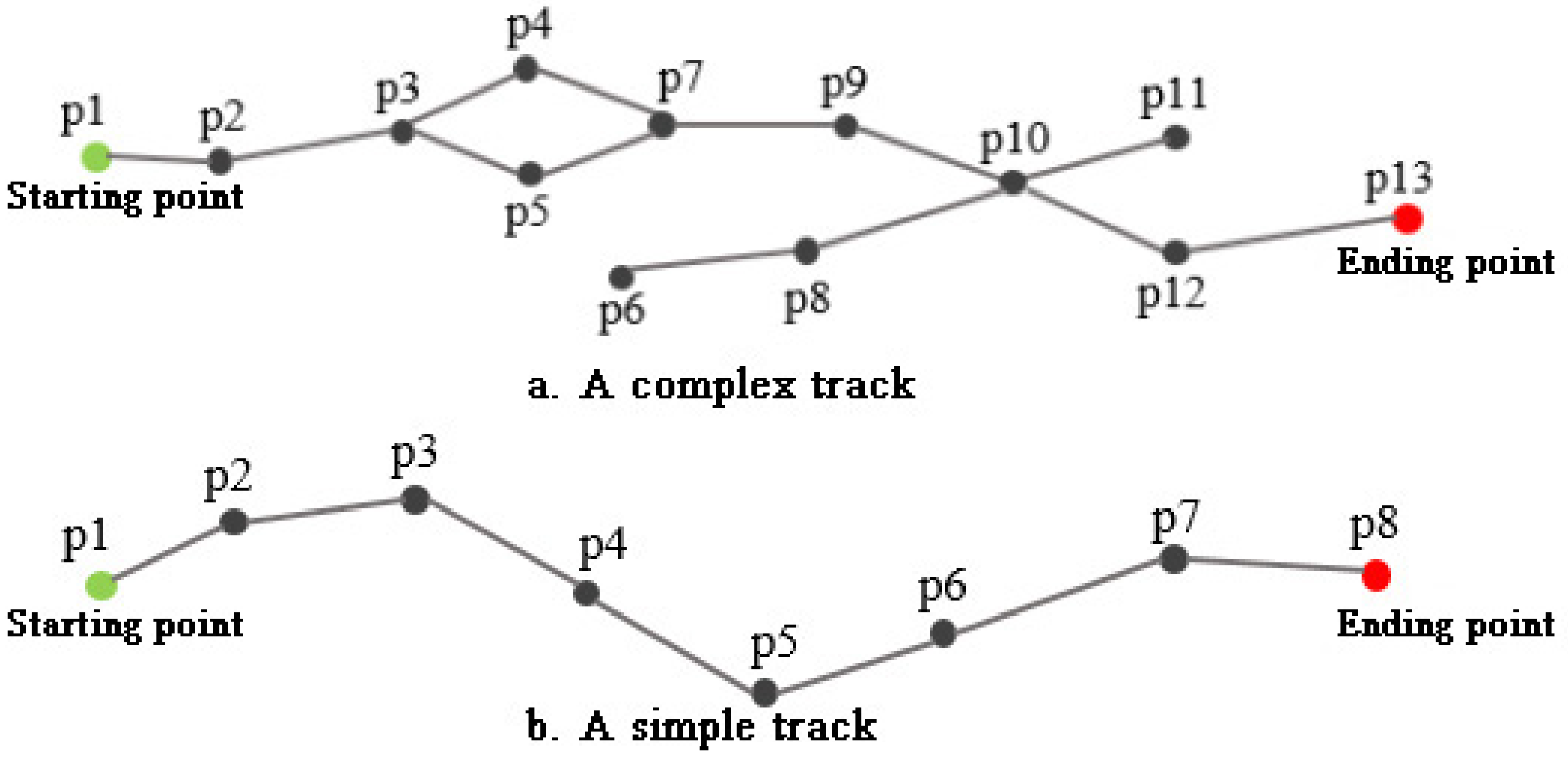
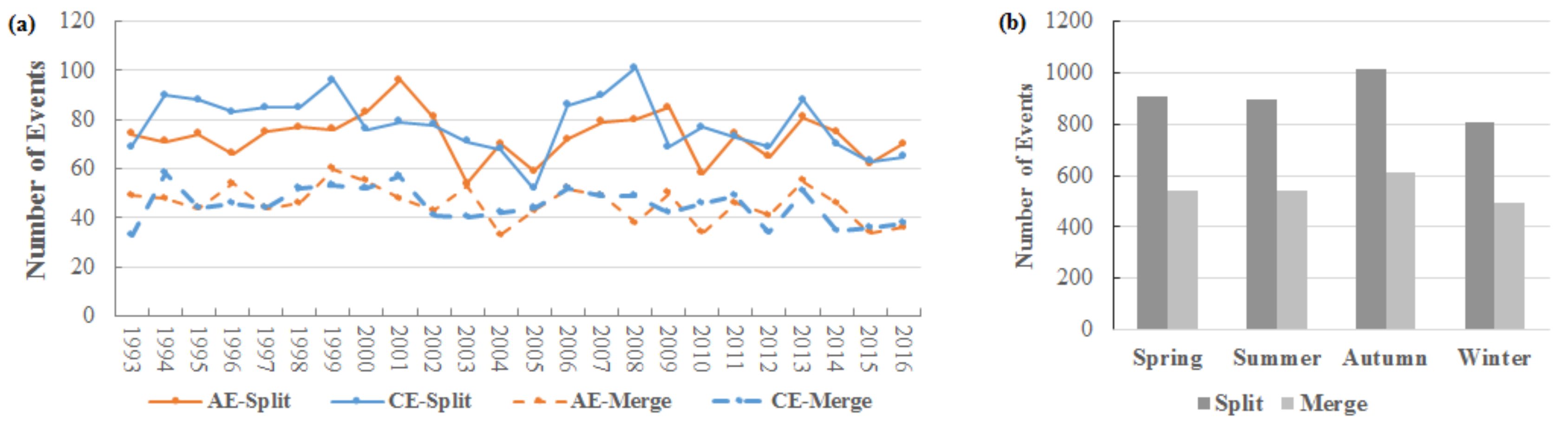
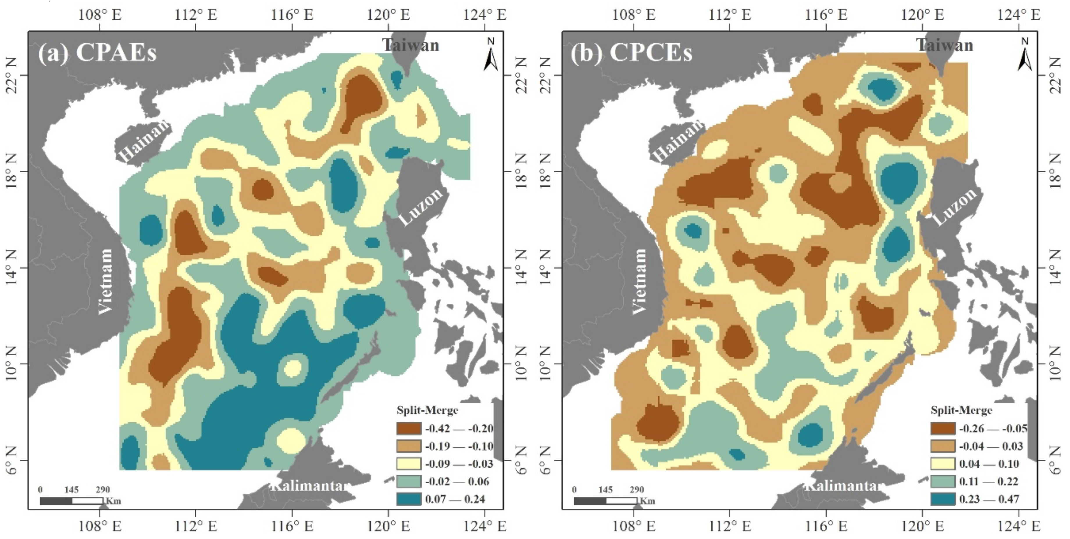
3.1.3. Splitting and Merging of Complex Eddy Processes

Unlike the simple eddy processes, the complex eddy processes split and merge. On average, the complex eddy processes split and merged 75 and 45 times every year in the SCS (Figure 6a). The CPAEs and CPCEs showed no significant difference between the numbers of merging and splitting events (Figure 6a). However, the numbers of splitting and merging events varied significantly in different seasons, with 908 (542), 898 (539), 1013 (612), and 809 (495) splitting (merging) events occurring in the spring, summer, fall, and winter, respectively (Figure 6b). Fall was the most favorable season that the complex eddy processes tended to split and merge.

The kernel density difference between the splitting and merging feature points shows that CPAEs merged more in the southwest of the Taiwan Island and the east of Vietnam, whereas they split more in the southeastern SCS (Figure 7a). By contrast, the CPCEs split more in the east of Luzon Island and the southwest of Taiwan Island (Figure 7b). In the southern SCS, the CPCEs split more except southeast of Vietnam. These regions were also where the eddies were concentrated, the differences in splitting/merging events between different areas will be discussed in Section 4.1.2.

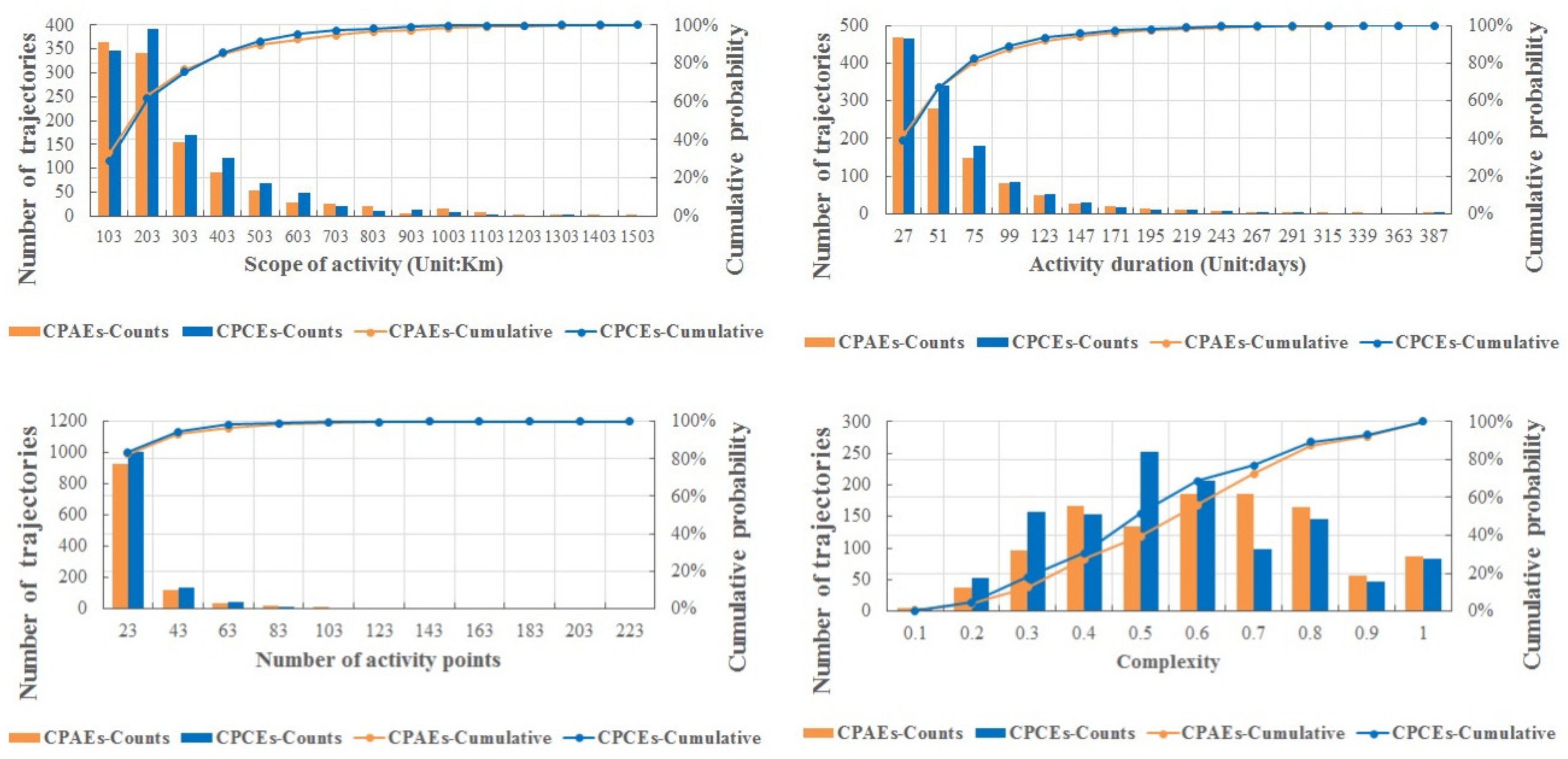
3.2. Line Analysis

Figure 8 shows the trajectory density of all (a), complex (b), and simple eddy processes (c) in the SCS, respectively. There was no significant difference between the trajectory distribution of all and complex processes, with higher density in the southwest of Taiwan and northwest of Luzon, west of Mindoro, and east and south of Vietnam. The trajectories of simple processes also concentrated in the southwest of Taiwan and northwest of Luzon. However, more trajectories of simple processes were found across an extensive region in the southwestern SCS.

The simple and complex eddy processes were also different in terms of the mobility indexes, including the activity duration, activity scope, and the number of activity points (

Table 1. Comparison of the means between the simple and complex eddy processes. The last column shows the significance test results of the Mann–Whitney U test for the mobility indexes.

Mobility Indexes	Simple Processes	Complex Processes	Sig.
Activity duration (days)	8	35	0.000
Scope of activity (km)	71.36	224.3	0.000
Number of activity points	5	16	0.000

). The complex eddy processes had a much longer activity duration (33.5 days) than that of the simple eddy processes (8 days). Both the activity scope and the number of activity points were over three times more extensive than those of the simple eddy processes. About 90% of the simple eddy processes have less than 10 active points and the travel range was less than 150 km in a lifespan less than 28 days (Figure 9). By contrast, about 90% of complex eddy processes had less than 43 active points and the travel range was less than 503 km in a lifespan less than 123 days. More than 80% of the complex eddy processes had a complexity index between 0.3 and 0.8 and the complexity index of the simple eddy processes, of course, was 0. All the differences between the means of all three mobility indexes were statistically significant (Table 1). However, there was no significant difference between the mobility indexes of the SPAEs and SPCEs. There were significantly more CPCEs than CPAEs with a complex index of 0.5 (Figure 9).

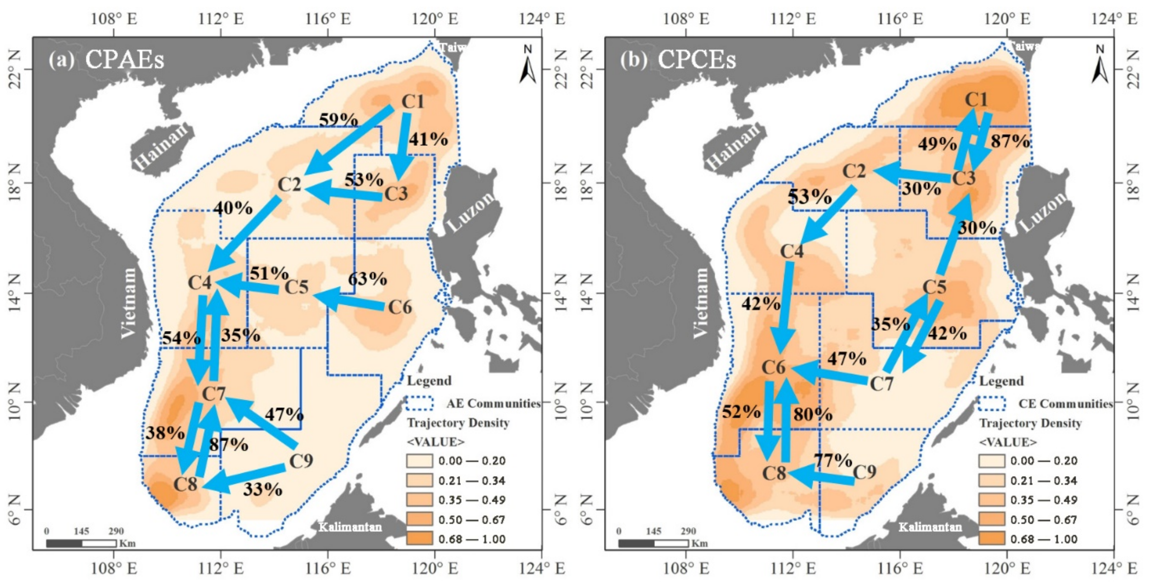
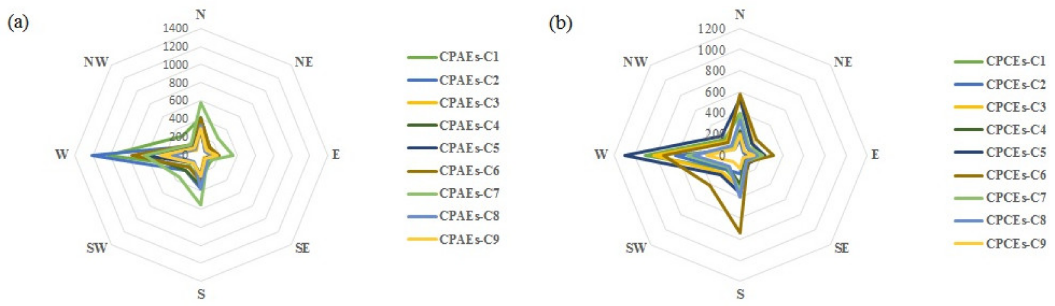
3.3. Network Analysis

The SCS beyond the 200-m bathymetry contour line could be divided into eight communities based on the networks built from all, simple, and complex eddy processes, respectively (Figure 10). The communities were roughly similar. Particularly, the community delineation results based on the complex- and all-eddy networks were very similar (Figure 10a,c). Roughly, the northern, central, and southern SCS could be divided into three, two, and three communities, respectively. However, difference does exist. For example, only one community was partitioned from the all-eddy networks in the southern part of the southern SCS (C8 in Figure 10a), whereas this region was divided into two simple- and complex-eddy communities, separately. A community was identified in the east of Hainan Island and Vietnam based on the simple-eddy networks (C3 in Figure 10c). This region was divided into two communities based on the complex- and all-eddy networks.

We then mainly focused on discussing how the SCS could be divided into different communities based on the networks constructed with the CPAEs (complex processes of anticyclonic eddies) and CPCEs (complex processes of cyclonic eddies) separately. The delineation results were very similar for the northern and southern SCS (Figure 11) but not for the central SCS. For example, the communities could be delineated for the central SCS based on the complex anticyclonic eddy networks (C4–C6 in the Figure 11a). However, no such communities were identified in the central SCS based on the networks of complex cyclonic eddy processes (Figure 11b). The complex cyclonic eddy processes-derived communities (C6–C7 in Figure 11b) in the central SCS tended to extend into either the northern or the southern SCS.

Eddy processes frequently migrated between adjacent communities. The interaction patterns of the complex anticyclonic and cyclonic eddy processes shared many similarities yet also with a significant difference. The CPAEs and CPCEs moved more frequently in the southwest of Taiwan Island (CPAEs-C1, CPCEs-C1), northwest of Luzon Island (CPAEs-C3, CPCEs-C3) and southeast of Vietnam (CPAEs-C7, C8, CPCEs-C6, C8) and much less in the southeastern SCS (CPAEs-C9, CPCEs-C7).

In the northern SCS, the CPAEs mainly migrated from C3 to C2 along the 18° N parallel from the northwest of the Luzon Island to the east of the Hainan Island. The CPAEs processes also frequently flowed from communities C1 to C2 along the shelf slope of the northern SCS from the southwest of Taiwan to the southeast of Hainan [56,57].

In the central SCS, the CPAEs mainly migrated westward from communities C6 to C4 between the 12° N and 16° N parallels (from the southwest of the Luzon Island to the northeastern Vietnam). In the southern SCS, there were strong interactions of CPAEs between communities C7 and C8, and from C9 to C7. In general, CPAEs showed strong interactions along the parallels between communities in the northern (C3 and C2), central (C6, C5 and C4), and southern (C8 and C7) SCS. Stronger regional interaction in the southeastern Vietnam Sea and the dominant westward migration across the central SCS are consistent with what was reported in previous studies [12,13,14].

The CPCEs in the northern SCS (Figure 11b) showed a strong interaction between the communities in the west of the Luzon Strait (C1) and the northwest of Luzon (C3). In the central SCS (C4, C5, C6, C7), interaction was more notable between C5 and C7 in the southwest of Luzon. In the southern SCS, interaction was more prominent in southeastern Vietnam between communities C6 and C8, C9 and C8.

Compared to the CPAEs, the CPCEs also showed significant interactions among communities along the meridian direction in the eastern SCS (C1, C3, C5, C7), which accounted for about 36% of the total CPCEs interaction in the SCS. Modeling results about how an island/seamount splits eddies showed that, after splitting, CPAEs tended to propagate southwestward while CPCEs did so toward the northwest [32]. The same patterns were not only observed in the splitting but also the merging processes in this study.

Within the community (Figure 12), both the CPAEs (a) and CPCEs (b) showed a dominant westward propagation direction, mainly due to the beta effect [55]. In the northwest of Luzon, quite large portions of the CPAEs and CPCEs (CPAEs-C3, CPCEs-C3) moved northward. In the southeast of Vietnam offshore, there were slightly more north–south than east–west eddy migration, probably because of the uneven Coriolis force [36].

4. Discussion and Summary

4.1. Discussion

4.1.1. The Generation and Extinction of Simple and Complex Eddy Processes

Our results show that both complex and simple eddy processes are mainly born in the eastern SCS, including the southwest of Taiwan Island, the west of Luzon Strait, the northwest of Luzon Island. This is mainly due to the strong wind stress curl variations and the intrusion of the Kuroshio in these areas [33,34,35,36,37,38,39,40,41,42,43,44,45,46,47,48,49,50,51,52,53,54,55].

The local wind stress curl is mainly controlled by the Asian monsoon, which can be divided into the winter (November to April) and summer (mid-May to mid-September) monsoon. Due to the topographic and narrow tube effects, the winds in the southwest of Taiwan, west of Luzon Strait and northwest of the Luzon Island are stronger than those in other regions in the SCS, especially during the winter monsoon period [34]. Under such a constraint, the surface water tends to move as a fast jet at the place with stronger wind shear potential. The jet flow would be blocked once it reaches the edge of the water and the water would reverse and move along the regions with weaker wind shear potential. Such an unstable water flow field make this region an active place of eddy formation [11,13,26]. The local wind stress curl may cause Ekman effect in this region [34]. The Ekman downwelling prevents the deep cold water from advecting upward and is favorable for the formation of anticyclonic eddies. By contrast, the Ekman upwelling is favorable for the formation of cyclonic eddies.

In addition to the local wind stress curl, the Kuroshio intrusion [33,58] is another significant contributor to eddy generation in the Luzon Strait. Previous studies have shown that Kuroshio intrusion can cause baroclinic instability and subsequently a horizontal density gradient. A large enough horizontal density gradient would provide enough energy and mass for the generation of mesoscale eddies in the SCS [33]. In the Luzon Strait, the Kuroshio may form a “current jacket”, which could shear mesoscale eddies [58,59].

For the extinction of eddy processes, both simple and complex eddy processes mainly migrate toward the west because of the beta effect [55]. The complex eddy processes, with a longer life span than the simple eddy processes tend to travel longer toward the west (Table 1). As a result, they mainly disappear in the western SCS. However, the simple eddy processes travel a shorter distance due to their shorter life spans and smaller ranges of activity (Table 1) and consequently show no concentrated extinction zones in the SCS.

4.1.2. Variations in Splitting and Merging Events in Different Regions in the SCS

Interactions among eddies through splitting and merging could be another factor that leads to new eddy formation. Our study shows that the regions in the SCS with significant splitting and merging events also witness the significant formation of eddies. The regions with significant eddy splitting and merging tend to be packed with more eddies and therefore more frequent or even stronger interactions among the eddies. Such interactions may form more new-born eddies.

Spatial distribution in eddy splitting and merging events probably indicate how the factors locally impact the eddy evolution processes. More splitting in the western Luzon Island may be attributed to the seabed topography, which is more complex in the west of Luzon Island [33]. Results from this study are consistent with previous studies [31], showing that topography is the major factor the triggers eddy splitting and merging events. This study also shows the west of Luzon Island probably is an ideal place for scientists to model the relationship between the eddy splitting activities and the topography, which, however, obviously is not the only factor leading to eddy splitting and merging.

We also found that, in the southwest of Taiwan, CPAEs tend to merge whereas CPCEs tend to split more. It is likely that this phenomenon could also be attributed to wind stress and the Kuroshio intrusion, which significantly affect the oceanic environment of this area [56]. Our knowledge about the SCS is not enough to elaborate on why CPAEs and CPCEs are prone to merging and splitting in this area, respectively. In fact, dense observation stations have been deployed in this area, providing enough data for physical oceanographers to investigate the mechanism behind this phenomenon. A more thorough discussion about the effects of topography and wind stress curl on eddy splitting and merging is available in the discussion Section 4.1.3.

In the southeast of Vietnam, both CPAEs and CPCEs tend to merge more, though they both also split. The strong eastward jet shooting away from the coast in this region pushes anticyclones to move southward and cyclones move northward [27]. It also significantly disturbs the water masses in this region, which forces CPAEs and CPCEs to either merge or split.

4.1.3. Topography and Wind Stress Curl Effects

Previous studies have shown that, in other oceans, seabed topography may cause an eddy to split or merge and thus significantly affects the evolution and structure of eddies [28,29]. To understand how the seabed topography in the SCS affects the eddy evolution, we used GIS spatial analysis tools to calculate the slope of the seabed topography in the SCS. Here the slope refers to the maximum rate of change in elevation from a cell to its immediate neighbors. In this study, the cell was defined as a grid of 1° × 1° (about 108 km × 108 km in the SCS). We chose this resolution as the radii of most eddies in the SCS are between 100 km and 200 km, and the average moving distance is 74 km [12,14]. The slope was calculated for each cell from the seabed topographic data that was obtained from National Centers for Environmental Information. We then calculated the number of splitting and merging events within each grid. The calculation results, including the total number of grids and the number of grids that splitting and merging events occurred at least four times, were summarized by slope ranges (

Table 2. The percentage of splitting and merging events in different slope ranges.

Slope Range	Number of Grids	CPAEs		CPCEs
		Splitting	Merging	Splitting	Merging
(0–10)	17	41.18%	47.06%	41.18%	41.18%
(10–20)	28	71.43%	71.43%	75.00%	78.57%
(20–30)	48	77.08%	64.58%	81.25%	65.75%
(30–40)	51	76.47%	58.82%	76.47%	52.94%
(40–50)	20	90.00%	75.00%	85.00%	75.00%
(50–60)	7	100.00%	100.00%	100.00%	100.00%

).

The eddies were more prone to splitting or merging in areas with a steeper slope. The percentages of the CPAEs and CPCEs that merged or split increased four times and more significantly increased with the increased seabed slopes, indicating the rugged seabed tends to disturb the eddies more significantly (Table 2). All (100%) of the CPAEs and CPCEs passing through the grids with a slope over 50 degrees either split or merge at least four times over our study time period. By contrast, roughly half (41%–47%) of the CPAEs and CPCEs merge or split four times within the cells with a seabed slope less than 10 degrees. Eddies in the southwest of Taiwan and the west of Luzon Island were also prone to splitting and merging as these two areas have an average slope of 37 and 39 degrees, respectively.

In addition to the topography, other factors such as wind stress, background currents, and Kuroshio invasion may also influence eddy splitting and merging. Wang et al. [11] pointed out that the wind stress curl formed by the interaction between wind and topography may be one of the important mechanisms for the formation of mesoscale eddies in the SCS. The southwest of Taiwan and the northwest of Luzon are the active areas of eddy formation, splitting, and merging. This study also showed that the eddy splitting and merging events in the SCS more frequently occurred in autumn. This is the reason when summer monsoon starts to weaken and winter monsoon starts to strengthen. Under such an unstable wind field, multi-eddy structures frequently appear in the upper circulation. The multi-eddy structure generally is a transitional state before eddy splitting, and/or merging. Once the winter monsoon dominates the northern SCS, wind stress significantly increases in the southeast of Taiwan and the west of Luzon Island due to the narrow tube effect [34]. The interaction between the wind stress and the topography probably further enhances eddy splitting and merging in these areas. However, further studies are needed to clearly illustrate how the topography and wind combine to drive the eddies to split or merge.

4.1.4. The Interaction of Complex Eddy Processes among Communities in the SCS

In the northern and central SCS, both the CPAEs and CPCEs processes mainly propagate westward and the CPCEs also northward and southward in the west of Luzon. The remarkable westward migration trend is mainly due to the beta effect [55]. In the southern SCS, CPAEs and CPCEs show no uniform propagation direction but the north–south interactions are more frequent in the regions next to southeastern Vietnam. The strong eastward jet shooting away from the Vietnam coast pushes anticyclones to move southward and cyclones move northward in the southeastern of Vietnam [27].

Previous studies have also shown that significant poleward heat transfer occurs in the east of Vietnam in summer and the west of Luzon Island in winter, whereas large equatorward heat transfer occurs in Western Luzon Strait in winter [60]. However, it is not clear whether the same patterns of heat transfer could be found in other areas in the SCS due to the limitation of time scale and space range of the observation data [27,60]. Our results show that the interactions among communities show very similar heat transfer patterns across the whole SCS, as reflected by the eddy migration patterns (Figure 11 and Figure 12). Further studies are needed to use the observation data, when they become available, to confirm the heat transfer patterns in the other SCS regions except for the east of Vietnam, west of Luzon Island, and Western Luzon Strait. Once the heat transfer patterns are identified for the whole SCS, we may better unravel the underlying physical mechanisms that drive the eddy-induced heat transfer in the SCS.

4.2. Summary

This study examined the mesoscale eddies in the SCS from a GIS perspective. As a real-world phenomenon, eddies could be represented either as a point, a line, or a polygon. The point and line then form a network, showing the connection and interactions among the eddies. In this study, we translated the eddies in the SCS into points, lines, and networks. Different GIS analysis methods were used to examine these three types of objects and unravel the kernel density and hotspots of the starting, ending, splitting and merging points, eddy migration patterns, eddy exchange, and interactions among communities in the SCS. We studied the difference of all the afore-mentioned aspects between the simple and the complex eddy processes, as well as between the anticyclonic and cyclonic eddies in the SCS.

Our results show that both the complex and simple eddy processes are mainly born in the eastern SCS, including the west of Luzon Strait, the northwest and southwest of Luzon Island. This is mainly due to the strong wind stress curl variations and the intrusion of the Kuroshio in these areas [33,55]. Both simple and eddy processes mainly migrate toward the west due to the beta effect [55]. The complex processes mainly disappear in the western SCS whereas the simple processes disappear almost everywhere across the SCS because of the different life span and scope of activity.

The CPAEs show more merging than splitting events in the southwest of Taiwan Island and the east of Vietnam. By contrast, the CPCEs mainly split in the southwest of Taiwan Island and the west of Luzon. Merging also frequently occurs in the southeastern SCS for both CPAEs and CPCEs. More rugged topography tends to trigger more splitting and merging events, particularly when the slope is more than 50 degrees (Table 2). However, it is not clear why the eddies merge or split more in some specific regions and less in other regions. Temporally, most splitting and merging events occur in the fall, when the wind direction starts to reverse in the SCS.

The SCS could be divided into the different number of communities based on the networks built from all-, simple-, and complex-eddy processes, separately. The community delineation results, as well as the eddy interaction and exchange among the communities share similarities but difference does exist. The most active inter-community interactions are mainly found in the southwest of Taiwan Island, the west of Luzon Island and the southeast of Vietnam. These are the regions where most eddies were born and then start to travel westward. The interactions between adjacent communities reveal the dominant migration pattern of both CPAEs and CPCEs from a totally different perspective. In the northern and central SCS, both the CPAEs and CPCEs processes mainly propagate westward. In the southern SCS, CPAEs and CPCEs show no uniform propagation direction but the north–south interactions are more frequent in the regions next to southeastern Vietnam due to the strong eastward jet shooting away from the Vietnam coast [27].

In short, multiple factors including the Kuroshio intrusion, local wind stress, topography, and the beta effect could all affect the behaviors of complex eddy processes in the SCS. Contributions of these factors tend to vary in different regions in the SCS. More comprehensive studies are needed to better reveal their different contributions in different regions.

References

- Holland, W.R.; Lin, L.B. On the origin of mesoscale eddies and their contribution to the general circulation of the ocean. I. A preliminary numerical experiment. J. Phys. Oceanogr. 1975, 5, 642–657. [Google Scholar] [CrossRef]
- Holland, W. The role of mesoscale eddies in the general circulation of the ocean—Numerical experiments using a wind-driven quasigeo-strophic model. J. Phys. Oceanogr. 1978, 8, 363–392. [Google Scholar] [CrossRef]
- Adams, D.K.; Mullineaux, L.S. Surface-Generated Mesoscale Eddies Transport Deep-Sea Products from Hydrothermal Vents. Science 2011, 332, 580–583. [Google Scholar] [CrossRef] [PubMed]
- Cotroneo, Y.; Aulicino, G.; Simón, R. Glider and satellite high resolution monitoring of a mesoscale eddy in the algerian basin: Effects on the mixed layer depth and biochemistry. J. Mar. Syst. 2016, 162, 73–88. [Google Scholar] [CrossRef]
- McGillicuddy, D.J., Jr. Mechanisms of Physical-Biological-Biogeochemical Interaction at the Oceanic Mesoscale. Annu. Rev. Mar. Sci. 2016, 8, 125–159. [Google Scholar] [CrossRef] [PubMed]
- Keffer, T.; Holloway, G. Estimating Southern Ocean eddy flux of heat and salt from satellite altimetry. Nature 1988, 332, 624–626. [Google Scholar] [CrossRef]
- Font, J.; Isern-Fontanet, J.; Salas, J.J. Tracking a big anticyclonic eddy in theWestern Mediterranean Sea. Sci. Mar. 2004, 68, 331–342. [Google Scholar] [CrossRef]
- Chelton, D.B.; Schlax, M.G.; Samelson, R.M. Global observations of nonlinear mesoscale eddies. Progr. Oceanogr. 2011, 91, 167–216. [Google Scholar] [CrossRef]
- Yi, J.; Du, Y.; Zhou, C. Automatic Identification of Oceanic Multieddy Structures from Satellite Altimeter Datasets. IEEE J. Sel. Top. Appl. Earth Obs. Remote Sens. 2015, 8, 1555–1563. [Google Scholar] [CrossRef]
- Chaigneau, A.; Gizolme, A.; Grados, C. Mesoscale eddies off Peru in altimeter records: Identification algorithms and eddy spatio-temporal patterns. Prog. Oceanogr. 2008, 79, 106–119. [Google Scholar] [CrossRef]
- Wang, G.; Su, J.; Chu, P.C. Mesoscale eddies in the South China Sea observed with altimeter data. Geophys. Res. Lett. 2003, 30, 2121. [Google Scholar] [CrossRef]
- Xiu, P.; Chai, F.; Shi, L. A Census of Eddy Activities in the South China Sea during 1993–2007. J. Geophys. Rese.-Oceans 2010, 115. [Google Scholar] [CrossRef]
- Chen, G.; Hou, Y.; Chu, X. Mesoscale eddies in the South China Sea: Mean properties, spatiotemporal variability, and impact on thermohaline structure. J. Geophys. Res. 2011, 116, 1–20. [Google Scholar] [CrossRef]
- Du, Y.; Yi, J.; Di, W. Mesoscale oceanic eddies in the South China Sea from 1992 to 2012: Evolution processes and statistical analysis. Acta Oceanol. Sin. 2014, 33, 36–47. [Google Scholar] [CrossRef]
- Cheng, Y.H.; Ho, C.R.; Zheng, Q. Statistical features of eddies approaching the Kuroshio east of Taiwan Island and Luzon Island. J. Oceanogr. 2017, 73, 427–438. [Google Scholar] [CrossRef]
- Pujol, M.I.; Larnicol, G. Mediterranean sea eddy kinetic energy variability from 11 years of altimetric data. J. Mar. Syst. 2005, 58, 121–142. [Google Scholar] [CrossRef]
- Cotroneo, Y.; Budillon, G.; Fusco, G.; Spezie, G. Cold core eddies and fronts of the Antarctic Circumpolar Current south of New Zealand from in situ and satellite data. J. Geophys. Res. 2013, 118, 2653–2666. [Google Scholar] [CrossRef]
- Ansorge, I.J.; Jackson, J.M.; Reid, K. Evidence of a southward eddy corridor in the south-west Indian ocean. Deep Sea Res. Part II Top. Stud. Oceanogr. 2015, 119, 69–76. [Google Scholar] [CrossRef]
- Pessini, F.; Olita, A.; Cotroneo, Y.; Perilli, A. Mesoscale eddies in the Algerian Basin: Do they differ as a function of their formation site? Ocean Sci. 2018, 14, 669–688. [Google Scholar] [CrossRef]
- Aulicino, G.; Cotroneo, Y.; Ruiz, S.; Sanchez Roman, A.; Pascual, A.; Fusco, G.; Tintore, J.; Budillon, G. Monitoring the Algerian Basin through glider observations, satellitealtimetry and numerical simulations along a SARAL/AltiKa track. J. Mar. Syst. 2018, 179, 55–71. [Google Scholar] [CrossRef]
- Cotroneo, Y.; Aulicino, G.; Ruiz, S.; Sánchez Román, A.; Torner Tomàs, M.; Pascual, A.; Fusco, G.; Heslop, E.; Tintoré, J.; Budillon, G. Glider data collected during the Algerian Basin Circulation Unmanned Survey. Earth Syst. Sci. Data 2019, 11, 147–161. [Google Scholar] [CrossRef]
- Olita, A.; Ribotti, A.; Sorgente, R.; Fazioli, L.; Perilli, A. SLA-chlorophyll-a variability and covariability in the Algero-Provençal Basin (1997–2007) through combined use of EOF and wavelet analysis of satellite data. Ocean Dyn. 2011, 61, 89–102. [Google Scholar] [CrossRef]
- Yang, H.J.; Liu, Q.Y. The seasonal features of temperature distributions in the upper layer of the South China Sea (in Chinese with English abstract). Oceanol. Limnol. Sin. 1998, 29, 385–393. [Google Scholar]
- Yuan, D.; Han, W.; Hu, D. Surface Kuroshio path in the Luzon Strait area derived from satellite remote sensing data. J. Geophys. Res. Oceans 2006, 111. [Google Scholar] [CrossRef]
- Chow, C.H.; Hu, J.H.; Centurioni, L.R.; Niiler, P.P. Mesoscale Dongsha Cyclonic Eddy in the northern South China Sea by drifter and satellite observations. J. Geophys. Res. Oceans 2008, 113. [Google Scholar] [CrossRef]
- Lin, P.F.; Fan, W.; Chen, Y.L. Temporal and spatial variation characteristics on eddies in the South China Sea I. Statistical analyses. Acta Oceanol. Sin. 2007, 29, 14–22. [Google Scholar]
- Chen, G.; Hou, Y.; Zhang, Q.; Chu, X. The eddy pair off eastern Vietnam: Interannual variability and impact on thermohaline structure. Cont. Shelf Res. 2010, 30, 715–723. [Google Scholar] [CrossRef]
- Fang, F.; Morrow, R. Evolution, movement and decay of warm-core Leeuwin Current eddies. Deep Sea Res. Part II Top. Stud. Oceanogr. 2003, 50, 2245–261. [Google Scholar] [CrossRef]
- Rodríguez, R.; Viudez, A.; Ruiz, S. Vortex Merger in Oceanic Tripoles. J. Phys. Oceanogr. 2011, 41, 1239–1251. [Google Scholar] [CrossRef]
- Nan, F.; He, Z.; Zhou, H. Three long-lived anticyclonic eddies in the northern South China Sea. J. Geophys. Res. Oceans 2011, 116. [Google Scholar] [CrossRef]
- Li, Q.Y.; Sun, L.; Lin, S.F. GEM: A dynamic tracking model for mesoscale eddies in the ocean. Ocean Sci. Discuss. 2016, 12, 1249–1267. [Google Scholar] [CrossRef]
- Yang, S.; Xing, J.; Chen, D. A modelling study of eddy-splitting by an Island/Seamount. Ocean Sci. 2017, 13, 1–25. [Google Scholar] [CrossRef]
- Nan, F.; Xue, H.; Yu, F. Kuroshio intrusion into the South China Sea: A review. Prog. Oceanogr. 2015, 137, 314–333. [Google Scholar] [CrossRef]
- Chi, P.C.; Chen, Y.; Lu, S. Wind-driven South China Sea deep basin warm-core/cool-core eddies. J. Oceanogr. 1998, 54, 347–360. [Google Scholar] [CrossRef]
- Xie, L.; Zheng, Q.; Tian, J. Cruise observation of Rossby waves with finite wavelengths propagating from the Pacific to the South China Sea. J. Phys. Oceanogr. 2016, 46, 2897–2913. [Google Scholar] [CrossRef]
- Gan, J.; Qu, T. Coastal jet separation and associated flow variability in the southwest South China Sea. Deep Sea Res. Part I Oceanogr. Res. Pap. 2008, 55, 1–19. [Google Scholar] [CrossRef]
- Ord, J.K.; Getis, A. Local Spatial Autocorrelation Statistics: Distributional Issues and an Application. Geogr. Anal. 1995, 27, 286–306. [Google Scholar] [CrossRef]
- Liu, J.K.; Shih, P.T.Y. Topographic Correction of Wind-Driven Rainfall for Landslide Analysis in Central Taiwan with Validation from Aerial and Satellite Optical Images. Remote Sens. 2013, 5, 2571–2589. [Google Scholar] [CrossRef]
- Noce, S.; Collalti, A.; Valentini, R.; Santini, M. Hot spot maps of forest presence in the Mediterranean basin. Inforest-Biogeosci. For. 2016, 9, 766–774. [Google Scholar] [CrossRef]
- Javed, M.A.; Younis, M.S.; Latif, S. Community detection in networks: A multidisciplinary review. J. Netw. Comput. Appl. 2018, 108, 87–111. [Google Scholar] [CrossRef]
- Blondel, V.D.; Guillaume, J.L.; Lambiotte, R. Fast unfolding of communities in large networks. J. Stat. Mech. Theory Exp. 2008, 10, P10008. [Google Scholar] [CrossRef]
- Pujol, M.I.; Faugère, Y.; Taburet, G.; Dupuy, S.; Pelloquin, C.; Ablain, M.; Picot, N. DUACS DT2014: The new multi-mission altimeter data set reprocessed over 20 years. Ocean Sci. 2016, 12, 1067–1090. [Google Scholar] [CrossRef]
- Yi, J.; Du, Y.; He, Z. Enhancing the accuracy of automatic eddy detection and the capability of recognizing the multi-core structures from maps of sea level anomaly. Ocean Sci. 2014, 10, 39–48. [Google Scholar] [CrossRef]
- Yi, J.; Du, Y.; Liang, F. An auto-tracking algorithm for mesoscale eddies using global nearest neighbor filter. Limnol. Oceanogr. Methods 2017, 15, 276–290. [Google Scholar] [CrossRef]
- Yi, J.; Du, Y.; Liang, F. A representation framework for studying spatiotemporal changes and interactions of dynamic geographic phenomena. Int. J. Geogr. Inf. Sci. 2014, 28, 1010–1027. [Google Scholar] [CrossRef]
- Okubo, A. Horizontal dispersion of floatable particles in the vicinity of velocity singularities such as convergences. Deep Sea Res. Oceanogr. Abstr. 1970, 17, 445–454. [Google Scholar] [CrossRef]
- Weiss, J. The dynamics of enstrophy transfer in two-dimensional hydrodynamics. Physica D 1991, 48, 273–294. [Google Scholar] [CrossRef]
- Morrow, R. Divergent pathways of cyclonic and anticyclonic ocean eddies. Geophys. Res. Lett. 2004, 31, L24311. [Google Scholar] [CrossRef]
- Henson, S.A.; Thomas, A.C. A census of oceanic anticyclonic eddies in the Gulf of Alaska. Deep Sea Res. Part I Oceanogr. Res. Pap. 2008, 55, 163–176. [Google Scholar] [CrossRef]
- Getis, A.; Ord, J.K. The Analysis of Spatial Association by Use of Distance Statistics. Geogr. Anal. 1992, 24, 189–206. [Google Scholar] [CrossRef]
- Shoval, N.; Isaacson, M. Sequence Alignment as a Method for Human Activity Analysis in Space and Time. Ann. Assoc. Am. Geogr. 2007, 97, 282–297. [Google Scholar] [CrossRef]
- Xu, Y.; Shaw, S.L.; Zhao, Z. Another Tale of Two Cities: Understanding Human Activity Space Using Actively Tracked Cellphone Location Data. Ann. Am. Assoc. Geogr. 2016, 106, 489–502. [Google Scholar]
- Girvan, M.; Newman, M.E. Community structure in social and biological networks. Proc. Natl. Acad. Sci. USA 2002, 99, 7821–7826. [Google Scholar] [CrossRef] [PubMed]
- Fortuanto, S. Community detection in graphs. Phys. Rep. 2010, 486, 75–174. [Google Scholar] [CrossRef]
- Zhang, Z.; Zhao, W.; Tian, J. A mesoscale eddy pair southwest of Taiwan and its influence on deep circulation. J. Geophys. Res. Oceans 2013, 118, 6479–6494. [Google Scholar] [CrossRef]
- Chen, G.; Hu, P.; Hou, Y. Intrusion of the Kuroshio into the South China Sea, in September 2008. J. Oceanogr. 2011, 67, 439–448. [Google Scholar] [CrossRef]
- Li, J.X.; Zhang, R.; Jin, B. Eddy characteristics in the Northern South China Sea as inferred from Lagrangian drifter data. Ocean Sci. 2011, 7, 1575–1599. [Google Scholar] [CrossRef]
- Zhang, Z.; Zhao, W.; Qiu, B. Anticyclonic eddy sheddings from Kuroshio loop and the accompanying cyclonic eddy in the northeastern South China Sea. J. Phys. Oceanogr. 2017, 47, 1243–1259. [Google Scholar] [CrossRef]
- Cai, Z.; Gan, J. Formation and dynamics of a long-lived eddy-train in the South China Sea: A modeling study. J. Phys. Oceanogr. 2017, 47, 2793–2810. [Google Scholar] [CrossRef]
- Chen, G.; Gan, J.; Xie, Q. Eddy heat and salt transports in the South China Sea and their seasonal modulations. J. Geophys. Res. Oceans. 2012, 117, C05021. [Google Scholar] [CrossRef]