Article

Evaluating the Effectiveness of Spatially Reconfiguring Erosion Hot Spots to Reduce Stream Sediment Load in an Upland Agricultural Catchment of South Korea

by
Kwanghun Choi
1,2,*,
Ganga Ram Maharjan
3,4 and
Björn Reineking
1,5
1
Biogeographical Modelling, Bayreuth Center of Ecology and Environmental Research (BayCEER), University of Bayreuth, Universitätsstraße 30, 95440 Bayreuth, Germany
2
Department of Forestry, Environment, and Systems, Kookmin University, Seoul 02707, Korea
3
Department of Soil Physics, University of Bayreuth, Universitätsstraße 30, 95440 Bayreuth, Germany
4
YARA-Crop Nutrition Research and Development, Hanninghof 35, 48249 Dülmen, Germany
5
Univ. Grenoble Alpes, Irstea, LESSEM, 38000 Grenoble, France
*
Author to whom correspondence should be addressed.
Water 2019, 11(5), 957; https://doi.org/10.3390/w11050957
Submission received: 30 March 2019 / Revised: 26 April 2019 / Accepted: 30 April 2019 / Published: 7 May 2019
(This article belongs to the Special Issue Impacts of Landscape Change on Water Resources)

Abstract

:
Upland agricultural expansion and intensification cause soil erosion, which has a negative impact on the environment and socioeconomic factors by degrading the quality of both nutrient-rich surface soil and water. The Haean catchment is a well-known upland agricultural area in South Korea, which generates a large amount of sediment from its cropland. The transportation of nutrient-rich sediment to the stream adversely affects the water quality of the Han River watershed, which supports over twenty million people. In this paper, we suggest a spatially explicit mitigation method to reduce the amount of sediment yield to the stream of the catchment by converting soil erosion hot spots into forest. To evaluate the effectiveness of this reconfiguration, we estimated the sediment redistribution rate and assessed the soil erosion risk in the Haean catchment using the daily based Morgan–Morgan–Finney (DMMF) model. We found that dry crop fields located in the steep hill-slope suffer from severe soil erosion, and the rice paddy, orchard, and urban area, which are located in a comparatively lower and flatter area, suffer less from erosion. Although located in the steep hill-slope, the forest exhibits high sediment trapping capabilities in this model. When the erosion-prone crop lands were managed by sequentially reconfiguring their land use and land cover (LULC) to the forest from the area with the most severe erosion to the area with the least severe erosion, the result showed a strong reduction in sediment yield flowing to the stream. A change of 3% of the catchment’s crop lands of the catchment into forest reduced the sediment yield entering into the stream by approximately 10% and a change of 10% of crop lands potentially resulted in a sediment yield reduction by approximately 50%. According to these results, identifying erosion hot spots and managing them by reconfiguring their LULC is effective in reducing terrestrial sediment yield entering into the stream.

1. Introduction

Agriculture expansion and intensification often lead to severe soil erosion in the course of altering naturally dominated surface configurations [1,2,3]. The problem is prominent in upland agriculture areas under monsoonal climate because of the disturbed erosion-prone hill-slopes receiving intermittent concentrated heavy rainfall [4,5]. A large amount of surface runoff from heavy rainfall washes out nutrient-rich surface soil from deforested upland agriculture areas and degrades the soil quality of the agricultural area [6]. Eroded nutrient-rich soil particles cause not only soil quality degradation of the agricultural area but also on- and off-site water deterioration when these particles enter the stream of a catchment [7,8,9].
The Han River watershed in South Korea experiences extreme downpours that cause severe soil erosion and subsequent water deterioration every summer monsoon season [3,10,11]. These problems are worsening, as upland agricultural areas expand and the intensity of monsoonal rainfall increase due to ongoing climate change [12,13]. The Han River is the primary freshwater source for the Seoul Metropolitan area where over 25 million inhabitants (ca. 50% of the South Korean population) reside. Therefore, soil erosion control in this region is highly relevant to provide clean and usable freshwater resources to the residents [14,15]. With increasing demand for food crops, intensive upland agriculture is expanding in the mountainous upstream regions of the Han River watershed where few agricultural activities had been performed previously [2]. The Haean catchment is one of the largest contributors to sediment in the watershed, where abrupt land use and land cover (LULC) changes have taken place on forested hill-slope areas [11,16,17]. The LULC changes on the erosion-prone hill-slopes of this catchment generate a massive amount of sediment flowing into the river system and eventually deteriorate the water quality of the Han River [3]. Various studies have been conducted in this catchment to understand the sediment redistribution patterns and determine optimal measures to mitigate this problem. Field-level studies have focused on the effect of surface configurations of the dry croplands and their field margins on sediment yields. Arnhold et al. [11] and Ruidisch et al. [16] investigated the effect of plastic mulch applied to dry croplands on surface runoff and sediment yield. Ali and Reineking [5] showed the effectiveness of natural field margin (i.e., vegetated filter strip next to the dry cropland) for preventing off-site sediment yield. They reported that the natural field margin captured sediments more efficiently under the increased rainfall and slope conditions than intensively managed field margins with less dense vegetation cover. Arnhold et al. [17] found that organic farming yielded less sediment than conventional farming because organic farming tends to protect the soil surface by preserving more vegetations that are not cultivated crops.
At the catchment level, the soil and water analysis tool (SWAT) [18] has been widely used to test the effectiveness of various best management practices (BMPs) to reduce the sediment yield under complex terrain and landscape configurations [3,19]. Maharjan et al. [3] showed the effectiveness of catchment-wide cover crop cultivation in the dry croplands to reduce suspended sediment yields entering the stream. Jang et al. [19] projected vegetation filter strip, rice straw mulching, and fertilizer control scenarios to dry croplands of the catchment and found that the application of vegetation filter strips and rice straw mulching was efficient in reducing sediment yields from the catchment. The BMPs suggested in the aforementioned studies are often premised on the compliance of each stakeholder, which is not easily accomplished [20,21,22]. Different from the BMP approaches relying on stakeholders participation, several studies are paying attention to the importance of the landscape and its spatial configuration, which has a significant impact on ecosystem services and functions, including soil erosion and water quality control [23,24,25]. Furthermore, these studies showed that ecosystem services and functions often responded non-linearly to the spatial relocation of the agricultural landscape, implying the effectiveness of spatial configuration on enhancing ecosystem services [23,24,26]. Therefore, identifying soil erosion hot spots and assessing the sediment reduction rate by altering the surface configuration of hot spots promise to help establishing cost-effective soil erosion control methods in the catchment.
To consider the spatial context of soil erosion, a spatially explicit and distributed soil erosion model that can simulate the sediment budget of each element, considering the sediment inputs from the upslope areas is needed. Among the various soil erosion models, the daily based Morgan–Morgan–Finney (DMMF) model [15] is one of the most appropriate tools because the model can project soil erosion and deposition explicitly, considering the spatial connectivity, which facilitates the assessment of the impact of the spatial context of landscape on sediment redistribution patterns. Furthermore, the DMMF is suitable for projecting under a monsoon climate, accompanying concentrated rainfall during a short period [15]. Vegetative filter strips (VFSs) are known as an effective tool for reducing sediment yield from the field or catchment because of their cost-effective surface protecting and sediment trapping capabilities [5,19,25,27,28,29]. We adopt the forest, which is a type of VFS, as an alternative LULC for soil erosion hot spots to reduce the total sediment yield into the stream of the catchment. In this study, we assessed the importance of the spatial conversion of erosion hot spots into forest on soil erosion control using the spatially explicit daily based Morgan–Morgan–Finney (DMMF) soil erosion model. The detailed objectives are to:
  • determine the applicability of the DMMF model for stream discharge and suspended sediment in the Haean catchment,
  • estimate the sediment redistribution pattern and assess the soil erosion risk of the Haean catchment, and
  • evaluate the impact of the spatial reconfiguration of erosion hot spots into forest on soil erosion control.

2. Materials and Methods

2.1. Study Area

The study was conducted in the Haean catchment (Figure 1). The Haean catchment is a bowl-shaped small mountainous erosion basin ( 64.4 km2) located in the northeastern part of South Korea ( 38.277 °N, 128.135 °E). As an erosion basin, the central area is low and flat, and it becomes higher and steeper toward the boundary. The lowest altitude of the catchment is 339 m , and the highest one is 1321 m [2,3,11,30]. Geologically, the catchment consists primarily of two bedrocks. One is gneiss at the higher elevation near the catchment boundary, and the other is highly weathered granite at the flat central area [2,30]. Differential erosion between the two bedrocks formed the unique bowl-shaped catchment [2]. The major soil type of the catchment is cambisol from weathered granite. The dominant soil texture of the catchment is loamy sand ( 59.4 %) followed by sandy loam ( 27.5 %), and sand ( 10.5 %), which has a high infiltration capacity [3,30].
The climate of the catchment is characterized by cold and dry winter, affected by the continental Siberian high, and hot and humid summer affected by the subtropical North Pacific high [30,31,32]. The average annual precipitation from 2009 to 2011 is 1599 mm, and almost 70% of the rainfall is concentrated in the three months from June to August [3,11,19,30]. Due to climate change, the period of rain spell, as well as the frequency and intensity of heavy rainfall, has increased in this region [33,34].
The dominant land cover type of the catchment is forest. Forest mainly covers the summit and upper hill-slope areas around the boundary of the catchment, occupying 58% of the entire catchment area. Dry croplands (22%), including bean, cabbage, potato, radish, and ginseng, dominate the lower hill-slope areas adjacent to the forest edge. Rice paddies (8%) and residential areas (3%) (e.g., roads and artificial structures) occupy the flat central area of the catchment. Semi-natural vegetation field (8%), shrublands (1%), and bare surface (5%), including fallow and barren field, cover the remaining areas [35].
The dry croplands have been expanded into the forest that is located in the hill-slope area. Due to the upland agriculture expansion after deforestation, the catchment yields a massive amount of sediment into the stream during the summer monsoon season. The sediment is transported to the Soyang reservoir. This reservoir is the largest reservoir in South Korea as well as the crucial freshwater source for citizens living in the Seoul metropolitan area [3,11,30]. Weather stations and hydrological measurement facilities are installed in the catchment to monitor the climate and stream conditions, and erosion control dams and the reservoir have been constructed to reduce the sediment yield from the catchment [30,36].

2.2. Model Description

We used the DMMF model [15] to assess the soil erosion risk and simulate the impact of the spatial reconfiguration of erosion hot spots into forest on sediment yield within the Haean catchment The DMMF model was modified from the widely used Morgan–Morgan–Finney (MMF) soil erosion model [37], which has a simple structure while maintaining physical foundations [15,38,39,40,41].
The DMMF model has three significant modifications relative to the MMF model: the adoption of a daily time step, the consideration of the effect of impervious ground cover on soil erosion, and the revision of the equations and sequence of the subprocesses for a better physical representation of physical processes, such as surface runoff and sediment redistribution [15,42]. These modifications enable the model to be more suitable for estimating surface runoff and soil erosion on a complex surface terrain under an intensive seasonal rainfall regime than the previous version.
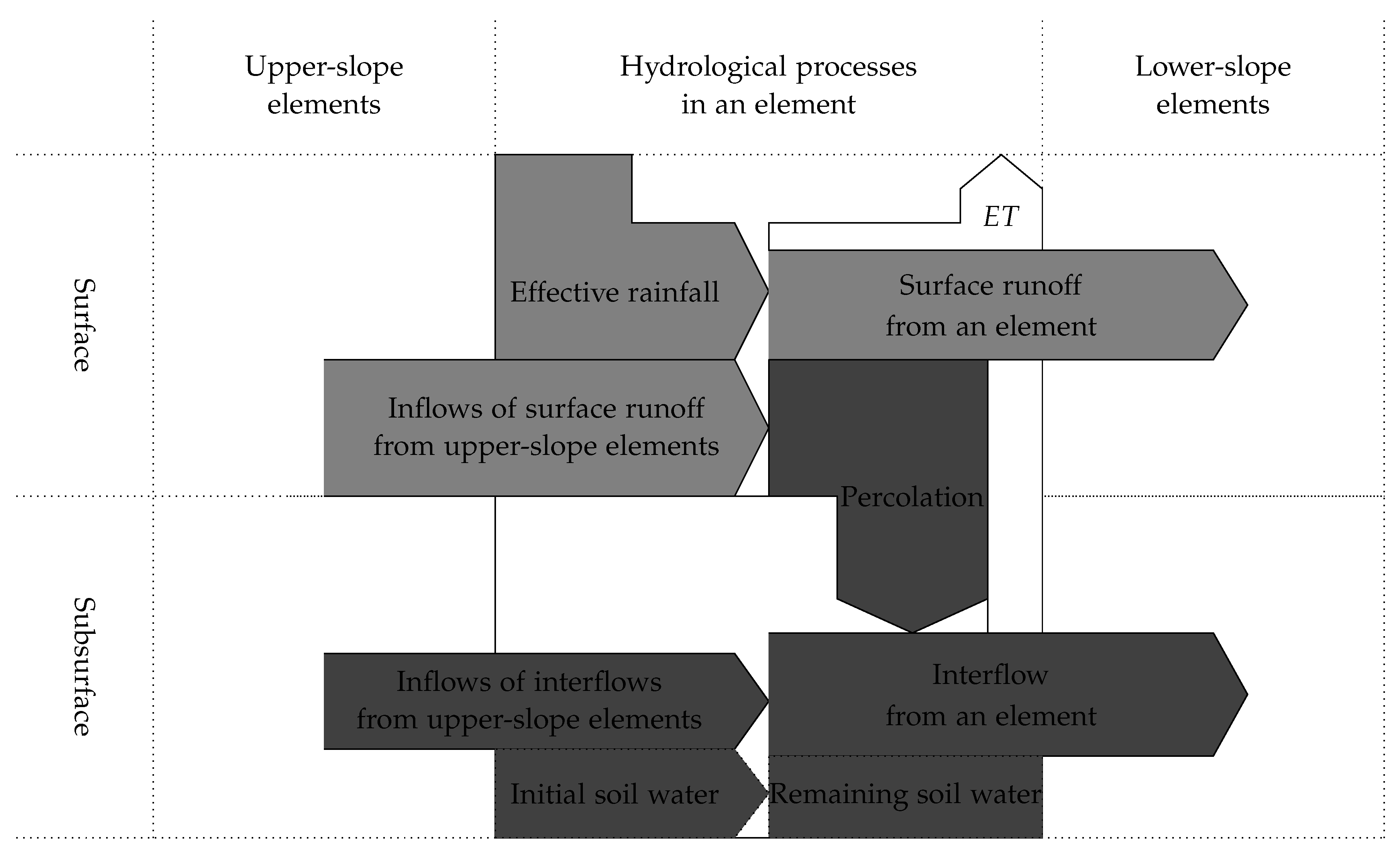
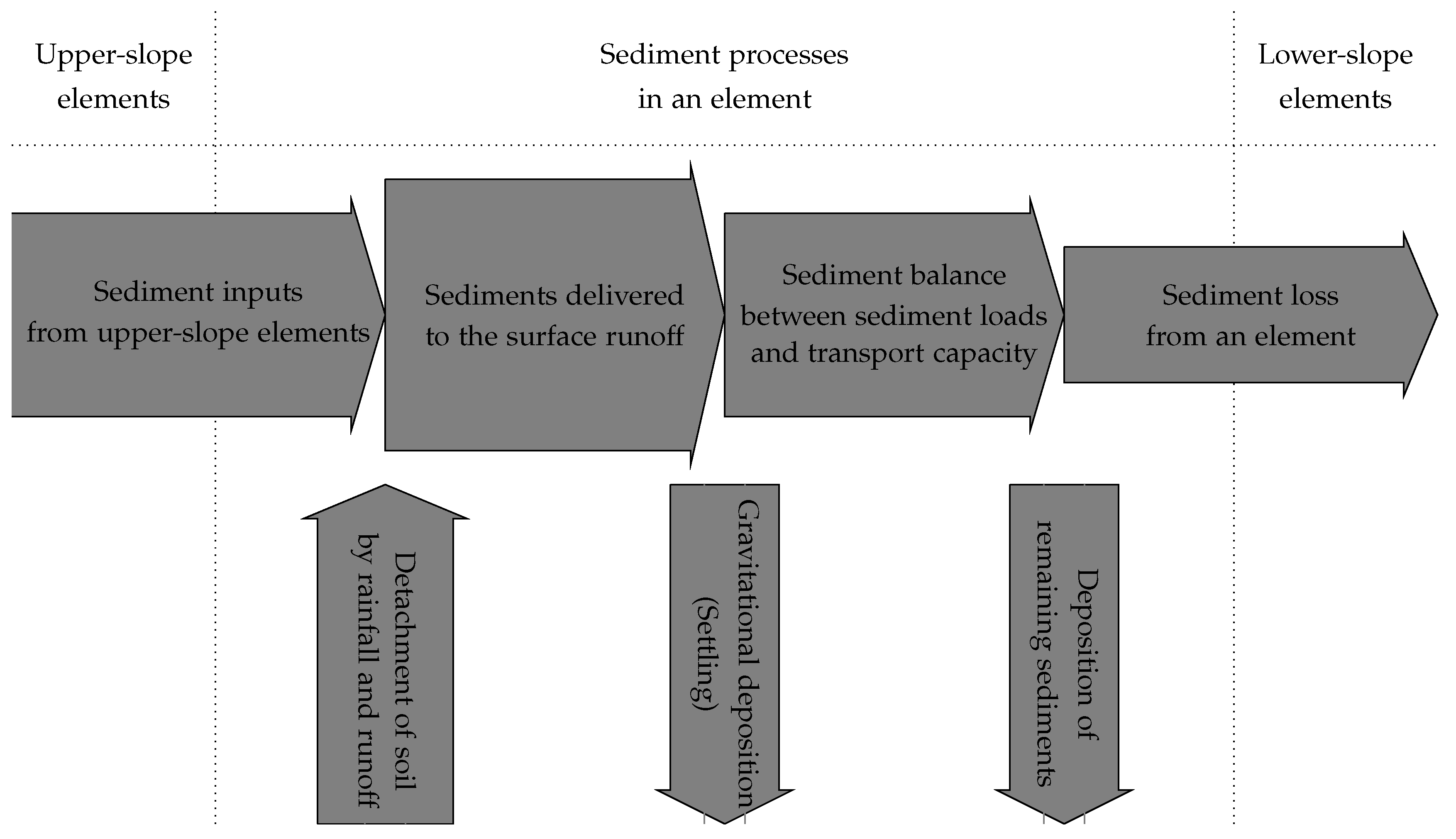
The DMMF model can estimate the amount of surface and subsurface water input from the upslope area and output to the downslope area after hydrological processes for each element (e.g., each grid cell in a raster map). The model also estimates the sediment budget of each element by calculating the amount of sediments flowing into and out of the element. The hydrological processes of the model are determined by rainfall, evapotranspiration, surface/subsurface water inflows, and initial soil water content (Figure 2). After calculating the water budget for the element, the model calculates sediment budgets, considering the amount of sediment input from the upslope areas, rainfall intensity, topography, soil characteristics, surface configurations, and vegetation structures (Figure 3). The detailed input parameters are presented in Table 1 and detailed structure and equations are described in the Appendix A.
In contrast with the SWAT model, which has been frequently applied to this catchment, the DMMF model can estimate the erosion and deposition of an element, considering the interconnectivity with adjacent elements. Therefore, the model can be used to estimate the impact of the spatial reconfiguration of erosion hot spots into forest on sediment yields more explicitly for each element and the entire catchment.

2.3. Model Parameterization

As shown in Table 1, the DMMF model requires the topography, climate, soil, and LULC datasets to project surface runoff and sediment redistribution patterns of the catchment.
Topography data (i.e., the slope angle (S) and grid size of a raster map ( r e s )) were derived from the digital elevation model (DEM) with 30 m resolution. The parameter r e s is used to calculate the width (w) and length (l) of an element that are equivalent to r e s and r e s / cos ( S ) , respectively [15].
Climate data were obtained from two sources. The daily rainfall (R) and mean rainfall intensity of a day ( R I ) were obtained from weather stations installed in the catchment, and the evapotranspiration ( E T ) was obtained from remote sensing data provided by the Moderate Resolution Imaging Spectroradiometer (MODIS) [43]. We estimated R and R I from each weather station and spatially interpolated them using inverse distance weighted (IDW) method, which showed the optimal result on this catchment among four methods such as inverse distance weighted, spline, nearest neighbor, and kriging, according to Shope et al. [30]. For the E T , we resampled the 8-day average MODIS/Terra Evapotranspiration data to fit to the DEM of this catchment.
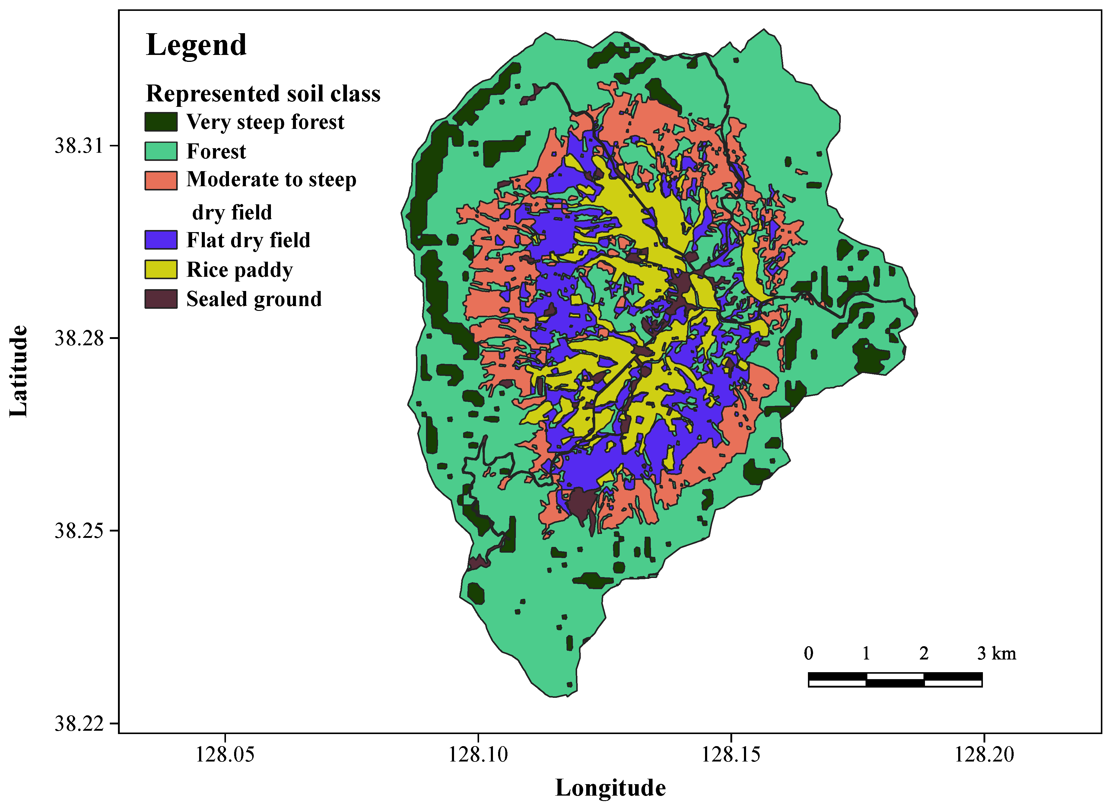
The soil data set covers the texture, depth, hydraulic properties, and detachabilities. The soil texture (i.e., the proportion of clay ( P c ), silt ( P z ), and sand ( P s ) in the surface soil), soil depth ( S D ), and soil hydraulic properties (i.e., saturated soil water content ( θ s a t ), soil water content at field capacity ( θ f c ), and saturated lateral hydraulic conductivity (K) of the entire soil profile) were derived from a 2009 catchment-wide field survey from the TERRECO project (see Table 2 and Figure 4) [30].
Reference values for soil detachability from Morgan and Duzant [40] were used as the initial values of soil detachability by rainfall (i.e., for clay ( D K c ), silt ( D K z ), and sand ( D K s )) and by runoff (i.e., for clay ( D R c ), silt ( D R z ), and sand ( D R s )). We assumed that the initial soil water content of the entire soil profile ( θ i n i t ) is equal to the soil water content at field capacity ( θ f c ) by starting the simulation at three days after the first heavy rainfall of the year, because the excess soil water was usually drained away two or three days after the soil was fully saturated by rainfall.
The LULC types characterize the physical structures of surface and vegetation, which regulate the quantity of surface runoff and runoff velocity. Surface structures incorporate a portion of the impervious cover area ( I M P ), such as plastic mulching and paved facilities, flow depth of surface runoff ( d a ), and Manning’s roughness coefficient of the soil surface (n). Vegetation structures contain the permanent interception of rainfall ( P I ), pervious ground cover ( G C ), canopy cover ( C C ), average vegetation height ( P H ), average diameter of individual plant elements at the surface (D), and number of individual plant elements per unit area ( N V ). LULC parameters were derived based on the LULC map of the Haean catchment in the year 2010 from Seo et al. [35] (see Figure 5).
We classified the original LULCs into 14 categories (i.e., forest, rice paddy, semi-natural, bare soil, ginseng, potato, bean, radish, cabbage, other dry crops, shrub, orchard, urban, and water bodies). Forest, rice paddy, semi-natural, bare soil, ginseng, potato, bean radish, and cabbage are major LULCs that covered more than 1% of the catchment area. Minor LULCs were aggregated into groups of other dry crops, shrub, orchard, urban, and water bodies according to their physical characteristics. We used field measurement data of C C , P H , N V , I M P , d a , and n for major dry crops such as bean, cabbage, potato, and radish, whose data were obtained from the field campaign of the TERRECO project, which was also used in Arnhold et al. [17]. The daily forest C C was estimated using the average values of 8-day normalized difference vegetation index (NDVI) for forest in the catchment from MODIS [45,46]. The average NDVI values were converted to canopy cover ( C C ), using the equation suggested by Gutman and Ignatov [47]. LULC parameters for rice and ginseng, and the average diameter of individual plant elements (D) for major dry crops were obtained from agricultural technology portal provided by Rural Development Administration of South Korea (RDA) [48]. The average LULC parameters of major dry crops were used for the LULC parameters of other dry crops, while the guide values from Morgan and Duzant [40] were adopted for other LULC parameters. Detailed initial parameter settings are presented in Table 3.

2.4. Model Calibration and Validation

The DMMF model was calibrated and validated for stream discharge and suspended sediment to test its performance in the Haean catchment. The testing was performed utilizing data from the year 2010 when the LULC map, as well as the field-measured stream discharge and suspended sediment data, were well established [30,35]. We confined the testing period from the 67th day of the year (DOY), which is three days after first heavy rainfall of the year, to reduce the uncertainty of initial soil water content by equating it with the soil water content at field capacity. We equalized the two parameters based on the field measurement guidelines for soil water content at field capacity, which recommend soil sampling two or three days after rainfall that is heavy enough to saturate the soil. The three sub-catchments of S1, S2, and S3 (see Figure 1) were selected for model calibration and validation. The data from the S1 and S2 were utilized for two-step calibration, and those from the S3 were used for model validation. Two-step calibration was performed on the forest-related parameters utilizing the data from the S1 site, and the other parameters were calibrated utilizing the data from S2. This calibration method enables us to prevent the significance of forest-related parameters of dominant LULC type in the entire catchment, from overtaking the importance of other parameters, resulting in those parameters being ignored. The DMMF model can estimate the outputs of the surface and subsurface runoff, and the sediment from the elements. However, the measured data are stream discharge and suspended sediments at the outlet of each sub-catchment. Because the model does not consider in-stream processes and the impact of groundwater on the base flow of the stream, it is not appropriate to directly compare the result from the model with the measured data. To match different comparative objects, we compared the total daily discharge of each site to total daily surface runoff and subsurface interflow flowing into the stream from the model, while adding a constant corresponding to base flow from groundwater. To match the sediment yield from the terrestrial part with the suspended sediments measured at the outlet of each sub-catchment, we should consider the in-stream sediment processes and impact of erosion control facilities. Reflecting sediment deposition on the stream bed load, we assumed that only a part of the terrestrial sediment yield entering the stream was sampled at each measuring point for each sub-catchment. Therefore, we compared the suspended sediments measured from the outlet of each measuring point to the sediment flowing into the stream from the model, multiplied by a constant, reflecting the in-stream sediment process. Our assumptions can be described as below,
Q m = Q s + I F s + α ,
S L m = β × S L s .
Here, Q m represents the measured daily total discharge, and Q s , I F s , and α represent the daily surface runoff, daily subsurface interflow simulated from the DMMF model, and a constant reflecting the base flow from groundwater (unit: m 3 / s ). S L m represents the total daily suspended sediments measured at the outlet of each sub-catchment, and S L s and β represent the terrestrial sediment yield entering the stream from the model simulation and constant representing the in-stream sediment deposition rate, respectively.

2.4.1. Sensitivity Analysis

To select important parameters to be calibrated among unmeasured or highly uncertain parameters, we performed site-specific sensitivity analyses, using the Sobol’ method [50,51,52]. The Sobol’ method is a variance based sensitivity analysis that is widely used in environmental and hydrological modeling, such as SWAT and TOPMODEL [53,54]. This method can estimate the total effect of each parameter on the model output, considering the combined effects among parameters. Therefore, the Sobol’ method is more suitable for analyzing the sensitivity of non-linear and non-additive models containing many parameters, as opposed to the local or one-at-a-time (OAT) methods [53,55]. The relative sensitivity of parameters is expressed as the Sobol’ total index (SI)—the ratio of the amount of total variance caused by a parameter to the amount of variance induced from all parameters (i.e., the unconditional variance of the model) [52]. If we have p-dimensional parameter set, the first-order sensitivity of the i-th parameter can be described as,
S i = V X i ( E X i ( Y | X i ) ) V ( Y ) ,
where V X i ( E X i ( Y | X i ) ) is the variance of the model solely by i-th parameter ( X i ). Then the total sensitivity of the i-th parameter ( S I i ) can be calculated as below,
S I i = 1 V X i ( E X i ( Y | X i ) ) V ( Y ) ,
where V X i ( E X i ( Y | X i ) ) V ( Y ) indicates that the sum of first-order sensitivities of all parameters except i-th parameter. Parameters with large SI indicate a relatively high impact on the model output, while those with small SI indicate a relatively low impact on the model output.
Because the soil hydraulic parameters (i.e., θ s a t , θ f c , and K), soil detachabilities (i.e., D K c , D K z , D K s , D R c , D R z , and D R s ) and LULC parameters (i.e., P I , I M P , G C , C C , P H , D, N V , d, and n) were not measured or had high uncertainties, their importance was tested on model outputs. Before performing sensitivity analysis, we set the range of the parameters to be tested. The ranges of soil hydraulic parameters (i.e., θ s a t , θ f c , and K) were set based on the range of estimated values for each represented soil class (see Table 2). The upper bound of θ f c was set as the minimum θ s a t , and the upper bound of K was set to 18 times of the maximum K to reflect high uncertainty of the parameter [56]. The ranges of the un-measured LULC parameters were set based on the initial parameter settings for each LULC type (see Table 3). We adjusted the parameters using a range of ± 100 % for the initial parameter settings for each LULC type. If the upper or lower limits of the proportional parameters is out of the range between zero to one, we set the lower limits to zero and the upper limits to one. In this study, SIs for the input parameters were estimated using the “sobolmartinez” function of the “sensitivity” package [57] on R version 3.5.1 [58], a well-established open-source program for statistical computing, providing many analysis packages. We used the default bootstrapping option of the function, employing a sample size of 10 3 .

2.4.2. Calibration

To find the optimal combination of the parameter set, which allows model outputs to explain the measured stream discharge and suspended sediments from each site, we performed two-step calibration. For each step, we adjusted the important parameters with SI greater than 0.05 (i.e., contributing 5% of the total variance), and we adjusted the constants for the in-stream processes ( α and β ) additionally for sub-catchment S2, where data were measured in the stream outlet. We searched for the optimal combination of the parameter set, using the differential evolution (DE) optimization method [59,60]. The DE algorithm is a heuristic optimization method with an evolution strategy for finding the global optimum value. Requiring few prerequisites for its execution, the algorithm is applicable to non-differential, nonlinear, and multimodal models. As a result, the DE algorithm has been applied to a variety of fields including hydrological model calibration [15,59,60,61,62,63]. We applied the DE algorithm for model calibration using the “DEoptim” package [61,64] on R version 3.5.1 [58]. We used the Nash-Sutcliffe efficiency coefficient (NSE) [65] between model outputs and field-measured data as an objective function for the DE algorithm. To treat NSE values from stream discharge and suspended sediments fairly, we evaluated the NSE values for each measurement and used the average NSE value as the final objective function:
F o b j = 1 NSE ( Q m ) + NSE ( S L m ) 2 ,
where F o b j is the objective function to evaluate the model performance. We ran the function for 10 3 iterations, and ran for three different initial states to try to find the global minimum as an optimum value.

2.4.3. Validation

Using adjusted parameters from calibration steps, model performance was tested for the S3 site, which is located near the catchment outlet. Considering site-specific base flow from groundwater and in-stream sediment processes for the S3 site, we adjusted the constants for the in-stream processes ( α and β ). We utilized the NSE, the percent bias (PBIAS), and the coefficient of determination ( R 2 ) as statistical criteria for model performance evaluation [66,67]. The function “gof” from the “hydroGOF” package [68] in R version 3.5.1 [58] was used to evaluate statistical criteria.

2.5. Identifying Annual Sediment Redistribution Patterns and Assessing Soil Erosion Risk

Projecting validated parameters on the DMMF model, we simulated and calculated the annual sediment redistribution patterns of the catchment. Based on the simulated result, we assessed the net soil erosion rate ( S L n e t : t / h a / year ) for each element of the catchment. S L n e t is the net soil erosion for each element, which is the amount of sediment input to each element from upslope elements ( S L i n ) subtracted from the amount of sediment output from the element ( S L o u t ). Soil erosion risk was assessed by using S L n e t of each element. We classified S L n e t into five categories, namely tolerable, low, moderate, high, and severe, as shown in Table 4 according to the soil erosion risk categories defined by OECD [69,70] which is one of the internationally used criteria.
Based on the net soil erosion rate of the entire catchment, we assessed the soil erosion characteristics for each LULC class. For the assessment, we calculated the mean S L n e t for each LULC class.

2.6. Evaluation of the Impact of Spatial Reconfiguration of Erosion Hot Spots into Forest

We assessed the impact of the spatial reconfiguration of erosion hot spots into forest, based on the annual sediment redistribution patterns of the catchment. Erosion hot spots represent elements in which much annual net soil erosion ( S L n e t ) occurs. To compare the impact of spatial reconfiguration, we calculated the annual sediment yields being generated from the terrestrial area and entering to the water bodies of the entire catchment ( S Y b a s e ) as a base line condition. S Y b a s e is the total amount of sediment yields entering the water bodies of the entire catchment, which is equal to the total amount of S L i n flowing into water bodies. To increase the robustness of our analysis, we only used the values between the 2.5th percentile and the 97.5th percentile for all the elements in the catchment to exclude the impact of extreme values that can occur from model outputs. The lower extreme values were set to the value of the 2.5th percentile and the upper extreme values were set to the value of the 97.5th percentile. The impact of the spatial reconfiguration of erosion hot spots into forest was evaluated by calculating the total annual sediment yields entering the stream ( S Y t o t ), using the DMMF model as bare soil and croplands (i.e., bean, cabbage, ginseng, orchard, potato, radish and rice field) being sequentially changed into the forest. We selected forest, the original LULC type before anthropogenic land cover changes, as the alternative LULC to mitigate erosion-prone areas. Similar to the methods Chaplin-Kramer et al. [23] and Chaplin-Kramer et al. [24] which compute ecosystem services by marginally changing forest into agricultural areas, we computed S Y t o t by gradually converting 1% of the bare soil and croplands in the catchment into forest until all bare soil and croplands elements are converted into forest. Based on this result, we presented the total sediment yields ( S Y t o t ), reduction rate of the sediment yields entering the stream compared to base line condition ( S Y b a s e ), and sediment yield reduction efficiency per conversion area ( t / m 2 ).

3. Results

3.1. Model Performance

According to the calibration and validation results, the DMMF model showed competitive performance, predicting stream discharge, but showed poorer performance in evaluating the amount of suspended sediments at the outlet of each sub-catchment. We performed two-step calibration by comparing the model outputs to the measured data collected from sub-catchment S1 and S2. The LULC and soil types of sub-catchment S1 are classified as forest and forest soil, according to Table 2 and Table 3. The calculated Sobol’ index for important parameters, both for stream discharge ( S I Q ) and suspended sediments to the stream ( S I S L ) , are presented in Table 5.
According to the Sobol’ index, the amount of stream discharge was highly influenced by the permanent interception of rainfall ( P I ) and lateral soil hydraulic conductivity (K), which regulate the amount of rainfall and flow rate of subsurface interflow of the sub-catchment, respectively. Vegetation and surface cover structures ( G C , P I , and d a ), detachability of clay particles ( D R c ), soil water content at field capacity ( θ f c ), and lateral soil hydraulic conductivity (K) exhibited a relatively large impact on suspended sediments generated from the sub-catchment. This result indicates that the suspended sediments generated from the sub-catchment are determined by the amount of surface runoff and the erosivity of surface, because P I , K, and θ f c determine the amount of surface runoff by regulating the amount of rainfall and partitioning the rate of surface and subsurface water. Parameters G C , d a , and D R c determine the erosivity by surface runoff.
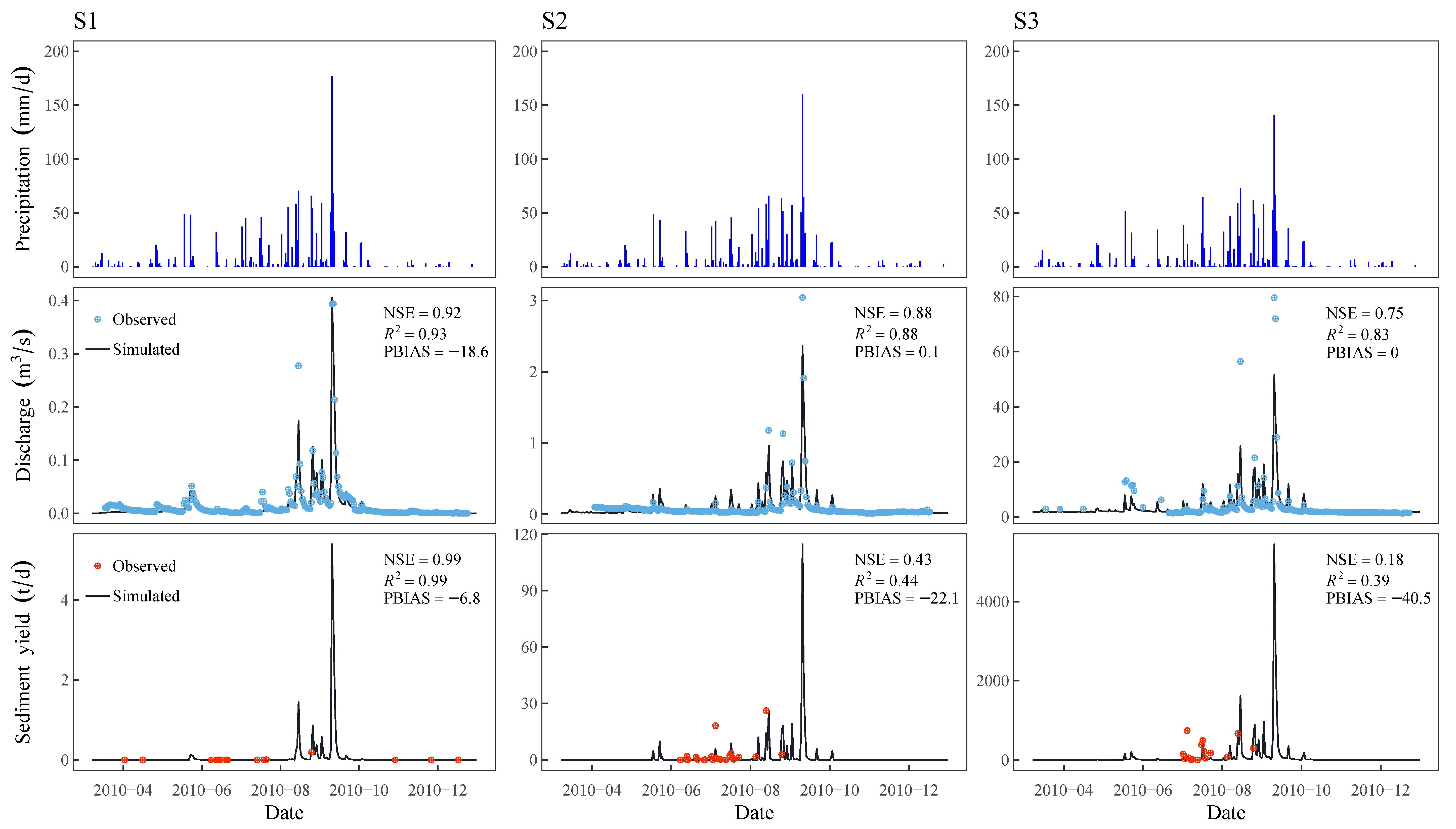
We determined an optimized parameter set by adjusting selected important parameters from sensitivity analysis using the DE algorithm (see Table 5). With the optimized parameter set, the stream discharge and suspended sediment from the model outputs were compared with those from field measurements (see Figure 6).
After calibrating the forest-related parameters, we calibrated the other parameters, based on the measurement data collected from sub-catchment S2. We calculated the relative importance of parameters for both the stream discharge ( S I Q ) and suspended sediments to the stream ( S I S L ) , using the Sobol’ index, and presented them in Table 6.
According to sensitivity analysis, model outputs were highly sensitive to soil hydraulic characteristics of moderate to steep dry field soil and land cover structures of the semi-natural field. In details, the stream discharge of the sub-catchment was highly sensitive to the permanent interception of rainfall ( P I ) of the semi-natural, rice paddy, and other dry crops; the lateral hydraulic conductivity (K) of the moderate to steep dry field and flat dry field soils; and the soil water content at field capacity ( θ f c ) of the moderate to steep dry field. This result indicates that stream discharge is highly influenced by the amount of rainfall reaching the ground ( P I s) and the flow rate of subsurface interflow (Ks and θ f c ) of this region. The sediment yield to the stream is sensitive to the soil detachability by runoff ( D R c and D R z ) of the moderate to steep dry field soil, soil water content at field capacity ( θ f c ) of the moderate to steep dry field soil, flow depth ( d a ) of the semi-natural field and bean field, and ground cover ratio ( G C ) of the semi-natural field. This result emphasizes the role of the moderate to steep dry field soil, which is the second largest soil type, following forest soil, and demonstrates the crucial role of the semi-natural field on determining suspended sediment output from the model.
The performance statistics for the calibration and its time series plots of observed versus simulated stream discharge and suspended sediment were presented in Figure 6. For the calibration steps, the NSE values for stream discharge were 0.92 and 0.88 for sub-catchment S1 and S2, respectively. The R 2 values for stream discharge were 0.93 and 0.88, respectively, and the PBIAS values for stream discharge were −18.6 and 0.1, respectively. The NSE values for suspended sediment were 0.99 and 0.43 for sub-catchments S1 and S2, respectively. The R 2 values for suspended sediment were 0.99 and 0.44, and the PBIAS values for suspended sediment were −6.8 and −22.1 for the sub-catchments, respectively. The site-specific constants reflecting the baseflow from groundwater ( α ) and in-stream sediment deposition rate ( β ) for sub-catchment S2 are 1.75 × 10⁻²m3/s and 4.57 × 10⁻². In validation steps, the NSE values for stream discharge and suspended sediment were 0.75 and 0.18, respectively, with the site-specific α and β being 1.711 m 3 / s and 6.76 × 10⁻², respectively. The R 2 for discharge and sediment were 0.83 and 0.39, respectively, and the PBIAS for discharge and sediment were 0 and −40.5, respectively. According to the model performance evaluation criteria suggested by Moriasi et al. [67], the DMMF model showed good performance for discharge in both calibration and validation steps. Though there is no clear model performance evaluation criteria suggested for daily time scale sediment result for watershed model due to limited reported data [67], When we apply the performance evaluation criteria for monthly time scale sediment result for watershed scale model, the model might be considered to have a slightly poor performance for sediment during the calibration and validation steps, as the NSE and R 2 values were less than 0.45 and 0.40, respectively.

3.2. Sediment Redistribution Pattern of the Catchment

Simulating the model with optimized parameters, we calculated the annual net soil erosion rate ( S L n e t ) for each element and classified them into five classes–tolerate, low, moderate, high, and severe—as in Figure 7.
According to Figure 7, elements with severe soil erosion (>33 t / h a / year ) were concentrated on the dry crop field with moderate to steep slope conditions on the interface with the forest. The estimate of the mean annual net soil erosion rate by each LULC type (Table 7) shows that bare soil and dry crop field suffered from severe soil erosion. On the other hand, forest, rice paddy, orchard, and urban areas showed good sediment capturing capabilities.

3.3. Impacts of Conversion of Erosion Hot Spots into Forest on Total Sediment Yield Entering the Stream

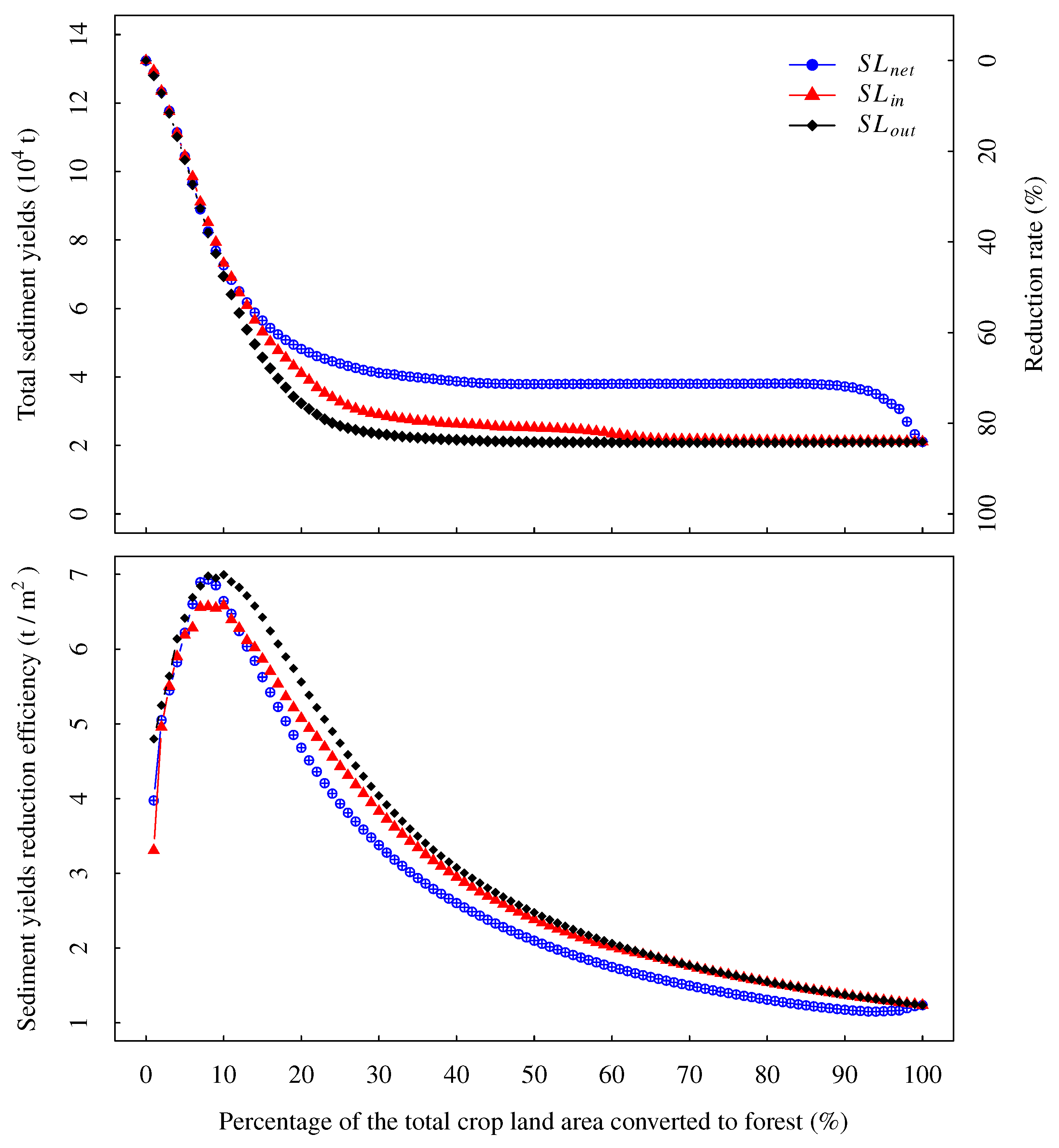
The LULC conversion of erosion hot spots into forest showed a dramatic impact in the reduction of sediment yields entering the stream, as shown in Figure 8.
When each bare soil and crop field element in the catchment was converted into the forest sequentially from the area with the highest soil erosion rate to the area with the lowest soil erosion rate, the amount of total annual sediment yield of the catchment to the stream sharply decreased having a shape similar to an inverted sigmoid function. Changing the 3% of erosion hot spots that have suffered the most from severe soil erosion caused a reduction in sediment yield entering the stream of ca. 10% from the baseline condition ( S Y b a s e ), and a change in 10% of most severe hot spots is expected to reduce sediment yields by ca. 50%. Among the elements S L n e t , S L i n , and S L o u t , the altered areas revealed that outputs from the element ( S L o u t ) proved to be the most effective in reducing the total sediment yield into the stream. A simulation of the sediment yields entering the stream showed that the reducing rate in sediment yield for S L n e t was less effective than those for S L o u t and S L i n . Due to total annual sediment yields sigmoidally decreases as bare soil and crop fields begin changed into forest, sediment yield reduction efficiency per unit conversion area increased until ca. 10% of total crop land area converted to forest and then gradually decreased. A simulation of the sediment yield reduction efficiency showed that the element ( S L o u t ) was most efficient for all conversion intervals.

4. Discussion

Our findings emphasize the importance of landscape configuration on regulating ecosystem services by showing the effectiveness of spatial reconfiguration of soil erosion hot spots into forest on reducing the amount of sediment yield entering the stream. We simulated the annual sediment redistribution pattern in the Haean catchment, utilizing the daily based Morgan–Morgan–Finney (DMMF) soil erosion model. According to the result, the soil erosion rate varied greatly depending on the topography and LULC type, and the area located on the steep hill-slope, which is adjacent to the forest severely suffered from soil erosion. When reconfiguring the landscape patterns of croplands by sequentially altering erosion hot spots from the most severe to the least severe areas into forest, we found dramatic effects in the reduction of sediment yields entering the stream in this catchment. The reduction rate may reach ca. 50% when the 10% most severe erosion hot spots were altered, and we can expect a reduction rate of over 80% when the ca. 20% most severe erosion hot spots are altered. In the following, we first discuss model performance and limitation, and then potential management implications.

4.1. Model Performance

The assessment of soil erosion risk and measurement of the effectiveness of the spatial reconfiguration of erosion hot spots in reducing sediment yields entering the stream were based on the calibrated and validated simulations of the DMMF soil erosion model. According to the model performance criteria from Moriasi et al. [67], the DMMF model showed satisfactory performance for predicting stream discharge during the calibration and validation processes, with mean NSE values of 0.90 and 0.75, mean R 2 of 0.91 and 0.83, and maximum PBIAS of −18.6 and 0 during calibration and validation steps, respectively. The model showed comparatively poor performance for predicting suspended sediment at the outlet of each sub-catchment, except the small forested site (S1) where the stream does not exist. The mean NSE values were 0.66 and 0.18, mean R 2 were 0.67 and 0.39, and maximum PBIAS were −22.1 and −40.5, respectively. When we compared the model performance statistics of the DMMF model to those from previous studies using soil and water analysis tool (SWAT), the model showed competitive performance in predicting stream discharge but poorer performance in terms of predicting suspended sediments in the stream [3,19]. Maharjan et al. [3] reported that mean NSE values for stream discharge were 0.82 during calibration and 0.45 during validation. In addition, they showed that mean NSE values for suspended sediment were 0.78 and 0.60 during calibration and validation, respectively. Jang et al. [19] also reported mean NSE values for stream discharge of 0.78 and 0.66 during calibration and validation, respectively. They reported mean R 2 for suspended sediment were 0.80 and 0.76 during calibration and validation, respectively. In terms of soil erosion rate for each crop field, the DMMF model estimated that the average annual soil loss of major dry crops ranged between 79.3 t / h a / year and 763.8 t / h a / year for bean, radish, potato, and cabbage, and the average annual soil loss from whole dry crop fields was 379.7 t / h a / year . Arnhold et al. [17] reported that 30–54 t / h a / year of soil loss occurred in the dry crop fields, including bean, radish, potato, and cabbage, from the plot-level field measurement. Furthermore, Maharjan et al. [3] estimated that 35.5–53.0 t / h a / year of soil loss occurred in the dry crop fields from the SWAT model. When we compared the results from the DMMF model with those from other studies, the amount of soil loss from this study is far greater. The reasons that the DMMF model showed poor performance for predicting suspended sediment in the stream can be analyzed from two perspectives. The first reason involves the discrepancy of data types between the DMMF model and observed data. The observed data were stream discharge and suspended sediment at the outlet of each sub-catchment. On the other hand, the DMMF model can estimate the total sediment yields entering the stream that belongs to each sub-catchment. The DMMF model is efficient for estimating sheet and rill erosion, but it has limitations in estimating in-stream sediment processes such as stream bed deposition, channel erosion, and sediment transport in the stream. Considering the limitations of the model, we use site-specific coefficients, which assume that suspended sediments measured at the outlet are proportional to the sediment yields inflowing into the stream. However, incorporating the quantity and the velocity of stream water discharge, sediment flux, and physical characteristics of channel structures such as gradient, width, depth, and length, into the in-stream sediment process, is complicated [71,72]. The reasons above may lead to a high sediment deposition rate in the stream (i.e., low measured sediment ratio ( β )), which in turn, causes a high soil erosion rate in the terrestrial area. Because the study sites are affected by monsoon climate, such that its rainfall pattern is not uniform but rather with a lot of extremes, a large amount of sediment is deposited during low rainfall events, and the deposited sediments are washed out by a huge amount of fast stream discharge accompanying heavy rainfall. Temporal lags between the rainfall event and stream discharge are negligible for the Haean catchment, but for suspended sediments, the lags are significant and highly depend on the stream length because of the difference in travel velocities between water and soil particles [73,74,75,76]. Therefore, the model performance for predicting stream discharge may be better than that for predicting suspended sediments. The stream widens and deepens as it descends to the lower area, according to Lee [2], and the length of the stream also increases as the size of sub-catchment grows. The uncertainty caused by in-stream processes increases as the size of the sub-catchment grows, which reduces the model performance in predicting suspended sediments in this study. SWAT and USLE-based models are usually calibrated and validated at the fixed spatial area with a different temporal period. Therefore, in-stream sediment processes can be included in the parameters, which may lead to better model performance. However, the DMMF model is a spatially distributed semi-processed model and used the same temporal period with a different spatial area for calibration and validation in this research, so that the in-stream processes cannot be included in the model.
Secondly, many sediment reduction facilities, such as dams for freshwater, debris barrier and culvert systems around crop fields, and road infrastructures, which can affect sediment transport processes, have been installed in the Haean catchment [30,36]. The dam and debris barriers create reservoirs that impede the stream flow and filter out sediments in the facilities. This disrupts the correct evaluation of the model performance for this catchment. Shope et al. [30] showed complex stream networks, including the culvert systems around crop fields and the road infrastructure. The culvert systems extend the travel time of suspended sediments and reduce the runoff and transport velocities of sediments by altering the flow direction abruptly. Increased travel time and decreased transport velocity tend to increase the deposition rate of sediments compared to the condition without the culvert system. The deposited sediments in the culvert flow into the stream by runoff, with sufficient power to wash out. The culvert system is also responsible for the temporal lag between the rainfall event and the presence of suspended sediments in the catchment. Sediment reduction facilities trap a huge amount of sediments, which make the measured sediment ratio ( β ) in this study have very low values. Because of the small β , the stream bed deposition rate became too large, and consequently, the overall erosion rate from terrestrial area increased. To cope with this problem, the in-stream processes will need to be considered more precisely through model improvements.

4.2. Assessment of Soil Erosion Risk and the Effectiveness of Spatial Reconfiguration of Erosion Hot Spots on Reducing Sediment Yield Entering the Stream

We estimated the annual net soil erosion rate of the entire catchment and assessed the soil erosion risk class according to the OECD criteria. According to this study, soil erosion is concentrated on the hill-slope of the catchment, and the problem is more significant for the bare soil and dry crop fields, such as bean, radish, and potato, in this area. In addition, forest in the valley showed a considerable amount of soil loss, also suffering from erosion due to the concentrated surface runoff and steep slope. Compared with other studies, the soil erosion risk pattern and the average annual soil loss from the DMMF model is qualitatively consistent with the soil erosion risk map from Lee et al. [77], with average climate conditions for the 2010s using the USLE-based SATEEC [78] model. According to this study, urban area, orchard, and rice field showed better performance for sediment capturing capabilities than forest. However, the urban area and rice field are located in the lower and flatter area than forest, so that the sediment inputs from the upslope area tend to be deposited in this area. Furthermore, because the urban area is usually paved with impervious covers, such as concrete and asphalt, and the rice field is filled with water, which acts as a pervious cover that prevents surface erosion, these areas have little soil loss but receive huge input from the upslope area. Though the forest is in a region where the slope is very steep, the average amount of soil loss is smaller compared with other land types, and it also shows excellent sediment capturing capability, in general. Like the other studies, we can conclude that the main cause of severe erosion in the catchment is cropland extension after deforestation at the hill-slope area of the catchment [2,3,11,17,19,77]. We also assessed the effect of spatial reconfiguration of LULCs on reducing sediment yields entering the stream. In this study, the spatial reconfiguration of erosion hot spots into forest showed excellent reduction efficiency in sediment yields entering the stream. We identified that the sediment yields entering the stream were reduced sharply, as crop lands were sequentially changed into forest from the area with the most severe soil loss to the area with the least soil loss. An sigmoidal sediment reduction rate from altering LULCs to forest indicates that forest is not only effective in preventing surface erosion but also effective in capturing sediment input from the upslope area. In addition, the result suggested that altering LULCs based on the amount of sediment output from the element is the most effective way of reducing sediment yields entering the stream. This result is consistent with previous studies that emphasize the effectiveness of vegetative filter strips located at sediment sources such as crop fields [3,5,19,27,28,29]. The result can also be generalized to consider the effect of riparian vegetation buffer strip on reducing sediment yields entering the stream, located at the interface between crop fields or natural sediment sources and the stream channel [4,79,80]. This study also demonstrated that the sediment yield reduction efficiency initially increased as the first few bare soil area and crop lands with the most severe soil loss were converted into forest. The sediment yield reduction efficiency were maximized when ca. 10% of the area converted, and then the efficiency decreased gradually. These patterns can be explained by two aspects of the forest’s sediment yield reduction capability; protecting surface from soil erosion, and capturing sediment inputs. The areas with the most severe soil loss are located at the steep hillslope where surface runoff is concentrated. These areas have a large transport capacity of the runoff, beyond the sediment capturing capability of forest because transport capacity is greater than the available sediment for transport [15]. In these areas, conversion of crop lands into forest can reduce soil loss from the surface but cannot capture sediment inputs from upslope which is larger than surface soil loss. As slope becomes milder and the amount of surface runoff decreases due to gradual conversion of crop lands into forest, transport capacity gradually decreases. Decreased transport capacity caused by decreased slope gradient and surface runoff lets forest capture more sediments, maintaining the surface protecting capability from soil loss. Therefore, the sediment yield reduction capabilities of forest become small and the sediment yield reduction efficiency by changing crop lands into forest decreases gradually. According to these results, one can reduce sediment yields entering stream efficiently by identifying an optimal percentage of crop land conversion into forest which brings out the best efficiency of sediment yield reduction per unit conversion area.

5. Conclusions

In this study, we identified the soil erosion risk of Haean catchment spatially explicitly by projecting sediment redistribution patterns using the DMMF model. In addition, we measured the sediment yield reduction efficiency entering the stream by sequentially altering erosion hot spots into forest from that which has the highest soil loss to that which has the lowest soil loss. The DMMF model showed competitive performance estimating stream discharge but exhibited lower performance estimating suspended sediments at each sub-catchment outlet. When we applied the DMMF model to the Haean catchment, the bare soil surface and dry crop fields located on the steep hill-slope of the catchment suffered mostly from severe soil erosion. On the other hand, forest, rice paddy, orchard, and urban areas suffer less from soil erosion. By changing the erosion hot spots from cropland to forest, the overall amount of sediments exporting to the stream of the catchment was effectively reduced. The sediment yield reduction efficiency was maximized when ca. 10% of crop lands were converted to forest. This study implies that one can achieve the goal of reducing sediment yields entering the stream by identifying the location of erosion hot spots and managing the area intensively. Although previous studies showed good mitigation effects of BMPs that require compliance of stakeholders, this may not be easy and takes much time for stakeholders to follow the BMPs, because the degree of acceptance of the policy depends on the situation and tendency of each stakeholder [19]. On the other hand, the spatial reconfiguration approach proposed in this study can reduce the number of stakeholders relevant to soil erosion mitigation measures. However, this approach reduces crop yields because crop lands are converted to non-crop lands to reduce sediment yields from the catchment. In addition, the sediment yield reduction efficiency decreases after a certain point of spatial reconfiguration. Therefore, the two approaches—BMP measures such as cultivating cover crops, mulching surface with straw, and managing field margin naturally, and conversion of crop lands with the more severe soil loss—are complementary measures to reduce sediment yields into the stream.

Author Contributions

Conceptualization, K.C. and B.R.; Data curation, K.C. and G.R.M.; Formal analysis, K.C.; Investigation, K.C.; Methodology, K.C.; Resources, G.R.M.; Software, K.C.; Supervision, B.R.; Validation, K.C.; Visualization, K.C.; Writing original draft, K.C.; Writing review & editing, G.R.M. and B.R.

Funding

This study is part of the International Research Training Group “Complex Terrain and Ecological Heterogeneity” (TERRECO) funded by the German Research Foundation (DFG) with the grant number [GRK 1565/1]. This study was also supported by the National Research Foundation of Korea (NRF) with the grant number [NRF-2017R1A2B4010460].

Acknowledgments

This paper is dedicated to the memory of our wonderful colleague, Sebastian Arnhold, who passed away last year. This publication was funded by the German Research Foundation (DFG), the National Research Foundation of Korea (NRF). This publication was also funded by the German Research Foundation (DFG) and the University of Bayreuth in the funding programme Open Access Publishing. We would like to thank Editage (www.editage.co.kr) for English language editing.

Conflicts of Interest

The authors declare no conflict of interest. The founding sponsors had no role in the design of the study; in the collection, analyses, or interpretation of data; in the writing of the manuscript, and in the decision to publish the results.

Appendix A. Detailed Structure of the Daily Based Morgan–Morgan–Finney (DMMF) Soil Erosion Model

Morgan–Morgan–Finney (MMF) model [37] is a conceptual soil erosion model, which estimates the annual soil erosion rate from an area by comparing the amount soil particles detached from the surface ( S S ) and transport capacity of surface runoff ( T C ) [37,38,40]. The first version of MMF model [37] estimated soil erosion rate of an area by comparing the amount of soil particles detached by raindrop impact (F) and transport capacity of surface runoff ( T C ). The second version of model, the revised Morgan–Morgan–Finney (RMMF) model [38] started to consider the amount of soil particles generated by surface runoff (H). In the third version, the modified Morgan–Morgan–Finney (MMMF) model [40], the interconnectivity of surface runoff, various sub-processes such as the subsurface interflow and gravitational deposition processes, and parameters such as the physical structure of vegetation and surface ground conditions were introduced to calculate transport capacity of surface runoff ( T C ) and the amount of soil particles available for transport (G) more physically rigorously [41]. The daily based Morgan–Morgan–Finney (DMMF) soil erosion model [15] is also estimates daily soil loss from an element by comparing transport capacity of surface runoff ( T C ) and the available sediment for transport (G). The DMMF model is mainly comprised of hydrological and sediment phases. The hydrological phase determines the amount of surface runoff and subsurface interflow, and the sediment phase determines the amount of sediment budgets of the element.

Appendix A.1. Hydrological Phase

The effective rainfall ( R e f f ; mm) which is the volume of rainfall reaching the unit surface area of an element is the main driver of hydrological phase. Following the corrected version of the effective rainfall ( R e f f ) from Choi et al. [42], R e f f is calculated as,
R e f f = R × ( 1 P I ) × cos ( S ) ,
where P I is the proportion of the permanent interception area and S is the slope of an element. Similar to MMF model, surface runoff can be generated when the total input of water to the element exceeds the surface water infiltration capacity ( S W c ; mm), which is the soil moisture storage capacity considering the proportion of the impervious area ( I M P ). S W c is defined as,
S W c = ( 1 I M P ) × ( S W s a t S W i n i t Σ I F i n A ) ,
where S W s a t (mm) is the volume of water per unit area when soil is fully saturated, and S W i n i t (mm) is the volume of initial water per unit area that is already existed in the soil. Σ I F i n ( L ) is the volume of subsurface water inputs from upslope and A (m2) is the area of an element. The amount of the surface runoff (Q; mm) is calculated as,
Q = R e f f + Σ Q i n A S W c ,
where Q i n ( L is the volume of surface runoff inflow from upslope areas. The amount of water in the soil also flows out from the element as a subsurface interflow ( I F o u t ; L ) when the voludme of soil water budget per unit area ( S W ; mm) of the element exceeds the volume of soil water at field capacity per unit area ( S W f c ; mm). The soil water budget ( S W ) is estimated as,
S W = ( S W i n i t + Σ I F i n A ) + ( R e f f + Σ Q i n A Q ) E T ,
where E T (mm) is the volume of water evapotranspirates per unit area from the element. Then the volume of subsurface water flowing out from the element ( I F o u t ) can be described as,
I F o u t = K × sin ( S ) × ( S W S W f c ) × w ,
where K (m/day) is the saturated soil lateral hydraulic conductivity and w ( m ) is the width of the element. A part of soil water remains with remaining water content ( θ r ; vol/vol) which can be described as,
θ r = ( S W I F o u t / A ) 1000 × S D ,
where S D is the soil depth of the element, and 1000 is the constant to convert meters to millimeters. The θ r can be changed into θ i n i t for the next day.

Appendix A.2. Sediment Phase

Sediment phase determines the total mass of soil particles which is taken out of the element through three steps: delivery of detached soil particles into the surface runoff, gravitational deposition, and estimation of hhe sediment loss from the element ( S L ) by comparing transport capacity of the runoff ( T C ; k g / m 2 ) and sediment available for tranport (G; k g / m 2 ). In the model, soil particles are detached from the surface by raindrop impact and surface runoff. The mass of soil particles detached by raindrops per unit area (F; k g / m 2 ) is described as,
F = 0.001 × D K × P × ( 1 E P A ) × K E ,
where D K ( g / J ) is the detachability of soil particles by raindrop impact, P (%) is the proportion of each soil particle size class (i.e., clay, silt, and sand), K E ( J / m 2 ) is the kinetic energy of the effective rainfall considering direct throughfall and leaf drainage from the plant, and 0.001 is the unit conversion factor from g to k g . Also, E P A is the erosion protected area:
E P A = I M P + ( 1 I M P ) × G C ,
where G C is the proportion of ground cover and I M P is the proportion of the impervious area ( I M P ) of the element. The mass of detached soil particles by the surface runoff (H; k g / m 2 ) is described as,
H = 0.001 × D R × P × Q 1.5 × ( 1 E P A ) × ( sin ( S ) ) 0.3 ,
where D R ( g / mm) is the detachability of soil particles by runoff per unit volume of surface runoff and Q is the volume of runoff per unit area, S is the slope of the element, and 0.001 is the unit conversion factor from g to k g . Sediment inputs from upslope elements ( Σ S L i n ) also flows into surface runoff. The mass of delivered sediments to the surface runoff per unit area ( S S ; k g / m 2 ) is,
S S = F + H + Σ S L i n A .
A part of sediments delivered to the surface runoff ( S S ) in the runoff settle down to the ground by gravity. The gravitational deposition rate of the suspended sediments ( S S ) in runoff ( D E P ) is,
D E P = 0.441 × N f ,
where N f is the particle fall number which is the probabilistic ratio of falling particles [81], The N f can be estimated as,
N f = l v × v s d ,
where v ( m / s ) is the velocity of the surface runoff, v s is the settling velocity of each particle size class, and d ( m ) is the depth of the surface runoff.
The remaining suspended sediments become available for transport per unit volume of surface runoff per unit area (G; k g / m 2 ) and be estimated as,
G = S S × ( 1 D E P ) .
The part of the availabe sediments for transport (G) can flow out from the element according to the transport capacity of the runoff ( T C ; k g / m 2 ) of an element which is determined by the volume of runoff per unit area of an element (Q), the slope angle (S) and the surface conditions [40]. Due to the physical condition of surface affect runoff velocity, the tranport capacity of runoff can be described using the ratio between actual runoff velocity (v) and the reference velocity of the element ( v r ; m / s ) [42].
T C = 0.001 × v v r × Q 2 × sin ( S ) .
The reference velocity ( v r ) is,
v r = 1 n r × d r 2 / 3 × tan ( S ) ,
with 0.015 for Manning’s coefficient ( n r ) and 0.005 for runoff depth ( d r ) representing for a standard surface condition. The transport capacity of the runoff ( T C ) and the available sediment for transport (G) determines the amount of sediment loss from the element ( S L ) [40,82]. When T C is greater than G, the surface runoff washes out all the sediments available for transport, otherwise, the amount of sediment ( S L ) which is equal to T C can be transported from the element.

References

  1. Hu, Q.; Gantzer, C.J.; Jung, P.K.; Lee, B.L. Rainfall erosivity in the Republic of Korea. J. Soil Water Conserv. 2000, 55, 115–120. [Google Scholar]
  2. Lee, J.Y. Importance of hydrogeological and hydrologic studies for Haean basin in Yanggu. J. Geol. Soc. Korea 2009, 45, 405–414. [Google Scholar]
  3. Maharjan, G.R.; Ruidisch, M.; Shope, C.L.; Choi, K.; Huwe, B.; Kim, S.J.; Tenhunen, J.; Arnhold, S. Assessing the effectiveness of split fertilization and cover crop cultivation in order to conserve soil and water resources and improve crop productivity. Agric. Water Manag. 2016, 163, 305–318. [Google Scholar] [CrossRef]
  4. Lee, K.H.; Isenhart, T.M.; Schultz, R.C. Sediment and nutrient removal in an established multi-species riparian buffer. J. Soil Water Conserv. 2003, 58, 1–8. [Google Scholar]
  5. Ali, H.E.; Reineking, B. Extensive management of field margins enhances their potential for off-site soil erosion mitigation. J. Environ. Manag. 2016, 169, 202–209. [Google Scholar] [CrossRef]
  6. Jeon, J.H.; Park, C.G.; Choi, D.; Kim, T. Characteristics of Suspended Sediment Loadings under Asian Summer Monsoon Climate Using the Hydrological Simulation Program-FORTRAN. Sustainability 2017, 9, 44. [Google Scholar] [CrossRef]
  7. Pimentel, D.; Harvey, C.; Resosudarmo, P.; Sinclair, K.; Kurz, D.; McNair, M.; Crist, S.; Shpritz, L.; Fitton, L.; Saffouri, R.; et al. Environmental and economic costs of soil erosion and conservation benefits. Science 1995, 267, 1117–1122. [Google Scholar] [CrossRef]
  8. Pimentel, D.; Kounang, N. Ecology of soil erosion in ecosystems. Ecosystems 1998, 1, 416–426. [Google Scholar] [CrossRef]
  9. Lal, R. Soil degradation by erosion. Land Degrad. Dev. 2001, 12, 519–539. [Google Scholar] [CrossRef]
  10. Yoon, B.; Hyoseop, W. Sediment problems in Korea. J. Hydraul. Eng. 2000, 126, 486–491. [Google Scholar] [CrossRef]
  11. Arnhold, S.; Ruidisch, M.; Bartsch, S.; Shope, C.L.; Huwe, B. Simulation of runoff patterns and soil erosion on mountainous farmland with and without plastic-covered ridge-furrow cultivation in South Korea. Trans. ASABE 2013, 56, 667–679. [Google Scholar] [CrossRef]
  12. Park, J.H.; Duan, L.; Kim, B.; Mitchell, M.J.; Shibata, H. Potential effects of climate change and variability on watershed biogeochemical processes and water quality in Northeast Asia. Environ. Int. 2010, 36, 212–225. [Google Scholar] [CrossRef] [PubMed]
  13. Stocker, T.F.; Qin, D.; Plattner, G.K.; Alexander, L.V.; Allen, S.K.; Bindoff, N.L.; Bréon, F.M.; Church, J.A.; Cubasch, U.; Emori, S.; et al. Climate Change 2013: The Physical Science Basis. Contribution of Working Group I to the Fifth Assessment Report of the Intergovernmental Panel on Climate Change; Cambridge University Press: Cambridge, UK; New York, NY, USA, 2013; pp. 33–115. [Google Scholar]
  14. Chang, H. Spatial analysis of water quality trends in the Han River basin, South Korea. Water Res. 2008, 42, 3285–3304. [Google Scholar] [CrossRef] [PubMed]
  15. Choi, K.; Arnhold, S.; Huwe, B.; Reineking, B. Daily Based Morgan–Morgan–Finney (DMMF) Model: A Spatially Distributed Conceptual Soil Erosion Model to Simulate Complex Soil Surface Configurations. Water 2017, 9, 278. [Google Scholar] [CrossRef]
  16. Ruidisch, M.; Kettering, J.; Arnhold, S.; Huwe, B. Modeling water flow in a plastic mulched ridge cultivation system on hillslopes affected by South Korean summer monsoon. Agric. Water Manag. 2013, 116, 204–217. [Google Scholar] [CrossRef]
  17. Arnhold, S.; Lindner, S.; Lee, B.; Martin, E.; Kettering, J.; Nguyen, T.T.; Koellner, T.; Ok, Y.S.; Huwe, B. Conventional and organic farming: Soil erosion and conservation potential for row crop cultivation. Geoderma 2014, 219–220, 89–105. [Google Scholar] [CrossRef]
  18. Arnold, J.G.; Srinivasan, R.; Muttiah, R.S.; Williams, J.R. Large area hydrologic modeling and assessment part I: Model development. J. Am. Water Resour. Assoc. 1998, 34, 73–89. [Google Scholar] [CrossRef]
  19. Jang, S.S.; Ahn, S.R.; Kim, S.J. Evaluation of executable best management practices in Haean highland agricultural catchment of South Korea using SWAT. Agric. Water Manag. 2017, 180, 224–234. [Google Scholar] [CrossRef]
  20. Fujisaka, S. Learning from six reasons why farmers do not adopt innovations intended to improve sustainability of upland agriculture. Agric. Syst. 1994, 46, 409–425. [Google Scholar] [CrossRef]
  21. Pannell, D.J. Social and economic challenges in the development of complex farming systems. Agrofor. Syst. 1999, 45, 395–411. [Google Scholar] [CrossRef]
  22. Poppenborg, P.; Koellner, T. Do attitudes toward ecosystem services determine agricultural land use practices? An analysis of farmers’ decision-making in a South Korean watershed. Land Use Policy 2013, 31, 422–429. [Google Scholar] [CrossRef]
  23. Chaplin-Kramer, R.; Sharp, R.P.; Mandle, L.; Sim, S.; Johnson, J.; Butnar, I.; Milà i Canals, L.; Eichelberger, B.A.; Ramler, I.; Mueller, C.; et al. Spatial patterns of agricultural expansion determine impacts on biodiversity and carbon storage. Proc. Natl. Acad. Sci. USA 2015, 112, 7402–7407. [Google Scholar] [CrossRef]
  24. Chaplin-Kramer, R.; Hamel, P.; Sharp, R.; Kowal, V.; Wolny, S.; Sim, S.; Mueller, C. Landscape configuration is the primary driver of impacts on water quality associated with agricultural expansion. Environ. Res. Lett. 2016, 11, 074012. [Google Scholar] [CrossRef]
  25. Lee, T. Analyzing the Effectiveness of a Best Management Practice on Sediment Yields Using a Spatially Distributed Model. J. Korean Geogr. Soc. 2017, 52, 15–24. [Google Scholar]
  26. Polasky, S.; Nelson, E.; Camm, J.; Csuti, B.; Fackler, P.; Lonsdorf, E.; Montgomery, C.; White, D.; Arthur, J.; Garber-Yonts, B.; et al. Where to put things? Spatial land management to sustain biodiversity and economic returns. Biol. Conserv. 2008, 141, 1505–1524. [Google Scholar] [CrossRef]
  27. Dillaha, T.A.; Reneau, R.B.; Mostaghimi, S.; Lee, D. Vegetative Filter Strips for Agricultural Nonpoint Source Pollution Control. Trans. ASAE 1989, 32, 513–519. [Google Scholar] [CrossRef]
  28. Delgado, A.N.; Periago, E.L.; Viqueira, F.D.F. Vegetated filter strips for wastewater purification: A review. Bioresour. Technol. 1995, 51, 13–22. [Google Scholar] [CrossRef]
  29. Muñoz-Carpena, R.; Parsons, J.E.; Gilliam, J.W. Modeling hydrology and sediment transport in vegetative filter strips. J. Hydrol. 1999, 214, 111–129. [Google Scholar] [CrossRef]
  30. Shope, C.L.; Maharjan, G.R.; Tenhunen, J.; Seo, B.; Kim, K.; Riley, J.; Arnhold, S.; Koellner, T.; Ok, Y.S.; Peiffer, S.; et al. Using the SWAT model to improve process descriptions and define hydrologic partitioning in South Korea. Hydrol. Earth Syst. Sci. 2014, 18, 539–557. [Google Scholar] [CrossRef]
  31. Park, S.; Oh, C.; Jeon, S.; Jung, H.; Choi, C. Soil erosion risk in Korean watersheds, assessed using the revised universal soil loss equation. J. Hydrol. 2011, 399, 263–273. [Google Scholar] [CrossRef]
  32. Bartsch, S.; Peiffer, S.; Shope, C.L.; Arnhold, S.; Jeong, J.J.; Park, J.H.; Eum, J.; Kim, B.; Fleckenstein, J.H. Monsoonal-type climate or land-use management: Understanding their role in the mobilization of nitrate and DOC in a mountainous catchment. J. Hydrol. 2013, 507, 149–162. [Google Scholar] [CrossRef]
  33. Ha, K.J.; Park, S.K.; Kim, K.Y. On interannual characteristics of Climate Prediction Center merged analysis precipitation over the Korean peninsula during the summer monsoon season. Int. J. Climatol. 2005, 25, 99–116. [Google Scholar] [CrossRef]
  34. Jung, I.W.; Bae, D.H.; Kim, G. Recent trends of mean and extreme precipitation in Korea. Int. J. Climatol. 2011, 31, 359–370. [Google Scholar] [CrossRef]
  35. Seo, B.; Bogner, C.; Poppenborg, P.; Martin, E.; Hoffmeister, M.; Jun, M.; Koellner, T.; Reineking, B.; Shope, C.L.; Tenhunen, J. Deriving a per-field land use and land cover map in an agricultural mosaic catchment. Earth Syst. Sci. Data 2014, 6, 339–352. [Google Scholar] [CrossRef]
  36. Jeon, M.S.; Kang, J.W. Muddy Water Management and Agricultural Development Measures in the Watershed of Soyang Dam: Focused on Haean-myeon, Yanggu-gun; Technical Report; Research Institute of Gangwon: Chuncheon, Korea, 2010. [Google Scholar]
  37. Morgan, R.P.C.; Morgan, D.D.V.; Finney, H.J. A predictive model for the assessment of soil erosion risk. J. Agric. Eng. Res. 1984, 30, 245–253. [Google Scholar] [CrossRef]
  38. Morgan, R.P.C. A simple approach to soil loss prediction: A revised Morgan–Morgan–Finney model. CATENA 2001, 44, 305–322. [Google Scholar] [CrossRef]
  39. Vigiak, O.; Okoba, B.O.; Sterk, G.; Groenenberg, S. Modelling catchment-scale erosion patterns in the East African Highlands. Earth Surf. Process. Landf. 2005, 30, 183–196. [Google Scholar] [CrossRef]
  40. Morgan, R.P.C.; Duzant, J.H. Modified MMF (Morgan–Morgan–Finney) model for evaluating effects of crops and vegetation cover on soil erosion. Earth Surf. Process. Landf. 2008, 32, 90–106. [Google Scholar] [CrossRef]
  41. Lilhare, R.; Garg, V.; Nikam, B. Application of GIS-Coupled Modified MMF Model to Estimate Sediment Yield on a Watershed Scale. J. Hydrol. Eng. 2014, 20, C5014002. [Google Scholar] [CrossRef]
  42. Choi, K.; Huwe, B.; Reineking, B. Commentary on “Modified MMF (Morgan–Morgan–Finney) Model for Evaluating Effects of Crops and Vegetation Cover on Soil Erosion” by Morgan and Duzant (2008). arXiv 2016, arXiv:1612.08899. [Google Scholar]
  43. ORNL DAAC. MODIS Collection 5 Land Products Global Subsetting and Visualization Tool; ORNL DAAC: Oak Ridge, TN, USA; Available online: https://doi.org/10.3334/ORNLDAAC/1379 (accessed on 9 June 2017).
  44. Schaap, M.G.; Leij, F.J.; van Genuchten, M.T. ROSETTA: A computer program for estimating soil hydraulic parameters with hierarchical pedotransfer functions. J. Hydrol. 2001, 251, 163–176. [Google Scholar] [CrossRef]
  45. ORNL DAAC. MODIS Collection 6 Land Products Global Subsetting and Visualization Tool; ORNL DAAC: Oak Ridge, TN, USA; Available online: https://doi.org/10.3334/ORNLDAAC/1557 (accessed on 14 November 2017).
  46. Didan, K. MOD13Q1 MODIS/Terra Vegetation Indices 16-Day L3 Global 250m SIN Grid V006; NASA EOSDIS Land Processes DAAC: Oak Ridge, TN, USA, 2015. [Google Scholar]
  47. Gutman, G.; Ignatov, A. The derivation of the green vegetation fraction from NOAA/AVHRR data for use in numerical weather prediction models. Int. J. Remote Sens. 1998, 19, 1533–1543. [Google Scholar] [CrossRef]
  48. Rural Development Administration of South Korea. Agric. Technol. Portal (Nongsaro). 2018. Available online: http://nongsaro.go.kr/portal/farmTechMain.ps?menuId=PS00002 (accessed on 31 July 2018).
  49. Morgan, R.P.C. Soil Erosion and Conservation; Blackwell Publishing: Malden, MA, USA, 2005; pp. 45–66. [Google Scholar]
  50. Sobol’, I.M. Sensitivity Analysis for Nonlinear Mathematical Models. Math. Model. Comput. Exp. 1993, 1, 407–414. [Google Scholar]
  51. Saltelli, A. Making best use of model evaluations to compute sensitivity indices. Comput. Phys. Commun. 2002, 145, 280–297. [Google Scholar] [CrossRef]
  52. Saltelli, A.; Annoni, P.; Azzini, I.; Campolongo, F.; Ratto, M.; Tarantola, S. Variance based sensitivity analysis of model output. Design and estimator for the total sensitivity index. Comput. Phys. Commun. 2010, 181, 259–270. [Google Scholar] [CrossRef]
  53. Nossent, J.; Elsen, P.; Bauwens, W. Sobol’ sensitivity analysis of a complex environmental model. Environ. Model. Softw. 2011, 26, 1515–1525. [Google Scholar] [CrossRef]
  54. Qi, W.; Zhang, C.; Chu, J.; Zhou, H. Sobol’s sensitivity analysis for TOPMODEL hydrological model: A case study for the Biliu River Basin, China. J. Hydrol. Environ. Res. 2013, 1, 1–10. [Google Scholar]
  55. Saltelli, A.; Annoni, P. How to avoid a perfunctory sensitivity analysis. Environ. Model. Softw. 2010, 25, 1508–1517. [Google Scholar] [CrossRef]
  56. Brooks, E.S.; Boll, J.; McDaniel, P.A. A hillslope-scale experiment to measure lateral saturated hydraulic conductivity. Water Resour. Res. 2004, 40, W04208. [Google Scholar] [CrossRef]
  57. Iooss, B.; Janon, A.; Pujol, G.; Boumhaout, K.; Veiga, S.D.; Delage, T.; Fruth, J.; Gilquin, L.; Guillaume, J.; Le Gratiet, L.; et al. Sensitivity: Global Sensitivity Analysis of Model Outputs; R package version 1.15.1. 2018. Available online: https://CRAN.R-project.org/package=sensitivity (accessed on 8 August 2018).
  58. R Core Team. R: A Language and Environment for Statistical Computing; R Foundation for Statistical Computing: Vienna, Austria, 2018. [Google Scholar]
  59. Storn, R.; Price, K. Differential Evolution—A Simple and Efficient Heuristic for global Optimization over Continuous Spaces. J. Glob. Optim. 1997, 11, 341–359. [Google Scholar] [CrossRef]
  60. Price, K.V.; Storn, R.M.; Lampinen, J.A. Differential Evolution—A Practical Approach to Global Optimization; Springer: Berlin/Heidelberg, Germany, 2006. [Google Scholar]
  61. Ardia, D.; Mullen, K.M.; Peterson, B.G.; Ulrich, J. ‘DEoptim’: Differential Evolution in ‘R’, version 2.2-4. 2016. Available online: https://cran.r-project.org/web/packages/DEoptim (accessed on 5 May 2019).
  62. Joseph, J.F.; Guillaume, J.H.A. Using a parallelized MCMC algorithm in R to identify appropriate likelihood functions for SWAT. Environ. Model. Softw. 2013, 46, 292–298. [Google Scholar] [CrossRef]
  63. Zheng, F.; Zecchin, A.C.; Simpson, A.R. Investigating the run-time searching behavior of the differential evolution algorithm applied to water distribution system optimization. Environ. Model. Softw. 2015, 69, 292–307. [Google Scholar] [CrossRef]
  64. Mullen, K.; Ardia, D.; Gil, D.; Windover, D.; Cline, J. DEoptim: An R Package for Global Optimization by Differential Evolution. J. Stat. Softw. 2011, 40, 1–26. [Google Scholar] [CrossRef]
  65. Nash, J.E.; Sutcliffe, J.V. River flow forecasting through conceptual models part I—A discussion of principles. J. Hydrol. 1970, 10, 282–290. [Google Scholar] [CrossRef]
  66. Moriasi, D.N.; Arnold, J.G.; Van Liew, M.W.; Bingner, R.L.; Harmel, R.D.; Veith, T.L. Model evaluation guidelines for systematic quantification of accuracy in watershed simulations. Trans. ASABE 2007, 50, 885–900. [Google Scholar] [CrossRef]
  67. Moriasi, D.N.; Gitau, M.W.; Pai, N.; Daggupati, P. Hydrologic and Water Quality Models: Performance Measures and Evaluation Criteria. Trans. ASABE 2015, 58, 1763–1785. [Google Scholar] [CrossRef]
  68. Mauricio Zambrano-Bigiarini. hydroGOF: Goodness-of-Fit Functions for Comparison of Simulated and Observed Hydrological Time Series; R Package Version 0.3-10. 2017. Available online: https://cran.r-project.org/web/packages/hydroGOF (accessed on 5 May 2019).
  69. OECD. Environmental Indicators for Agriculture: Methods and Results; OECD Publishing: Paris, France, 2001; Volume 3. [Google Scholar]
  70. OECD. Environmental Performance of Agriculture in OECD Countries Since 1990; OECD Publishing: Paris, France, 2008. [Google Scholar]
  71. Tucker, G.E.; Whipple, K.X. Topographic outcomes predicted by stream erosion models: Sensitivity analysis and intermodel comparison. J. Geophys. Res. Solid Earth 2002, 107, 1–16. [Google Scholar] [CrossRef]
  72. Neitsch, S.L.; Arnold, J.G.; Kiniry, J.R.; Williams, J.R. Soil and Water Assessment Tool Theoretical Documentation Version 2009; Technical Report; Texas Water Resources Institute: College Station, TX, USA, 2011. [Google Scholar]
  73. Lee, J.Y. A Hydrological Analysis of Current Status of Turbid Water in Soyang River and Its Mitigation. J. Soil Groundw. Environ. 2008, 13, 85–92. [Google Scholar]
  74. Kim, J.H.; Choi, H.T.; Lim, H.G. Analysis of Suspended Solid Generation with Rainfall-Runoff Events in a Small Forest Watershed. J. Environ. Sci. Int. 2015, 24, 1617–1627. [Google Scholar] [CrossRef]
  75. Gellis, A.C. Factors influencing storm-generated suspended-sediment concentrations and loads in four basins of contrasting land use, humid-tropical Puerto Rico. CATENA 2013, 104, 39–57. [Google Scholar] [CrossRef]
  76. Vercruysse, K.; Grabowski, R.C.; Rickson, R.J. Suspended sediment transport dynamics in rivers: Multi-scale drivers of temporal variation. Earth Sci. Rev. 2017, 166, 38–52. [Google Scholar] [CrossRef]
  77. Lee, J.M.; Park, Y.S.; Kum, D.; Jung, Y.; Kim, B.; Hwang, S.J.; Kim, H.B.; Kim, C.; Lim, K.J. Assessing the effect of watershed slopes on recharge/baseflow and soil erosion. Paddy Water Environ. 2014, 12, 169–183. [Google Scholar] [CrossRef]
  78. Lim, K.J.; Sagong, M.; Engel, B.A.; Tang, Z.; Choi, J.; Kim, K.S. GIS-based sediment assessment tool. CATENA 2005, 64, 61–80. [Google Scholar] [CrossRef]
  79. Cooper, J.R.; Gilliam, J.W.; Daniels, R.B.; Robarge, W.P. Riparian Areas as Filters for Agricultural Sediment. Soil Sci. Soc. Am. J. 1987, 51, 416–420. [Google Scholar] [CrossRef]
  80. Osborne, L.L.; Kovacic, D.A. Riparian vegetated buffer strips in water-quality restoration and stream management. Freshwater Biol. 1993, 29, 243–258. [Google Scholar] [CrossRef]
  81. Tollner, E.W.; Barfield, B.J.; Haan, C.T.; Kao, T.Y. Suspended Sediment Filtration Capacity of Simulated Vegetation. Trans. ASAE 1976, 19, 678–682. [Google Scholar] [CrossRef]
  82. Meyer, L.D.; Wischmeier, W.H. Mathematical simulation of the process of soil erosion by water. Trans. ASAE 1969, 12, 754–758. [Google Scholar] [CrossRef]
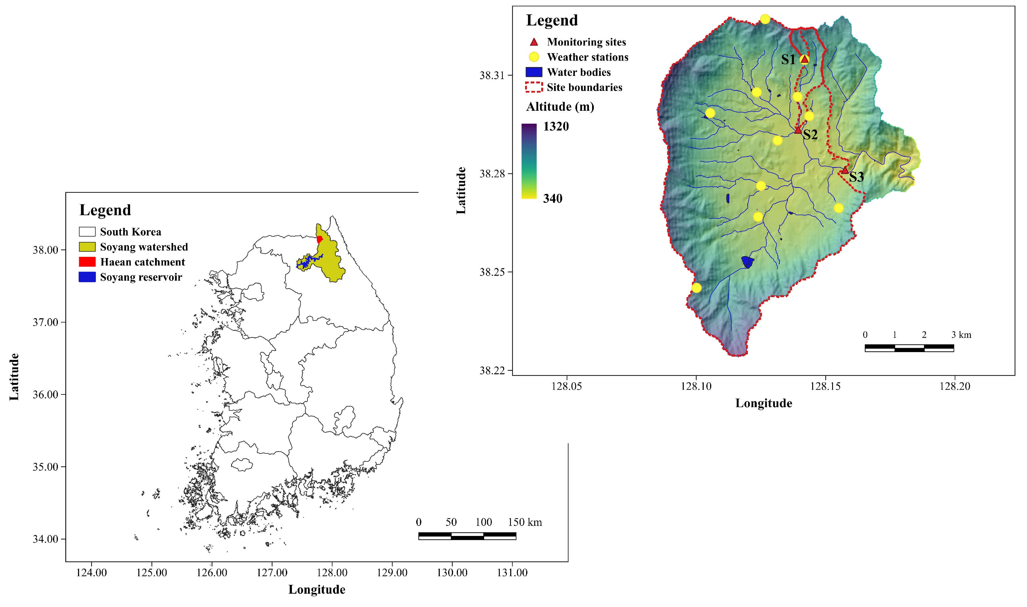
Figure 1. General description of the study area. Locations of the Soyang lake watershed and Haean catchment in South Korea are described in the lower left figure. In the upper right figure, the topography and stream networks of the study area, with the monitoring sites (red triangles) and weather stations (yellow circles) used for the DMMF model are presented.
Water 11 00957 g001
Figure 2. Schematic hydrological phase of the DMMF model (modified from Figure 3 of Choi et al. [15]).
Water 11 00957 g002
Figure 3. Schematic sediment phase of the DMMF model (modified from Figure 4 of Choi et al. [15]).
Water 11 00957 g003
Figure 4. Represented soil class from a 2009 catchment-wide field survey from the TERRECO project.
Water 11 00957 g004
Figure 5. LULC classes and their spatial configurations for the Haean catchment in the year 2010 [35].
Water 11 00957 g005
Figure 6. Calibration (S1 and S2) and validation (S3) result for stream discharge, and suspended sediment measured at the outlet of each sub-catchment.
Water 11 00957 g006
Figure 7. (a) Annual net soil erosion ( t / h a / year ) of the entire Haean catchment and (b) soil erosion class according to the soil erosion risk categories from OECD [69,70].
Water 11 00957 g007
Figure 8. Total annual sediment yields entering the stream (upper panel) and sediment yield reduction efficiency per unit conversion area (lower panel) through changing bare soil and crop fields into forest sequentially from the area with the highest to the area with the lowest amount of net soil erosion ( S L n e t ), sediment inflow to the element ( S L i n ), and sediment output from the element ( S L o u t ).
Water 11 00957 g008
Table 1. Input parameters of the daily based Morgan–Morgan–Finney (DMMF) model (modified from Table 1 of Choi et al. [15])
TypeParameterDescriptionUnit
TopographySSlope angle( rad )
r e s Grid size of a raster map( m )
ClimateRDaily rainfall(mm/day)
R I Mean rainfall intensity of a day( mm / h )
E T Daily evapotranspiration(mm/day)
Soil P c Proportion of clay in the surface soil(proportion)
P z Proportion of silt in the surface soil(proportion)
P s Proportion of sand in the surface soil(proportion)
S D Soil depth( m )
θ i n i t Initial soil water content of the entire soil profile( vol / vol )
θ s a t Saturated water content of the entire soil profile( vol / vol )
θ f c Soil water content at field capacity of the entire soil profile( vol / vol )
KSaturated soil lateral hydraulic conductivity of the entire soil profile(mm/day)
D K c Detachability of clay particles by rainfall( g / J )
D K z Detachability of silt particles by rainfall( g / J )
D K s Detachability of sand particles by rainfall( g / J )
D R c Detachability of clay particles by surface runoff( g / mm )
D R z Detachability of silt particles by surface runoff( g / mm )
D R s Detachability of sand particles by surface runoff( g / mm )
LULC P I Area proportion of the permanent interception of rainfall(proportion)
I M P Area proportion of the impervious ground cover(proportion)
G C Area proportion of the pervious ground cover of the soil surface(proportion)
C C Area proportion of the canopy cover of the soil surface(proportion)
P H Average height of vegetation or crop cover( m )
DAverage diameter of individual plant elements at the surface( m )
N V Number of individual plant elements per unit area( number / m 2 )
d a Typical flow depth of surface runoff( m )
nManning’s roughness coefficient of the soil surface( s / m 1 / 3 )
Table 2. Typical soil characteristics of each represented soil class of the Haean catchment from a 2009 catchment-wide field survey from TERRECO project.
Classification SD P c P z P s θ sat * θ fc *K *
Very steep forest2.550.170.330.500.47 (0.41–0.53)0.21 (0.06–0.31)1.97 (0.63–4.55)
Forest4.380.220.350.430.45 (0.41–0.54)0.17 (0.06–0.33)2.18 (0.63–4.55)
Moderate to steep dry field2.180.080.290.640.36 (0.34–0.39)0.18 (0.17–0.20)0.33 (0.18–0.66)
Flat dry field4.850.030.150.820.36 (0.34–0.41)0.18 (0.08–0.25)0.49 (0.09–2.25)
Rice paddy1.600.070.320.620.37 (0.36–0.39)0.16 (0.14–0.18)0.50 (0.41–0.72)
Sealed ground2.001.000.000.00---
* θsat, θfc, and K were estimated with the model ROSETTA Lite v.1.1 [44]. The numbers in parentheses indicate the range of values of soil layers that constitute each represented soil class.
Table 3. The initial parameter settings for each LULC class.
LULCLeaf-out ( a ) (Planting)Leaf-fall ( a ) (Harvest) PI ( b ) IMP ( c ) GC ( d ) CC max ( e ) PH ( f ) D ( g ) NV ( h ) d a ( i ) n ( j )
Forest1123070.200.001.000.9530.02.000.600.1000.20
Semi-natural1123070.300.001.000.950.500.015000.1000.20
Shrub1123070.200.000.300.950.500.12200.1000.20
Rice paddy1362830.300.001.00 (0.00)0.801.000.042000.0500.10
Potato1202430.120.50 (0.00)0.00 (0.26)0.710.450.106.000.1500.10
Bean1473040.200.50 (0.50)0.00 (0.58)0.890.700.026.000.1500.10
Radish1532350.150.50 (0.25)0.00 (0.14)0.640.480.066.000.1500.10
Cabbage1402010.250.50 (0.50)0.00 (0.31)0.850.550.203.640.1500.10
Other dry crops1203040.180.50 (0.31)0.00 (0.32)0.770.570.105.320.1500.10
Orchard1203030.250.000.400.954.001.500.160.0500.10
Ginseng *1232980.200.000.501.001.300.0137.50.4000.20
Bare soil--0.000.000.000.000.000.000.000.0500.01
Urban--0.001.000.000.000.000.000.000.0050.01
( a ) Typical leaf-out and leaf-fall dates of each LULC were presented as day of the year (DOY). For annual crops, the dates represented the typical planting and harvest date of each crop [30]; ( b ) The reference values from Morgan and Duzant [40] were used for the area proportion of the permanent interception of rainfall ( P I ) for each LULC type; ( c ) I M P for dry fields are different between cultivation and non-cultivation periods. Values in parentheses represent I M P for non-cultivation periods; ( d ) G C for dry fields is different before and after harvest. After harvest, crop residues and weeds remained as the ground cover of dry fields, according to dry crop data, from the field campaign of the TERRECO project in 2009. G C for rice paddy in cultivation season was set to one reflecting water-filled condition that protected the surface from erosion; ( e ) Because C C values varied with time, we made a list of maximum C C ( C C m a x ). Semi-natural, shrub, and ginseng utilize fixed reference values from Morgan and Duzant [40]; ( f ) We used fixed reference P H values from Morgan and Duzant [40] for LULCs of other than dry crops. Maximum P H values for dry crops were listed from the field measurement data varying with time; ( g ) We used fixed reference D values from Morgan and Duzant [40] for LULCs of other than dry crops. D values for dry crops utilized typical crop characteristics from Rural Development Administration of South Korea [48]; ( h ) We used reference N V values from Morgan and Duzant [40] for LULCs of other than dry crops and ginseng. N V values which were estimated from the field measurement data and Rural Development Administration of South Korea [48] were used for dry crops and ginseng, respectively; ( i ) We assumed shallow rill condition for forest, semi-natural and shrub, and assumed unchannelled flow condition for bare soil, rice paddy, and orchard using values presented in Morgan and Duzant [40]. d a values for other LULCs derived from furrow heights of the fields, using field measurement data for dry crops and data from the Rural Development Administration of South Korea [48] for ginseng; ( j ) According to the guide values for Manning’s n from Morgan [49], the values of n for natural land covers (i.e., forest, semi-natural, and shrub), crop fields, ginseng, and smooth surfaces (bare soil and urban) are 0.2, 0.1, 0.2, and 0.01, referring to natural range land, average tillage conditions, wheat mulching, and smooth bare soil or asphalt conditions, respectively; * The permeable black awning screen is generally installed 1.3 m above the ginseng field [48], and it acts as a plant canopy. Therefore, the cover ratio of the screen in the field and height of the screen is utilized for canopy cover ( C C ) and plant height ( P H ) values for ginseng.
Table 4. Soil erosion risk categories defined by OECD [69,70].
Erosion ClassTolerableLowModerateHighSevere
Soil erosion rate ( t / h a / year )<66–10.911–21.922–32.9>33
Table 5. List of important parameters from forested site with Sobol’ index greater than 0.05 for stream discharge ( S I Q ) and suspended sediment to the stream ( S I S L ), and their optimized values from the DE algorithm.
ParametersSoil Class/LULC SI Q SI SL Optimized Values
θ f c Forest soil0.0350.1182.24 × 10−1
KForest soil0.2020.0826.17 × 101
D R c Forest soil00.2132.25 × 10−1
P I Forest0.7810.1806.66 × 10−5
G C Forest00.7759.92 × 10−1
d a Forest00.1447.77 × 10−3
Table 6. List of important parameters ( S I > 0.05) for stream discharge ( S I Q ) and suspended sediment ( S I S L ), and their optimized values from DE algorithm.
ParametersSoil Class/LULC SI Q SI SL Optimized Values
θ f c Moderate to steep dry field soil0.1150.1123.18 × 10−1
KModerate to steep dry field soil0.2230.0206.06 × 10−1
KFlat dry field soil0.0620.0011.59 × 10−1
D R c Moderate to steep dry field soil00.2171.39
D R z Moderate to steep dry field soil00.1199.59 × 10−1
P I Semi-natural0.2520.0484.16 × 10−4
P I Rice paddy0.1010.0002.91 × 10−1
P I Other dry crops0.1780.0111.28 × 10−4
G C Semi-natural00.0803.60 × 10−2
d a Semi-natural00.1581.74 × 10−1
d a Bean00.1052.93 × 10−1
α ---1.75 × 10⁻²
β ---4.57 × 10⁻²
Table 7. Mean annual net soil erosion rate ( t / h a / year ) and mean slope of each LULC type.
LULCMean Annual Net Soil Erosion Rate (t/ha/year)Mean Slope (°)
Bare soil997.809.8
Bean763.827.6
Ginseng388.838.5
Potato357.607.9
Radish310.068.4
Other dry crops294.238.4
Semi-natural126.349.0
Shrub105.5411.1
Cabbage79.307.6
Catchment average52.6816.0
Forest−75.2522.0
Rice paddy−171.833.0
Orchard−227.148.1
Urban−284.716.0