Allocating Water Environmental Capacity to Meet Water Quality Control by Considering Both Point and Non-Point Source Pollution Using a Mathematical Model: Tidal River Network Case Study

Abstract
:1. Introduction
2. Methods of Total Pollutant Distribution
2.1. Optimization Assignment Model
- (1)
- The upper limit value of decision variables (), which was the maximum allowed discharged quantity, was set according to the current emission characteristics of pollution sources, with reference to compulsive administrative requirements set by the local government for pollutant discharge reduction, comprehensively considering local economic, social, and environmental sustainability, and so on.
- (2)
- The lower limit value of decision variables (), which was the maximum cost efficiency and technical feasibility of the discharged quantity, was set according to the current emission characteristics of pollution sources, combined with the existing level of pollution treatment technology and disposal cost control.
2.2. Point Source and Non-Point Source Response Coefficients for Contaminant Concentration in the Control Section
2.3. Solving the Optimization Model Method
- (1)
- Set operating parameters. The parameters involved in the genetic algorithm included: population size, ; mutation probability, ; crossover probability, ; and evolution algebra, . The different values of the parameters will directly affect the performance of the algorithm, so multiple debuggings should be performed, and the best value should be selected after comparison. In this case, the population size was 100, the crossover probability was 0.001, and the evolution algebra was 100.
- (2)
- Generate the initial population. Several individuals were randomly selected and judged according to the constraints, and the individuals who met the conditions as a whole constituted the initial population.
- (3)
- Fitness and choice. According to the principle of natural selection, individuals with high fitness are inherited to the next generation. The objective function value was generally used as the individual fitness.
- (4)
- Crossover. In genetic algorithms, crossover is mainly used to generate new individuals. The object of operation change was the binary code of the decision variable, not the decision variable itself. Firstly, individuals were selected and paired randomly according to a certain method. Then, the location of the intersection and exchange of genes, according to a certain crossover method, are determined to reflect the idea of information exchange. Since the new individual obtained after the intersection was not necessarily a feasible solution, the result was checked by constraint conditions. If the condition remained unsatisfied, the crossover operation was performed again until the constraint condition was satisfied or the number of crossover operations reached the limit value.
- (5)
- Mutation. The mutated object was also the binary code of the decision variable. The mutation here only required the individual to reverse the value at the mutation point (0 to 1 and 1 to 0). Variation is the main method of generating new individuals, but new individuals after mutation required testing by constraints.
- (6)
- Generate a new generation of populations. From the offspring generated by crossover and mutation, individuals were selected as parents to generate a new population generation. In general, the optimal individuals in each generation were selected to be inherited to the next generation. Therefore, the solution of the model can be obtained by decoding the best individual of the last generation.
3. Case Study
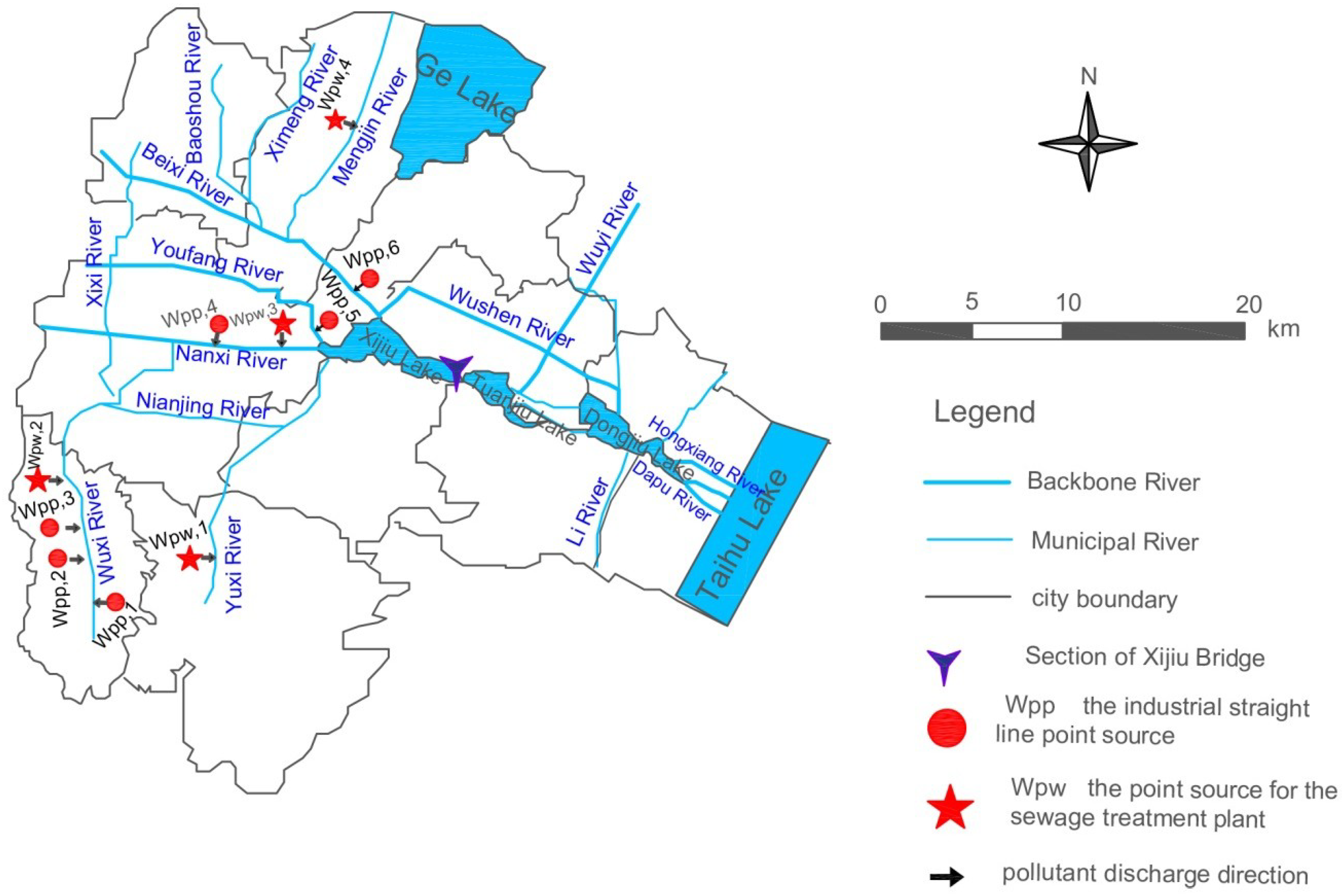
3.1. Research Area
3.2. Establishing the Hydrodynamic Model of the River Network Considering Rainfall and Runoff
3.2.1. Boundary Conditions
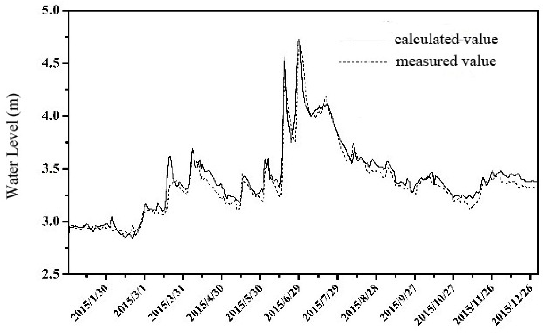
3.2.2. Parameter Values and Water Model Validation
3.3. Establishing the River Network Water Quality Model Based on Time Variation of Non-Point Source Release into Rivers
3.3.1. Boundary Conditions
3.3.2. Point Source and Non-Point Source Generalization
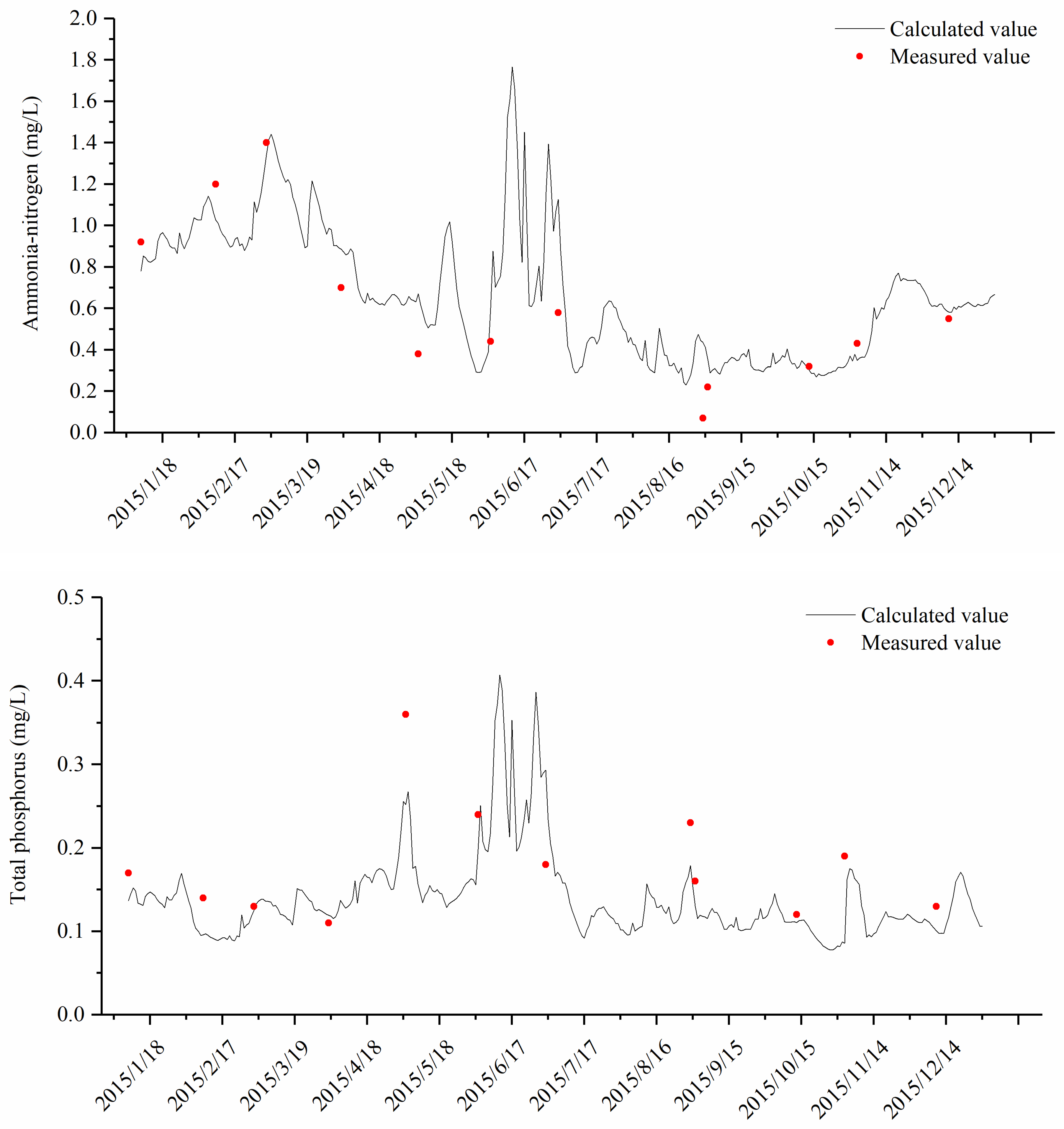
3.3.3. Parameter Value and Model Validation
3.4. Constructing an Optimal Allocation Model for Total Pollutants Based on Controlled Section Water Quality Standards, Considering the Synergetic Influence of Point and Non-Point Sources
3.5. Total Pollutant Distribution Results
3.6. Feasibility Analysis
4. Discussion and Conclusions
- (1)
- The analysis results showed that when the maximum allowable emission of each pollutant discharge port was inputted into the model, the annual numbers of days for ammonia-nitrogen and total phosphorus meeting the standard were 334 and 332 days, respectively, and the water quality compliance rates of the control section was 91.5% and 91%, respectively. The ammonia-nitrogen and total phosphorus concentrations in the controlled section achieved class III water quality targets for 90% of the year. These all meet the water quality compliance rate requirements of the control section.
- (2)
- The method systematically and intuitively reflects the feasibility of optimizing allocation results of the total amount. It overcomes the shortcomings in the feasibility of optimizing the distribution method, solves the key constraints in its application, and provides effective and reliable technical support for the control and management of regional total pollutants based on water quality improvement. It offers improvement for environment management and protection.
Author Contributions
Funding
Conflicts of Interest
References
- Zhang, L.K. Study on Total Quantity Control Technology of Ashi River Basin Based on Nonpoint Source Pollution Control. Master’s Thesis, Chinese Academy of Environmental Sciences, Beijing, China, 2014. [Google Scholar]
- Chen, L.; Han, L.; Tan, J.; Zhou, M.; Sun, M.; Zhang, Y.; Chen, B.; Wang, C.; Liu, Z.; Fan, Y. Water Environmental Capacity Calculated Based on Point and Non-Point Source Pollution Emission Intensity under Water Quality Assurance Rates in a Tidal River Network Area. Int. J. Environ. Res. Public Health 2019, 16, 428. [Google Scholar] [CrossRef] [PubMed]
- Zheng, X.Y.; Zhu, J.D.; Zhu, W.B. Research on water environmental capacity of dynamic river system. Adv. Water Sci. 1997, 8, 25–31. [Google Scholar]
- Han, L.; Lu, D.; Ji, H. Study on the Concentration Response of Pollutant Concentration in the Inflow and Outflow Section of the Cross-type Mouth of Plain River Network. J. Sun Yat-Sen Univ. (Nat. Sci. Ed.) 2011, 50, 123–128. [Google Scholar]
- Han, L.; Lu, D. Prospect of numerical simulation study on water quality of plain river network. J. Hohai Univ. (Nat. Sci. Ed.) 2004, 32, 127–130. [Google Scholar]
- Yao, Y.J.; Yin, H.L.; Li, S.I. The computation approach for water environmental capacity in tidal river network. J. Hydrodyn. 2006, 18, 269–273. [Google Scholar] [CrossRef]
- Bian, B.; Zhu, W.; Li, B. The characteristics of non-point source pollution and its control techniques in western Taihu Basin. Water Resour. Prot. 2015, 31, 48–55. [Google Scholar]
- Dong, Y. Study on Coupling Simulation and Control Strategy of Non-Point Source Pollution in Dianchi Lake between Urban and Rural Areas; Tsinghua University: Beijing, China, 2016. [Google Scholar]
- Zhang, L. Study on Water Pollutant Total Amount Control Technique in ASHI River Basin Based on Non-Point Source Pollution Control; Chinese Research Academy of Environmental Sciences: Beijing, China, 2014. [Google Scholar]
- Wang, C.Y.; Peng, H.; Zhang, S.W. Water Pollution Control Plan TMDL Project on Wuhan East Lake. People’s Yangtze River 2010, 41, 86–89. [Google Scholar]
- Bao, K.; Feng, Y.; Sun, H. Research on Calculation Method of Water Environmental Capacity Based on Water Quality Control at Control Section—Taking Yincun Port as an Example. Resour. Sci. 2011, 33, 249–252. [Google Scholar]
- Wang, Z.X.; Pang, Y.; Luo, J. Study on Water Environment Capacity and Water Quality Control Plan for Plain River Network in Dianshan Lake Basin. J. Water Resour. Water Eng. 2015, 12, 249–252. [Google Scholar]
- Ma, X. Water Environmental Capacity Calculation and Allocation Based on the Optimal Reduction Model of Pollution; Tsinghua University: Beijing, China, 2017. [Google Scholar]
- Li, R.Z.; Qian, J.Z.; Wang, J.Q. Research on the Total Allocation of Water Pollutants Allowed Emissions. J. Hydraul. Eng. 2003, 5, 112–115. [Google Scholar]
- Xu, H.; Wu, J.M.; Zhao, P.D. Case studies on sustainability assessment of urban wetland resources. Fresenius Environ. Bull. 2013, 22, 3458–3464. [Google Scholar]
- Chen, D.J.; Lv, J.; Shen, Y.N. Water Environment Gini Coefficient Method for Multi-objective Fair Allocation of Water Environment Capacity among Regions. Environ. Pollut. Prev. 2010, 32, 88–91. [Google Scholar]
- Wang, L.; Zhang, H.W.; Yue, L. Research on the Model of Optimizing Distribution of Total Water Pollutant Industry. Environ. Sci. 2005, 26, 195–198. [Google Scholar]
- Wang, J.N.; Pan, X.Z. Application of Linear Programming Method in Allocation of Environmental Capacity Resources. Environ. Sci. 2005, 26, 195–198. [Google Scholar]
- Xun, F.F.; Ge, Y.J.; Ma, J.Y. Application of Linear Programming in Water Environment Capacity Calculation. J. Water Resour. Water Eng. 2009, 20, 180–182. [Google Scholar]
- Dong, Y.B.; Zhang, H.X.; Li, Z.W. Study on Water Environment Capacity of Taizihe Liaoyang Section Based on Linear Programming. Water Conserv. Technol. Econ. 2016, 22, 12–14. [Google Scholar]
- Wu, S.Y.; Hu, C. Research on water environment capacity of the Weihe River system based on the water ecological function zoning. J. Meteorol. Environ. 2014, 30, 107–111. [Google Scholar]
- Wan, J.M.; Li, S.Y. Research on Total Control Scheme of Water Environmental Capacity in Tidal River Reaches. Environ. Sci. Manag. 2009, 34, 34–36. [Google Scholar]
- Jing, H.X.; Li, X.B.; Fang, H.Y.; Liu, C.G. Investigation of the river water environment capacity allocation by using linear programming model. J. Water Resour. Water Eng. 2018, 29, 34–38. [Google Scholar]
- Li, M. Study on Estimation and Allocation Method of River Water Environmental Capacity for Liaohe River in Tieling; Shenyang Ligong University: Shenyang, China, 2011. [Google Scholar]
- Deng, Y.X.; Meng, W.; Zheng, B.H.; Fu, G.; Lei, K. Application of linear programming method based on response fields in total load allocation for Yangtze estuary and adjacent sea. Res. Environ. Sci. 2009, 16, 995–1000. [Google Scholar]
- Holland, J. Adaptation in Natural and Artificial Systems; University of Michigan Press: Ann Arbor, MI, USA, 1975. [Google Scholar]
- Yuan, X.M.; Li, H.Y.; Li, S.K. Application of Neural Network and Genetic Algorithm in Water Science; China Water Conservancy and Hydropower Press: Beijing, China, 2002. [Google Scholar]
- Xu, L.N.; Li, L.L. Application of Genetic Algorithm in Nonlinear System Identification. J. Harbin Inst. Technol. 1999, 31, 39–42. [Google Scholar]
- Ozemir, O.N.; Ucaner, E. Validation of genetic algorithms for the hydraulic calibration of a water supply network. Fresenius Environ. Bull. 2007, 16, 278–284. [Google Scholar]


| Pollutant Source | Discharge Load (t/year) | Pollutant Source Style | |
|---|---|---|---|
| Ammonia-Nitrogen (NH3-N) | Total Phosphorus (TP) | ||
| WPP,1 | 2.2 | 0.2 | Point source industrial outlet |
| WPP,2 | 2 | 0.2 | |
| WPP,3 | 1.3 | 0.1 | |
| WPP,4 | 0.2 | 0 | |
| WPP,5 | 0.2 | 0 | |
| WPP,6 | 0.1 | 0 | |
| WPW,1 | 30.3 | 6.06 | Point source waste water treatment outlet |
| WPW,2 | 10.4 | 2.08 | |
| WPW,3 | 8.03 | 1.6 | |
| WPW,4 | 7.3 | 1.46 | |
| WNS,1 | 20.1 | 2.5 | Non-point source |
| WNS,2 | 45.6 | 5.7 | |
| WNS,3 | 65.3 | 8.2 | |
| WNS,4 | 32.4 | 4 | |
| WNS,5 | 18.6 | 2.3 | |
| WNS,6 | 10.7 | 1.4 | |
| WNS,7 | 11.1 | 1.4 | |
| WNN,1 | 37.2 | 7.99 | Non-point source agricultural |
| WNN,2 | 35.5 | 7.77 | |
| WNN,3 | 67.9 | 39.7 | |
| WNN,4 | 61.2 | 13.3 | |
| WNN,5 | 30.7 | 6.62 | |
| WNN,6 | 43.7 | 9.7 | |
| WNN,7 | 9.81 | 1.95 | |
| Total | 551.7 | 124.2 | |
| Index | Value | Governance Measures |
|---|---|---|
| 10% | Takeover or build a decentralized wastewater treatment facility | |
| 40% | According to relevant pollution control management requirements | |
| 20% | Various measures related to agriculture | |
| 100% | Current pollution-free control management requirements | |
| 60% | Accelerate the upgrading of urban sewage treatment plants | |
| 80% | Multi-channel utilization of tail water | |
| 80% | Enterprises in industrial concentration areas takeover, printing and dyeing enterprises raise standards, and the reuse of water is increased |
| Pollutant Source Code | NH3-N | TP | ||||||
|---|---|---|---|---|---|---|---|---|
| Current Pollution Load | Allowed Emissions | Reduction | Reduction Rate | Current Pollution Load | Allowed Emissions | Reduction | Reduction Rate | |
| Unit | (t/year) | (t/year) | (t/year) | (%) | (t/year) | (t/year) | (t/year) | (%) |
| WPP,1 | 2.2 | 1.15 | 1.05 | 48 | 0.2 | 0.1 | 0.1 | 50 |
| WPP,2 | 2 | 1.04 | 0.96 | 48 | 0.2 | 0.11 | 0.09 | 47 |
| WPP,3 | 1.3 | 0.68 | 0.62 | 48 | 0.1 | 0.05 | 0.05 | 51 |
| WPP,4 | 0.2 | 0.1 | 0.1 | 52 | 0 | 0 | 0 | 0 |
| WPP,5 | 0.2 | 0.1 | 0.1 | 50 | 0 | 0 | 0 | 0 |
| WPP,6 | 0.1 | 0.1 | 0 | 0 | 0 | 0 | 0 | 0 |
| WPW,1 | 30.3 | 21.8 | 8.46 | 28 | 6.06 | 4.87 | 1.19 | 20 |
| WPW,2 | 10.4 | 7.3 | 3.1 | 30 | 2.08 | 1.62 | 0.46 | 22 |
| WPW,3 | 8.03 | 5.65 | 2.38 | 30 | 1.6 | 1.28 | 0.32 | 20 |
| WPW,4 | 7.3 | 5.13 | 2.17 | 30 | 1.46 | 1.17 | 0.29 | 20 |
| WNS,1 | 20.1 | 3.63 | 16.5 | 82 | 2.5 | 1.5 | 1 | 40 |
| WNS,2 | 45.6 | 8.71 | 36.9 | 81 | 5.7 | 3.4 | 2.3 | 40 |
| WNS,3 | 65.3 | 12.2 | 53.1 | 81 | 8.2 | 5.18 | 3.02 | 37 |
| WNS,4 | 32.4 | 5.77 | 26.6 | 82 | 4 | 2.27 | 1.73 | 43 |
| WNS,5 | 18.6 | 3.37 | 15.2 | 82 | 2.3 | 1.33 | 0.97 | 42 |
| WNS,6 | 10.7 | 1.87 | 8.83 | 82 | 1.4 | 0.79 | 0.61 | 44 |
| WNS,7 | 11.1 | 1.97 | 9.13 | 82 | 1.4 | 0.79 | 0.61 | 44 |
| WNN,1 | 37.2 | 16.6 | 20.7 | 56 | 7.99 | 6.33 | 1.66 | 21 |
| WNN,2 | 35.5 | 14.9 | 20.5 | 58 | 7.77 | 4.65 | 3.12 | 40 |
| WNN,3 | 67.9 | 21.6 | 46.3 | 68 | 39.7 | 16.2 | 23.6 | 59 |
| WNN,4 | 61.2 | 21 | 40.2 | 66 | 13.3 | 9.52 | 3.74 | 28 |
| WNN,5 | 30.7 | 15.7 | 15 | 49 | 6.62 | 4.48 | 2.14 | 32 |
| WNN,6 | 43.7 | 17.7 | 26 | 60 | 9.7 | 6.18 | 3.51 | 36 |
| WNN,7 | 9.81 | 7.23 | 2.58 | 26 | 1.95 | 1.26 | 0.7 | 36 |
| Total | 551.7 | 195.2 | 356.5 | 65 | 124.2 | 73.02 | 51.18 | 41 |
© 2019 by the authors. Licensee MDPI, Basel, Switzerland. This article is an open access article distributed under the terms and conditions of the Creative Commons Attribution (CC BY) license (http://creativecommons.org/licenses/by/4.0/).
Share and Cite
Chen, L.; Han, L.; Ling, H.; Wu, J.; Tan, J.; Chen, B.; Zhang, F.; Liu, Z.; Fan, Y.; Zhou, M.; et al. Allocating Water Environmental Capacity to Meet Water Quality Control by Considering Both Point and Non-Point Source Pollution Using a Mathematical Model: Tidal River Network Case Study. Water 2019, 11, 900. https://doi.org/10.3390/w11050900
Chen L, Han L, Ling H, Wu J, Tan J, Chen B, Zhang F, Liu Z, Fan Y, Zhou M, et al. Allocating Water Environmental Capacity to Meet Water Quality Control by Considering Both Point and Non-Point Source Pollution Using a Mathematical Model: Tidal River Network Case Study. Water. 2019; 11(5):900. https://doi.org/10.3390/w11050900
Chicago/Turabian StyleChen, Lina, Longxi Han, Hong Ling, Junfeng Wu, Junyi Tan, Bo Chen, Fangxiu Zhang, Zixin Liu, Yubo Fan, Mengtian Zhou, and et al. 2019. "Allocating Water Environmental Capacity to Meet Water Quality Control by Considering Both Point and Non-Point Source Pollution Using a Mathematical Model: Tidal River Network Case Study" Water 11, no. 5: 900. https://doi.org/10.3390/w11050900
APA StyleChen, L., Han, L., Ling, H., Wu, J., Tan, J., Chen, B., Zhang, F., Liu, Z., Fan, Y., Zhou, M., & Lin, Y. (2019). Allocating Water Environmental Capacity to Meet Water Quality Control by Considering Both Point and Non-Point Source Pollution Using a Mathematical Model: Tidal River Network Case Study. Water, 11(5), 900. https://doi.org/10.3390/w11050900