1. Introduction
In the planning and management of urban water systems, the temporal and spatial variability of residential water demand is one of the most influential sources of uncertainty [
1,
2]. Conventional modelling approaches often neglect this aspect, by involving on the one hand, identical multiplier patterns to provide a coarse representation of the diurnal variation of water demand (typically from hour-to-hour) and on the other hand, simplified allocation techniques to express the variation of demand across different points (e.g., nodes) of the network. Despite its practical simplicity, this approach fails to capture adequately the high spatio-temporal variability and uncertainty of water demand (e.g., [
3,
4,
5,
6,
7]), which becomes more and more intense as the scales of analysis become lower [
8]. Furthermore, such a modelling concept does not allow the design, evaluation and management of water distribution systems (WDS) within an uncertainty-aware framework since it implies the use of deterministic water demand patterns as inputs in, typically, deterministic simulation models. A way to address some of these shortcomings, is the study, analysis and modelling of the uncertain nature of water demand in a probabilistic framework by treating the latter as a stochastic process. In essence, this allows the development of stochastic water demand forecasting tools (e.g., see [
9,
10,
11,
12] and the references herein) and simulation methodologies. In this work, we focus on simulation that allows the generation of an arbitrarily large number of synthetic, yet statistical consistent, realizations of water demand events, which can then serve as non-deterministic inputs to a WDS, allowing for the probabilistic assessment of its performance under different input scenarios.
During the last decades, the rising deployment of smart metering systems provided new modelling perspectives by delivering large amounts of detailed water demand measurements (e.g., [
13,
14,
15]). Taking advantage of this dataflow, the research community focused on the modelling of residential water demand at very fine temporal (down to 1 s) and spatial (i.e., household or even water appliance) scales. Then, when necessary, synthetic records at higher levels can be derived via a bottom-up approach that involves the aggregation of fine-resolution data [
2].
As literature reveals, the notion of the rectangular pulse has prevailed in the stochastic modelling of residential water demand. This may be associated with an attempt to provide a physical realism in the representation of the real process. In effect, this mechanism, studied at a micro-scale level, can be regarded as a sequence of individual or clustered pulses (events) with constant duration and intensity. Stochastic simulation techniques, such as the Poisson rectangular pulse (PRP) processes [
16,
17,
18,
19,
20,
21,
22,
23] and Poisson-cluster processes, i.e., the Neyman–Scott [
24,
25,
26] and Bartlett–Lewis [
27] mechanisms, have been employed to generate synthetic water demand events, which occur at continuous time, at the level of a single-household or group of households. Moving from continuous to discrete-time processes, the aggregated demand series can be obtained by summing up all pulses which are active in each discrete time interval. Furthermore, simulation schemes, both stochastic and deterministic, that produce demand signals starting from the level of individual micro-components (i.e., water appliances and uses) have also been developed [
28,
29,
30,
31].
The above models, and especially PRP and appliance-based schemes, focus mainly on the generation of pulses, whose characteristics (frequency, intensity, duration) are statistically consistent with those of the observed demand events. This is also implied by the adopted procedures for the estimation of their parameters. More specifically, the structure of PRP, implying a one-to-one correspondence between a pulse and an event, allows the fitting of the underlying model’s distributions of pulse characteristics directly upon the observed events, if instantaneous demand measurements (e.g., 1-sec time resolution) are available [
16,
17,
18,
20,
21,
22]. The schemes based on the simulation of micro-components provide a detailed and elegant description of the real water demand mechanism, but their proper parameterisation is a difficult task since it requires deep knowledge of the consumption habits of the users and the characteristics of water usage [
23,
32,
33].
However, typical WDS modelling applications require demand records across a wide range of higher temporal and spatial levels where the characteristics of individual events are no longer identifiable (e.g., [
32]). Thus, from a practical point-of-view, in real-world applications, apart from those that explicitly focus on the influence of individual uses at a micro-scale level (see e.g., [
28,
34,
35]), the key task is not the modelling of individual demand events
per se, but the adequate reproduction of the statistical and stochastic properties of the discrete-time demand process at different temporal (e.g., 1 min or 15 min scale etc.) and spatial (e.g., household, group of various number of users, nodes etc.) levels. The above mentioned models, though fitted on the basis of individual pulse characteristics, essentially embrace this necessity since their evaluation is also conducted upon statistical parameters of the aggregated demand series which are typically involved in the WDS applications (i.e., main summary statistics or cumulative distribution function of demand, water volume per day, maximum flow at different time scales and probability of no demand).
These models can be regarded as
implicit methods in terms of reproducing the marginal and dependence characteristics (i.e., the stochastic structure) of the discrete-time water demand process, implying that this reproduction can be achieved via an adequate representation of the characteristics of individual events. In fact, empirical evidence suggests that they provide a satisfactory, though not explicit, approximation of some statistical parameters of the observed aggregated series. The performance and effectiveness of these models is closely associated with the availability of super-fine observed data that allow the decomposition of demand measurements into single equivalent pulses with identifiable characteristics (see e.g., [
16,
36]). However, such data can be typically found only at a small number of pilot households, while the commercially available energy-efficient, cost-effective and with long lifetime smart metering devices provide water demand records with higher time step (i.e., 1 min or higher).
Another parameterisation approach, with direct reference to the discrete-time process, consists in obtaining the parameters of PRP and Poisson-cluster models so as to preserve specific properties of the aggregated demand series. Since this approach does not require data at the level of individual pulses, it can be also applied when data of larger time step are available. This method has been used to fit the original PRP model [
19], and is the standard parameterisation procedure for the Poisson-cluster processes [
24,
27]. The structure of the latter (i.e., each event is formulated by a cluster of pulses) does not allow to obtain the parameters directly from the characteristics of observed events. This approach typically involves the theoretical equations of the models which express the main statistical properties (i.e., first- and second-order moments and the probability of no demand) of the discrete-time aggregated process as a function of model parameters, while numerical schemes in cases where the analytical expressions are not available (e.g., PRP model with correlated pulse intensity and duration) have also been studied [
22]. Using this concept, pulse-based models are able to generate synthetic water demand data that explicitly reproduce specific properties of the observed aggregated series. However, these are limited to low-order summary statistics (i.e., mean, variance and probability of no demand) regarding the marginal properties of the process and lag-1 autocorrelation coefficient regarding its dependence structure. In this regard, the problem of stochastic simulation of residential water demand is partially addressed since neither the complete marginal distribution nor the whole stochastic structure of the process are explicitly preserved. This also stands for the models which are fitted upon pulse characteristics where the aggregated series are derived implicitly.
Further to the models based on the notion of pulse, a limited number of alternative stochastic procedures for the simulation of water demand process can be found in the literature. More specifically, Gargano et al. [
32] proposed a method for the probabilistic representation of the daily trend of residential water demand for different number of users, using a mixed-type distribution to describe the whole process without, however, accounting for the underlying temporal dependences. Alvisi et al. [
37,
38], using a bottom-up approach, employed random polynomial processes along with reordering techniques to enable the generation of synthetic water demand data which are statistically consistent (in terms of mean, variance and spatio-temporal correlations) with observed the time series at lower and higher spatial and temporal scales. Following the opposite procedure (i.e., top-down allocation), stochastic disaggregation methods, typically applied in the field of hydrology, have also been used to allocate, probabilistically, total amounts of water of an area to its enclosed nodes [
6]. Furthermore, and though not proposing stochastic simulation models, it is worth to mention the work of Kossieris and Makropoulos [
39] who study the statistical and distributional properties of residential water demand at various scales, as well as the study of Gargano et al. [
40] on the evaluation of probabilistic models to describe the peak residential water demand. Lastly, Magini et al. [
8,
41] and Vertommen et al. [
42] studied the scaling properties of water demand at different spatial and temporal levels, while recently Magini et al. [
43] employed those properties to generate large number of scenarios of spatially correlated demand series at the node of a network.
In WDS modelling, the adequate reproduction of these two aspects, i.e., the marginal distribution and stochastic structure, of the discrete-time water demand process at different temporal and spatial scales is of high importance. Regarding the first, the probabilistic behaviour of a process is fully described by its marginal distribution. On the contrary, low-order statistics provide only a part of the picture, without explicitly accounting for other important aspects of the marginal properties such as tail behaviour and hence the reproduction of extremes. This is crucial especially in the design of WDS that requires a proper characterisation of peak flows at different temporal resolutions (e.g., [
2,
40,
44]). This is further highlighted in the work of Kossieris and Makropoulos [
39] who demonstrate that the use of some low-order moments (i.e., up to third moment) is not sufficient, since different distributions, having the same moments, result in totally different behaviour in terms of maximum water demands. Additionally, a complete description of the statistical behaviour (e.g., in terms of marginal distribution) of residential water demand is also important in WDS quality modelling applications where different flows, further to maximum values, are used in hydraulic models (e.g., see [
3] and references herein).
The importance of appropriately reproducing the temporal and spatial dependencies, i.e., stochastic structure, encountered in water demand process has also been highlighted by many researchers [
3,
4,
5,
6,
7,
24,
37,
38,
45,
46]. More specifically, autocorrelation structure expresses the dynamics of water demand process in time, affecting many parameters in the modelling of WDS, e.g., peak flows, stagnation time, velocities in the pipes, restoration time after pipe breaks etc (e.g., see [
37] and references herein). On the other hand, cross-correlation expresses how water demands co-vary across different nodes of the network, and it is also associated with many aspects of the system, e.g., system’s performance on the basis of the main statistics of the pressure heads and cost, as well as water quality (e.g., [
5,
7]). The influence of both auto- and cross-correlation structures have been also studied in the context of bottom-up approaches (see [
2]). In this case, the main objective is for the aggregated data to exhibit the desired statistical properties at the temporal and spatial scales under study. As Alvisi et al. [
24] pointed out, in order to reproduce the variance of the observed aggregated series, the auto- and cross-correlation structures of the lower-level data should be adequately captured.
In the present work we propose a stochastic modelling strategy for the simulation of residential water demand at any fine time scale, i.e., from 1-min up to 1-h. The proposed strategy combines the widely-used class of linear stochastic models (e.g., autoregressive models) with the concept of Nataf’s joint distribution model [
47] to enable the explicit reproduction of the marginal distribution and the dependence structure of the process. Nataf-based schemes have been applied in the field of operational research (e.g., [
48,
49,
50]), while very recently this approach was transferred to the hydrological domain for the stochastic simulation of physical processes [
51,
52,
53,
54,
55,
56]. Based on these developments, here, we transfer this approach in the domain of residential water demand (a non-physical process) employing, for the first time, linear stochastic models, rather than pulse-based schemes, to explicitly account for the peculiarities of that process at different fine time scales (i.e., intermittency, skewed distributions, periodicity and strong temporal dependence). Furthermore, in the framework of this approach, various innovative modelling aspects are introduced and discussed, for the first time, in the field of water demand simulation, such as, the use of theoretical autocorrelation functions instead of empirical estimates as well as the use of mixed-type distributions with any arbitrary marginal distribution to describe the continuous part of the process. Especially regarding the latter, we also extend the above mentioned Nataf-based schemes by employing three-component mixed-type distributions to capture adequately both the discrete-continuous character (i.e., intermittent nature) of residential water demand as well as its tail behaviour.
A detailed description of the proposed modelling strategy can be found in
Section 2 which is further subdivided into eight subsections presenting the components of the method. Specifically,
Section 2.1 provides a literature review of the Nataf-based approach and a high-level description of its rational both in terms of random vectors and stochastic processes, while
Section 2.2 and
Section 2.3 present the theoretical background of the methodology.
Section 2.4 provides insights on the probability distributions that can be used to describe the marginal properties of residential water demand, while
Section 2.5 illustrates an example of the method. Moving from the field of random variables to stochastic processes,
Section 2.6 describes the auxiliary linear stochastic models. Next, the use of theoretical autocorrelation functions is presented in
Section 2.7. Lastly,
Section 2.8 summarises the overall approaches giving the steps of the generation procedure. The method was evaluated in terms of reproducing the marginal distribution and stochastic structure of residential water demand at three different temporal levels, i.e., fine, medium and high (
Section 3). Finally,
Section 4 provides a synopsis and discussion of the presented modelling approach.
2. Methodology and Key Components
Nataf-based schemes enable the explicit preservation of the marginal and stochastic properties of a process or, in other words, its distribution functions and correlation structure. They are based upon the simple, yet pivotal, idea of Nataf [
47] according to which the joint distribution of random variables with any target arbitrary marginal distributions can be obtained by mapping an auxiliary multivariate standard Gaussian distribution via the inverse cumulative distribution functions (ICDF). Following the same rational, by mapping an auxiliary (stationary or cyclostationary) Gaussian process with zero mean and unit variance (e.g., simulated by a linear stationary or cyclostationary autoregressive model), we can obtain a stochastic process with a target marginal distribution and correlation structure.
2.1. Modelling Rationale and Literature Review
In the core of the described methodology lies the problem of generating random variables with arbitrary marginal distributions and specific correlation matrix. According to Nataf’s pivotal work, correlated random vectors can be obtained on the basis of multivariate standard normal variables. This general approach is known as the Nataf’s joint distribution model (NDM) or Nataf transformation [
57], while later the work of Cario et al. [
49] established the term
NORmal To Anything (NORTA) to describe a generalized procedure that builds upon and extends the NDM rationale to account also for random vectors comprised by continuous and discrete marginal distributions.
Conveniently, NDM can be regarded as a two-step procedure: first the multivariate normal variables are mapped to uniform domain, and then the multivariate uniform variables are mapped to the desire distributions using their inverse cumulative function. Since this procedure implies the establishment of the variables’ joint distribution through the joint distribution of normal variables passing also from uniform domain, it is closely associated with copula theory. This connection was first noted by Cario et al. [
49], as well as by Tsoukalas et al. [
51], while an extensive discussion on the relation of NDM with Gaussian copula was provided later by Lebrun et al. [
58].
The main challenge in NDM is the identification of the so-called equivalent correlations of normal variables that will result in the target correlations after applying the mapping procedure. The suitability of NDM to describe a wide range of correlations was investigated by Liu et al. [
57] who also developed empirical formulas that relate the equivalent and target correlations for specific types of continuous marginal distributions. Further to this classical work, various, yet often cumbersome, methods have been proposed to establish a relationship between equivalent and target correlations (e.g., [
59,
60,
61,
62]).
Further to the modelling of random vectors, NDM has been also studied and applied in the field of stochastic processes for the generation of synthetic time series which requires, among others, to account for dependencies in time (i.e., stochastic structure). In this case, a Gaussian process is enrolled to generate serially correlated Gaussian random variables which are mapped according to NDM to provide the target process. In this concept, Cario et al. [
48] combined an autoregressive linear model with the idea of NDM to simulate auto-correlated univariate stationary processes with arbitrary marginal distributions. This model, known as
AutoRegressive To Anything (ARTA), was further extended for the generation of multivariate time series by Biller et al. [
50] who developed the
Vector AutoRegressive To Anything (VARTA) procedure.
Recently, NDM-based approaches have drawn the attention of hydrological community, since they provide the tools for the reproduction of the peculiarities of hydrometeorological variables, i.e., cyclostationarity, highly skewed character, intermittency, short or long-range auto-dependence structures as well as spatial dependency. In this concept, Tsoukalas et al. [
51,
54] developed the
Stochastic Periodic AutoRegressive To Anything (SPARTA) scheme that is a generalization of ARTA and VARTA models for the simulation of univariate and multivariate cyclostationary (i.e., periodic) processes with arbitrary marginal distributions. Furthermore, the
Symmetric Moving Average To Anything (SMARTA) model [
52] combines NDM with the symmetric moving average model [
63] to simulate non-Gaussian processes that exhibit any-range dependence structure. Papalexiou [
53], using autoregressive models, proposed a unified approach for the stochastic modelling of hydroclimatic processes characterised by different correlation structures and marginal distributions, with focus on the use of mixed-type distributions to model intermittency.
Further to the above models, as Tsoukalas et al. [
51] pointed out, many other well-known simulation schemes for hydrological variables (e.g., [
64,
65,
66]), with the most characteristic being the so-called Wilks’ type weather generators [
67], actually share a common rationale, and can be retrospectively viewed as NDM-based approaches.
2.2. The bivariate Nataf Distribution Model
As discussed above, NDM approach was initially developed for the generation of correlated random variables (RVs) with arbitrary marginal distributions, while next it was applied in the simulation of stochastic processes after certain extensions and modifications. Although this work focuses on the latter case, in order to keep things simple, we prefer to present NDM’s theoretical background on the basis of a bivariate problem that studies the generation of two random variables with predefined marginal distributions and correlation. Essentially, this problem can be regarded as representative since it is also involved when we aim to apply NDM for the modelling of stochastic processes using linear models, due to the fact that the latter are also based on the Pearson’s correlation coefficient which is a two-point dependence measure.
Given that our target is to generate correlated RVs and with predefined target marginal distributions and , respectively, and target correlation which is the Pearson’s correlation coefficient between the two variables, hereinafter abbreviated as .
Let us initially to define two auxiliary correlated RVs and which both have the standard normal marginal distribution and specific Pearson correlation coefficient , herein after termed as equivalent correlation, for reasons revealed below, and abbreviated as . The joint distribution of the two auxiliary variables is the bivariate normal with zero mean, unit variance and correlation .
The RVs
and
can be obtained by mapping the auxiliary normal variables to the target distributions, according to the following operations:
where
and
denote the ICDF of the two target distributions and
stands for the standard Normal cumulative distribution function (CDF).
Recall that since
is uniformly distributed in the interval (0, 1), the use of the ICDF of the target distribution as a mapping function ensures that the final variables will have the desired marginal properties. This concept, as mathematically expressed in Equation (1), is based upon the lemma of probability integral transformation which allows the representation of any random variable as a transformation of a uniform random variable, i.e., if
, then the random variable
has the distribution
(e.g., see, ( [
68], p. 139); and ([
69], p. 36).
Having said the above, one may assume that the preservation of the target correlation matrix is also satisfied by setting . However, since ICDF typically imposes a nonlinear and monotonic transformation, it is not possible to preserve the linear correlation as expressed by the Pearson correlation coefficient and hence, will typically differ to after the mapping of Equation (1). This transformation usually leads to underestimated correlation coefficients, while as the target distribution deviates from the Normal case, the larger will be the underestimation. This implies that in order to attain the desire target correlation coefficient , we need to technically assign an inflated value to . Therefore, the key challenge of the methodology is to determine the equivalent correlation that, after applying the mapping procedure, will result to the desired target correlation .
The establishment of the relationship between the target
and the equivalent correlation
is based on the theoretical background of Nataf’s joint distribution model. Elaborating, given Equation (1), the correlation of two RVs
and
can be written as:
According to the definition of Pearson correlation coefficient, the following equation also stands:
where
and
are the mean and variance of
and
, respectively. Since the associated marginal distributions are already known (and have finite variance), these quantities can be directly estimated and hence our attention is restricted to adjusting
. Taking the first cross-product moment of
and
and using Equation (1), we obtain:
where
is the standard bivariate normal probability density function (PDF) with correlation
. By substituting Equation (4) to Equation (3) we obtain:
In Equation (5) we see that the target correlation
is a function of the equivalent correlation
, given the target marginal distributions
and
. The latter equation can be compactly expressed as:
where
is the abbreviation of the function defined in Equation (5). By inverting Equation (6), we express the problem as stated initially, i.e., what
will give the desired
after applying the mapping procedure:
Equation (6) has analytical solutions only for a few cases where the variables have the same target marginal distributions, such as the Uniform [
60], Exponential [
49] and Log-Normal [
70]. In the general case, numerical schemes are required to solve the integral in Equation (5) in order to establish a relationship among
and
(see
Section 2.3 for more details). In order to avoid tedious calculations and achieve a more efficient numerical search, the fundamental properties of Equation (6) are typically employed in the numerical procedures. The key properties, as provided by Liu and Der Kiureghian [
57] and Cario and Nelson [
48], are:
Lemma 1. is a strictly increasing function of .
Lemma 2. for and if .
Lemma 3. , where the equality stands when or when both marginal distributions are normal.
Lemma 4. The feasible minimum and maximum values for , which can be obtained for a given set of target distributions, are given for and , respectively.
2.3. Establishing the Target-Equivalent Correlation Relationship
In the core of the NDM approach lies the problem of establishing a relationship between the target and equivalent correlation,
and
, respectively, given the target marginal distributions of the RVs. In other words, to define
, or alternatively
, that will give the value of
so as to attain the desired
after mapping Gaussian variables to the real domain (i.e., Equation (1)). To solve the double integral appearing in Equation (5) and establish
numerical schemes are typically employed, since an analytic solution is feasible only for some few special cases. Among others, crude search procedures [
48], root-finding techniques [
60,
62] as well as quadrature methods and Monte–Carlo procedures [
59] have been used. These methods are often based on iterative methods while some of them are specifically designed for certain types of distributions (e.g. continuous).
Recently, Tsoukalas et al. [
51] and Papalexiou [
53] proposed generic hybrid schemes that share a common notion regarding the establishment of a suitable relationship between
and
. These schemes can be regarded as generic methodologies since on the one hand, they aim to capture the whole form of
, and not to provide specific point estimates of
, and on the other hand, they are easily-extendable and applicable irrespective of the type of marginal distributions of studied variables (i.e., continuous, discrete or mixed-type of distributions).
More specifically, in these methods, Equation (6) is solved for a specific set of
values, and the corresponding target
values are obtained. To solve the double integral of Equation (5) typical integration techniques [
53] or Monte–Carlo [
51] methods are employed. In this step, the methods also take advantage of the properties of Equation (6), e.g., Lemma 2, to define the range of the
values that should be studied (e.g., if the target correlation is positive then
values will range from 0 up to 1). This procedure leads to a set of (
) anchor points upon which a suitable function (e.g., polynomial or parametric) is fitted to establish an approximation of the true
. This relationship can be used as an “interpolator” that provides the equivalent
given the target
. Papalexiou [
53] proposes various parametric functions to establish directly
, depending on the type of RVs. On the other hand, Tsoukalas et al. [
51] uses a polynomial function to approximate the
, while the equivalent correlation
, given a target correlation
, is obtained by inverting the fitted polynomial.
2.4. Modelling the Marginal Behaviour of Water Demand
As described above, the NDM approach requires the definition of probability distributions to describe the marginal properties of correlated random variables or stochastic processes (
Section 2.6). Essentially, the method aims to reproduce the target distributions which have assigned
a priori to the variables under study. Tsoukalas et al. [
51,
71] highlight the importance and benefits of this approach against the classical stochastic modelling of hydrometeorological processes, which typically focuses on the resemble of a series of specific statistical characteristics. As discussed in
Section 1, this is also crucial in residential water demand modelling given that WDS applications require a proper reproduction of various characteristics (e.g., maximum demands) which cannot derive explicitly by the preservation of some low-order statistics.
Another key advantage of the NDM approach is its flexibility regarding the selection and fitting of the target distributions, given that the only prerequisite of the method regarding the latter is to have finite variance. In this respect, several candidate distributions, fitted with alternative methods (e.g., classical moments, L-moments, maximum likelihood estimation, weighted moments), can be evaluated and the most suitable for the variables under study can be identified on the basis of certain criteria.
Residential water demand series with a fine time step (i.e., at daily and mainly sub-daily scales) are characterised by the presence of individual or grouped zero values, whose proportion becomes more and more higher as the metering resolution is getting lower, implying more extensive time intervals with no demand. To describe probabilistically such an intermittent process, a mixed-type (also known as discrete-continuous or zero-inflated) distribution can be employed, composed by a probability mass concentrated at zero (i.e., discrete part) and a continuous part that describes the nonzero positive demand magnitudes. This modelling approach, i.e., use of a unique distribution to model the whole water demand process, differs from that of the pulse-based schemes (see
Section 1) which incorporate distributions for the individual components of demand events (i.e., occurrence, duration and intensity) without any reference to the marginal properties of the whole process.
Mixed-type distributions have been widely applied to model hydrometeorological processes (e.g., [
51,
53,
72,
73,
74,
75]) with intermittent behaviour (e.g., rainfall at fine time scales, discharge of intermittent, flows, wind speed), while recently they employed for the probabilistic representation of residential water demand [
32,
39].
More specifically, the cdf of a mixed-type distribution is given by:
where
is the probability of no demand (probability zero), while
and
are the cdf and pdf, respectively, of values greater than zero, i.e.,
. Therefore, the establishment of
or
requires: (i) the estimation of
which can be directly estimated from the observed data as the ratio of the number of zero values over the total number of observations, and (ii) the selection and fit of a continuous distribution
that describes adequately the nonzero values.
As mentioned above, any probability distribution, defined on the real positive axis, could be a candidate to model the continuous part of the process. At the same time, residential water demand at fine time scales is characterised by high variability and skewness and hence, distributions that will be able to capture these characteristics should be employed. In this respect, Kossieris and Makropoulos [
39] recently examined the suitability of 10 distributions to describe the nonzero 15-min and hourly water demand, showing that Weibull, Gamma and Lognormal distributions have a good performance in terms of reproducing the statistical behaviour of the under study records, while the latter two perform also well in terms of maxima. Further to that, the probability distributions employed by the pulse-based schemes to model pulse intensities could be potential candidates to represent
, i.e., the Exponential [
8,
24,
26,
27], Weibull [
18], Normal [
19] and Lognormal [
36] distribution.
In several cases, the above classical distributions appear as suitable models to describe the entire probabilistic behaviour of the under study continuous variable. On the other hand, as indicated by many hydrological studies, the probabilistic structure of observed data (e.g., rainfall, flows) in several cases is more complex (e.g., multimodal behaviour) and, hence, cannot be entirely captured with the use of a single distribution. An alternative solution to this consists the use of nonparametric (e.g., [
76]) or mixture distributions. The former, being a data-driven approach, has extrapolation limitations and hence is inappropriate to model tail behaviour. Furthermore, mixture type distributions provide enhanced flexibility, at a cost of few parameters, to account simultaneously for low, moderate and high amounts of the under study variable. This approach has found fertile ground to adequately model hydrological extremes which is of high importance in many engineering applications (e.g., [
77,
78,
79]). Furthermore, as discussed in
Section 1, the whole range of water demand flows, further to the peak values, are often involved in WDS applications, and thus the reproduction of the entire probabilistic behaviour of residential water demand consists a
conditio sine qua non.
To this end, in the present study we also employ a two-component mixture distribution for the description of nonzero water demand values. This enables to capture the main body of observed data as well as a more suitable representation of extreme behaviour, in cases where classical distribution models are found inadequate. Particularly, the employed mixture model for nonzero water amounts reads [
80]:
where
denotes a cdf, with parameter vector
, which describes the body of the data up to threshold
with corresponding quantile
. Furthermore,
stands for the cdf of the Generalised Pareto distribution (GPD), with vector parameter
, which consists the model of the upper tail. The above mixture model has been implemented with the use of various continuous parametric models, such as those mentioned above, to represent
, e.g., Weibull, Gamma and Lognormal distributions [
81,
82,
83], while nonparametric methods have also been applied [
80]. Furthermore, the use of GPD consists a well-established modelling approach for extremes in many disciplines, e.g., in hydrological domain this model has been used to probabilistically describe rainfall maxima. This model has the flexibility to represent different types of upper tail behaviour depending on the value of shape parameter
(the cdf of GPD is given in
Appendix A,
Table A1). More specifically, for
the GPD has a heavy (sub-exponential) upper tail, for
, it convergences to the exponential tail, while for
the distribution has a finite upper bound at
, where
and
denote the scale and location (threshold) parameter, respectively.
In the framework of the present study, the evaluation of different probabilistic models in terms of adequately representing the entire marginal distribution of the finely resolved observed water demand records showed that, in several cases, the latter was not possible to be achieved with the use of a single distribution. More specifically, the investigated single distributions, though resembling the main statistical characteristics upon which they are fitted (e.g., via the method of moments or L-moments), diverge significantly from the empirical marginals both in the body as well as the right tail of the distribution. On the contrary, when those models are combined with a GPD to formulate a mixture type distribution, i.e., Equation (9), a much better fitting is achieved.
This is further illustrated graphically in
Figure 1 that depicts the empirical distribution of the nonzero 1-min water demand observations, recorded in time interval 20:00–21:00 (see
Section 3.1 for more information on the dataset used in the present case studies), along with the corresponding theoretical distributions of three single models (i.e., Gamma, Weibull, Lognormal) and one mixture model composed by Gamma and GPD. The graph presents in double logarithmic plot the probability of exceedance, i.e.,
. The single distribution models (their cdf are given in
Appendix A,
Table A1) were fitted with the method of L-moments [
72,
84], while the parameters of the mixture model were obtained via the maximum likelihood method (see [
80,
83] for further details). As
Table 1 shows, single distribution models perfectly resemble the observed statistical characteristics upon which they are fitted (i.e., L-mean and L-variation), providing also a good approximation to observed L-skewness and L-kurtosis which are not involved in the fitting procedure. Despite this,
Figure 1 reveals that these models show a significant divergence from the empirical distribution of the observed data for values greater than the quantile
L/min. On the contrary, the Gamma-GPD mixture model provides a much better approximation both to the body and the tail of the observed distribution, resembling also well the under study statistics (see
Table 1).
In the present study, we exploit the flexibility of Nataf-based models, allowing the use of any distribution model, and we employ this mixture-type distribution, in cases where simpler models cannot provide a good fit. Further to this, to describe the entire marginal behaviour of water demand process at fine time scales via a single cdf model, we embed Equation (9) within Equation (8) to account simultaneously for intermittency (discrete part) as well as the body and tail behaviour of the continuous part (see
Section 3).
2.5. Demonstrating NDM Approach
Prior to studying the application of NDM for the simulation of water demand stochastic processes, which is the main subject of the present work, here we provide a comprehensive demonstration of the entire approach, as described in
Section 2.2 and
Section 2.3, via a numerical example. More specifically, we examine the problem of generating RVs
and
which both follow the Weibull distribution and have target correlation
. We assume that the parameter values for the distribution of both variables are
and
(see
Table A1 in
Appendix A for more details on Weibull distribution).
Given the target marginal distribution and correlation, initially, the equivalent correlation
of the auxiliary standard normal variables
and
is obtained. This is achieved by first establishing
that provides the relationship between the target and equivalent correlations for the specified distributions. In the present work, we employed the numerical scheme proposed by Tsoukalas et al. [
51] according to which the true
is approximated by a polynomial function (see
Section 2.3 for more information). In the present example, the following quadratic function is derived:
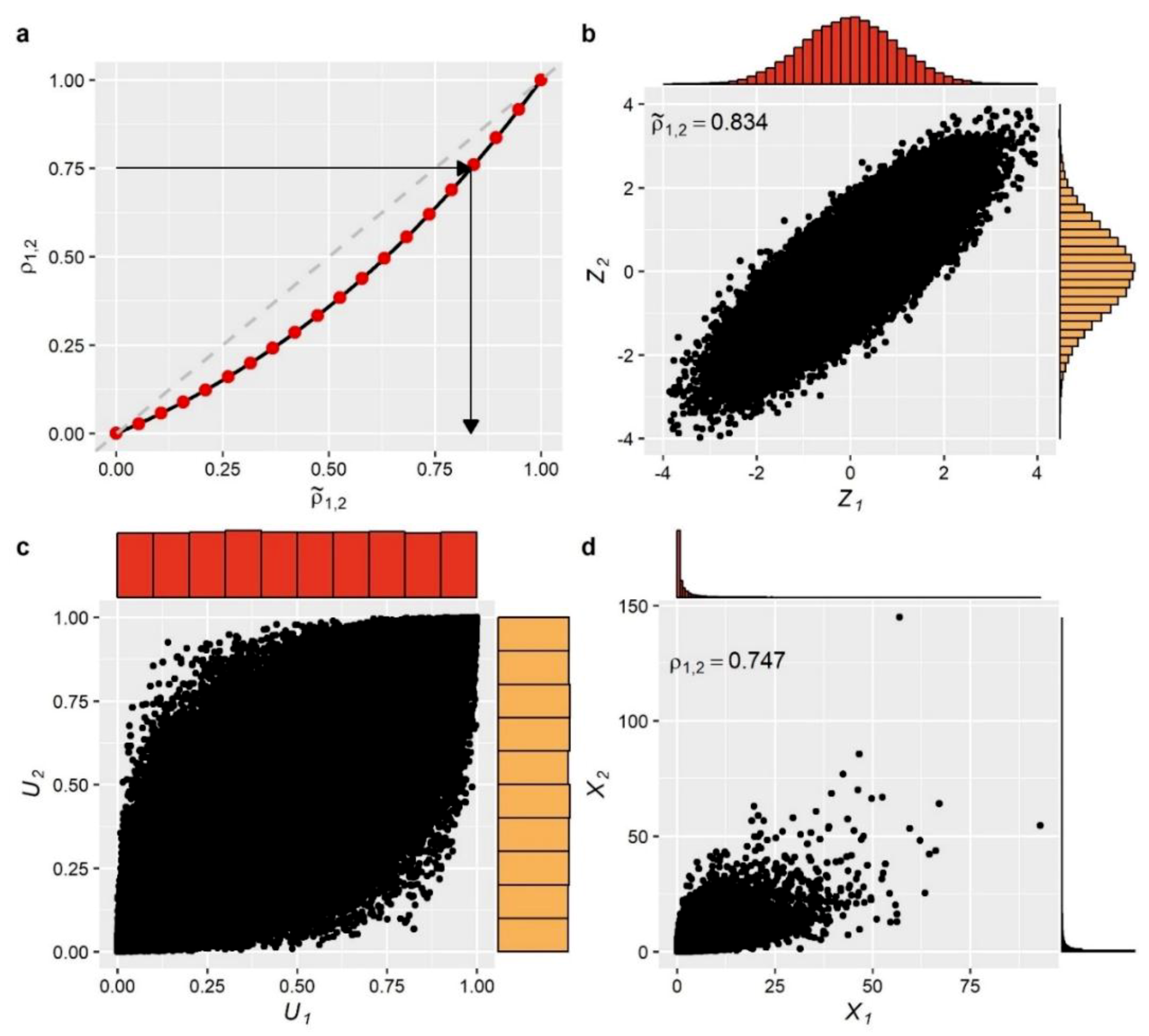
The established relationship between target and equivalent correlations is further illustrated in
Figure 2a. The equivalent correlation
of the Gaussian variables can be then obtained by solving the simple Equation (10) for the given target correlation. For this case, for
, we get
. Next, we generated 100,000 values from the bivariate standard normal distribution having the specified equivalent correlation. The scatter plot as well as the marginal distributions of these auxiliary variables are presented in
Figure 2b. These variables are first mapped to the uniform domain via the cdf of the standard normal distribution
, providing correlated values that have uniform marginal distributions (see
Figure 2c). The correlated uniformly distributed variables are then mapped to the actual domain (see
Figure 2d), according to Equation (1), to provide variables with the target marginal distributions and correlation. As explained above, the use of the ICDF of the target distribution (the Weibull in this example) as a mapping function ensures that the final variables will have the desired marginal properties, while the assignment of a technically inflated value to
allows to attain the target correlation
after the mapping operation.
2.6. Moving from Random Variables to Stochastic Processes
As already mentioned above, NDM can be also applied to generate synthetic time series with the desired marginal distributions and stochastic structure (in terms of autocorrelation and cross-correlation coefficients). In this case, a Gaussian process is employed to generate auxiliary time series which are then mapped via the ICDF of the target distributions to obtain the target process. Although Gaussian process can be regarded as an intermediate auxiliary step in the whole procedure, its role is crucial since its structure determines that of the target process, e.g., to simulate a stationary auto-correlated process then a stationary Gaussian process should be employed, while the generation of cyclostationary time series requires the use of a cyclostationary Gaussian model as auxiliary. Summarising, the choice of the auxiliary process that is going to be implemented in the NDM concept is a matter of modelling requirements and convenience.
As mentioned in
Section 2.1, different auxiliary models have been used in the existing Nataf-based schemes. In fact, as discussed in Tsoukalas et al. [
52], any linear stochastic model could be used to play this role. For instance, Papalexiou [
53] used the sum of independent autoregressive processes (e.g., see [
85,
86,
87]) to generate Gaussian time series.
In the present work, taking into account the peculiarities of residential water demand process at the timescales under study (i.e., hourly and sub-hourly scales) and without loss of generality, we employ stationary and cyclostationary autoregressive models to simulate the auxiliary Gaussian process. Prior describing these models, let us introduce some notations that allow the transition from random variables to processes.
Beginning from the stationary case, let
be a target process, where
is the time index, with target marginal distribution
and autocorrelation structure
, where
is the time lag. Furthermore, let
be the stationary Gaussian auxiliary process with zero mean and unit variance and autocorrelation structure
. In order to align the bivariate NDM, as presented in
Section 2.2 for the case of random variables, with stationary stochastic processes, we have to set throughout Equations (1)–(7),
and
for the target process, as well as
and
for the auxiliary, accordingly.
The most prominent linear stochastic model, used in a variety of applications and scientific fields, is the autoregressive model of order
(i.e., AR(
)). This can be attributed to its parsimony and simplicity as well as to its intuitive structure since the model implies that the present value of the process is obtained as the weighted sum of
past values and a random component. According to AR(
), a standard Gaussian process
, with specific autocorrelation structure
, is obtained by the following recursive formula:
where
are i.i.d variables (white noise) that follow the standard Normal distribution, i.e.,
, while
, with
, and
are model parameters. The parameters
are derived analytically on the basis of the Yule–Walker system, given the values of
up to lag
. This reads as:
where:
In order for an AR(
) process to be stationary, certain conditions for the parameters
should be fulfilled (e.g., see [
88]).
Parameter
essentially expresses the variance of the random component in Equation (11) and it can be estimated by:
In the AR() model, since are generated from the Normal distribution, the random process will be also Gaussian. Furthermore, this model ensures the preservation of a given autocorrelation structure up to lag , whereas for higher lags the model gives a gradually decay autocorrelation structure, i.e., at any lag the modelled autocorrelation is given by .
The stationary AR(
) model can be easily adjusted to account for cyclostationarity, i.e., in cases where the distribution and correlation structure of the process vary periodically from season-to-season. In this case, the model is termed as periodic autoregressive model of order
(i.e., PAR(
)), and further to the time index
, it is convenient to employ another index
that denotes the season (e.g.,
for processes exhibiting month-to-month variation or
for hour-to-hour variation). Subsequently, the cyclostationary process reads as
. Accordingly,
now represents the correlation between season
and
. Reasonably, model parameters will also depend on season
. Particularly, in the case of PAR(1) model, the model generating equation reads (the index
t is omitted for simplicity):
where
,
and
.
As presented in
Section 3, in the present work, AR(
) was used as an auxiliary model in the simulation of residential water demand processes at sub-hourly time scales (see
Section 3.1 and
Section 3.2), while to capture the hour-to-hour variation of hourly water demand (see
Section 3.3) we employ the PAR(1) model.
2.7. Modelling the Dependence Behaviour of Water Demand
Further to the marginal distributions, Nataf-based models aim to capture and reproduce the dependence behaviour of a process as expressed by its stochastic structure. As explained above, the use of Pearson’s correlation coefficient, as linear measure of dependence, arises naturally since linear stochastic models are employed to establish dependence in time. However, as it is known the estimation of empirical correlations, as well as of the other second-order statistics, subjects to important bias (e.g., [
89,
90]), especially in cases of small samples, large lags and intense (persistent) autocorrelation structures, i.e., large autocorrelation values that extend for large lags. This issue has been studied in the domain of hydrological variables (e.g., [
63,
91]), while Dimitriadis and Koutsoyiannis [
92] compare the suitability of other tools to identify the auto-dependence structure of a process. These sources of bias are also encountered in residential water demand processes since the available observed records are typically short, while their autocorrelation structure exhibits a more persistent behaviour as the time scale becomes finer. Due to this, a theoretical autocorrelation structure (ACS) is typically preferred over the direct use of the empirical sample estimates. Further to the above, the use of a suitable ACS is favored for a series of other reasons. Firstly, it ensures the stability of the linear stochastic models given that a properly defined ACS provides positive definite autocorrelation structures, which is a prerequisite so as the latter to be valid (see [
68] for more details). Furthermore, it can be regarded as a parsimonious procedure since the whole structure is described via a small set of parameters, enabling the extrapolation of correlation coefficients for lags as high as desired (1/3 of the sample size is the typically suggested as the maximum lag up to which empirical correlations can be properly estimated). Lastly, it enables the transferability of ACS parameters in cases where the sample size does not allow for a proper identification of the correlation structure and stable estimation of coefficients. The latter is of high importance in water demand modelling since observed records at fine time scales are typically limited both in terms of the number of meters and the length of records. In the present work, it is the first time that an ACS is employed to characterise the auto-dependence properties of residential water demand processes.
Various theoretical models to represent the correlation structure of stationary processes can be found in the literature (e.g., [
53,
86,
89,
90]). Here, we employ the Cauchy-type autocorrelation structure (CAS) proposed by Koutsoyiannis [
63] as a simple and parsimonious model, able to capture a wide range of short- and long-range dependence structures. The power-type CAS, for positive ACF, is given by:
where
and
are model parameters that control the form of the function and hence the degree of dependence. For
, CAS provides a short-range autocorrelation structure, i.e., an exponential structure that decays rapidly and diminishes after few time lags. On the contrary, for
, CAS resembles long-range autocorrelation structures, i.e., slowly decreasing structure that extends for large lags. For other values of parameters, the function provides the flexibility to represent autocorrelation structures between, or even outside of, the two cases explained above (see [
63] for further details).
The estimation of CAS parameters can be obtained by minimizing the error between the sample and theoretical correlation coefficients, on the basis of the least squares method. In the present study, our target was to achieve a good overall fit to a specific number of autocorrelations but with an extra care regarding the preservation of empirical lag-1, i.e., by setting a larger weight in the objective function for this quantity.
The above modelling strategy has been recently employed within NDM-based approaches for hydrological process modelling. In the NDM concept, Tsoukalas et al. [
52] used CAS model, while Papalexiou [
53] proposed a series of parametric ACS models exploiting their structural similarity with the form of common complementary cumulative distribution functions.
2.8. Summary of the Modelling Approach Step-by-Step
In the present section, we summarise the stochastic modelling framework for residential water demand processes via the following steps:
Select and fit the suitable marginal distributions (i.e., continuous, mixed; see
Section 2.4) and autocorrelation function (see
Section 2.7) that better capture the distributional properties and autocorrelation structures, respectively, of the observed time series.
Given the target autocorrelation structure
(derive either from a theoretical autocorrelation model or as it is estimated directly from the data), establish the correlation transformation function and estimate the equivalent correlation coefficient
up to the maximum specified lag
(see
Section 2.3).
Identify the suitable auxiliary Gaussian linear stochastic model (e.g., AR(
) and PAR(
); see
Section 2.6) and fit it on the basis of
.
Generate a realization of the auxiliary process at the Gaussian domain.
Use the ICDF of the fitted distribution to map the synthetic time series to the actual domain (i.e., Equation (1)) and obtain the final realization of the target process .
4. Summary and Conclusions
Due to the key role of water demand processes in the uncertainty-aware planning and management of urban water systems, the pursuit of adequately representing and simulating such processes has been a challenge that occupied many researchers over the years and resulted in the development of numerous simulation schemes. Depending on the time scale of analysis (which is typically a fine one), water demand processes exhibit a variety of marginal and dependence (expressed via auto-or cross-correlations) characteristics (e.g., non-Gaussianity, intermittency, auto-dependence) that should be reproduced by the stochastic model. However, already existing stochastic models provide a partial solution to the problem since they focus either on the marginal behavior of a process or on its dependence structure, and do not consider simultaneously both aspects.
Aiming to provide a remedy, and eventually a satisfactory modelling and simulation strategy for water demand processes, this work employs for the first time in the WDS modelling domain, the so-called Nataf-based stochastic models that entail the coupling of linear stochastic models with quantile mapping procedures. This type of models, recently employed to address challenging stochastic simulation problems for non-Gaussian hydrometeorological processes [
51,
52,
53], build upon the notion of Nataf’s joint distribution model [
47] which provides a sound theoretical background, as well as the necessary flexibility to account for a wide range of processes with arbitrary marginal distributions and correlation structures.
The generality, as well as the flexibility provided by the Nataf-based modelling strategy (detailed in
Section 2 and summarized in
Section 2.8) is stress-tested through three distinct simulation studies that are of particular interest for urban water systems (
Section 3). These concern the stochastic simulation of water demand processes at three characteristic time scales (i.e., 1-min, 15-min and 1-h), which arguably exhibit a variety of peculiarities, thus emphasizing different aspects of the method.
The main outcome from the simulation studies is that the employed modelling strategy is sufficient for the simulation of water demand process (stationary or cyclostationary) at any time scale (from 1 h down to 1 min), proving capable of reproducing simultaneously both the marginal and dependence properties of the processes without sacrificing neither precision nor parsimony. Particularly, it is highlighted that depending on the observed process characteristics, the method can be combined with a three-component mixed-distribution model (an additional contribution of this work) to provide an explicit representation of the entire target marginal distribution, accounting also for intermittency and tail behavior. Further to this, we move beyond the reproduction of empirical temporal correlations (typically involving few time lags) to a more complete and parsimonious description of the process’s temporal dependence properties through the use of theoretical correlation structures.
We argue that this work provides an interesting alternative to the prominent pulse-based methods (that mainly provide a moments-based representation of a process) for simulating water demand processes, introducing, for the first time within water demand process simulation, classic and easy to implement linear stochastic models. In our view, this approach, exploiting the flexibility (in terms of admissible distributions and correlations structures) of Nataf’s model, as well as knowledge derived from large scale studies (e.g., in the spirit of Kossieris and Makropoulos [
39]) which allow for a better understanding of the probabilistic laws and correlations that describe water demand, can greatly contribute to the widespread use of alternative stochastically generated water demand realizations, for a more uncertainty-aware design and management of urban water systems. Potential domains of future research could focus on the simulation of spatio-temporal water demand processes at node or household levels, thus accounting also for spatial dynamics. Furthermore, the proposed methodology could be also extended and studied in a disaggregation framework to allow the capturing of probabilistic and stochastic behaviour of water demand across multiple time scales, as well as for short-term and long-term forecasting.


