Abstract
A key issue in assessing the spatial distribution of flood risk is considering risk information derived from multiple flood sources (river flooding, drainage inundation, etc.) that may affect the risk assessment area. This study proposes a method for assessing spatial flood risk that includes flooding and inundation in small-basin areas through multivariate design rainfall. The concept of critical rainfall duration, determined by the time of concentration of flooding, is used to represent the characteristics of flooding from different sources. A copula method is adopted to capture the correlation of rainfall amounts in different critical rainfall durations to reflect the correlation of potential flooding from multiple flood sources. Rainfalls for different return periods are designed based on the copula multivariate analysis. Using the design rainfalls as input, flood risk is assessed following the rainfall–runoff–inundation–loss estimation procedure. A case study of the Otsu River Basin, Osaka Prefecture, Japan, was conducted to demonstrate the feasibility and advantages of this method. Compared to conventional rainfall design, this method considers the response characteristics of multiple flood sources, and solves the problem of flood risk assessment from multiple flood sources. It can be applied to generate a precise flood risk assessment to support integrated flood risk management.
1. Introduction
Spatial flood risk refers to the spatial distribution of flood risk across a risk assessment area. Since disaster risk is usually represented by a probability distribution of negative consequence [1], spatial flood risk refers to the spatial distribution of the probability distribution of loss. Therefore, for each unit of a flood risk assessment area, a risk curve that describes the exceedance probability distribution of loss should be estimated. Such spatial flood risk information is essential for various flood risk countermeasures, including risk controls: for example, improving safety and reliability of infrastructures [2] or risk financing: sharing risk using insurance or cat-bonds [3]. A flood risk assessment area can be affected by multiple flood sources: flooding from a main river, flooding from small rivers, inundation caused by heavy rainfall and drainage failure, even coastal flooding caused by storm surges, etc. A challenge in spatial flood risk assessment is to consider risk from such multiple flood sources.
From the perspective of “hazards of place” [4], flood risk from multiple sources can be viewed as a multi-hazard risk problem [5,6]. Although urban inundation, river flooding, coastal flooding, etc. are all grouped under flood hazard, their characteristics are not the same. For example, river flooding is related to dyke breaks, water overtopping the banks, and rainfall of the whole river basin. Assessing river flooding risk requires considering the problem in light of the spatial scale of the river basin and temporal scale of hours to days [7,8]. Because inundation is determined by drainage failure, urban topography, and intensive rainfall within the city, assessing urban inundation risk focuses on the spatial scale of a city and temporal scale of minutes to hours [9,10]. Such different considerations on temporal and spatial scale usually leads to the independent assessment of flood risk from multiple sources in practice. Flood risk needs to consider multiple flood sources, however, not just the sum of the risk examinations of each source. This is important because flood risks from multiple sources may be highly related; thus, they should be assessed in an integrated way.
The general framework for flood risk assessment, which includes the estimation of hazard, exposure, and vulnerability, has been well established by previous studies [11,12,13,14]. These studies have followed a procedure that includes the following: (1) the statistical analysis of rainfall or hydrological data, generating rainfall or flood events of a given frequency for simulating hazard information; (2) the estimation of exposure and vulnerability to evaluate the consequences of each rainfall or flood event; and (3) the integration of all scenarios to estimate the flood risk curve. Researchers continuously improve each step of the procedure by adopting new data from climate change projects and recent advances in technology [15], using high performance flood and inundation simulation models [16], focusing on the uncertainty of risk assessment [17], considering exposure and vulnerability change due to social development [18], and optimizing the risk assessment procedures for ungauged areas [19]. However, little attention has been paid to “multiple flood sources and their correlation” in the framework of flood risk assessment.
Therefore, to address the problem of flood risk from multiple sources, some specific steps are proposed. First, the flood risk assessment area’s response characteristics to hazards from different flood sources are identified. Then, their relationship is analyzed using multivariate statistical methods. Finally, this relationship is integrated into a simulation of multiple flood processes, which is followed by spatial flood risk assessment, since design rainfalls are often used for flood risk assessment in many areas. By applying this idea to design rainfall, we focus on the problem of how to integrate the assessment of flood risk from flooding and urban inundation, which has attracted much attention in Japan and other similar countries. Since many cities in Japan are located at the foot of mountains, flooding and inundation are closely related. Rainfall and runoff from mountain regions contribute to river flooding, while rainfall in the city contributes to urban inundation. However, both processes may affect urban areas independently or simultaneously. Capturing such joint effects is necessary for accurate spatial flood risk assessment.
When the basin area is small, meteorological conditions are usually similar within the basin and the spatial heterogeneity of rainfall can be ignored. Hence, spatially identically distributed design rainfall (hereafter, design rainfall) can be used for flood risk assessment. To assess spatial flood risk and include flooding and inundation, while considering design rainfall, the concept of critical rainfall duration determined by the time of concentration of flooding is introduced to represent the characteristics of flooding from different sources. Then, a copula method is adopted to capture the correlation between rainfall amounts for different critical rainfall durations and design rainfall with regard to different return periods. Taking design rainfall events as input, hazard information can be simulated by an integrated rainfall–runoff–inundation model. Flood risk in terms of economic loss is assessed by combining hazard, exposure, and vulnerability information.
2. Methodology
2.1. Design Rainfall and Flood Risk from Multiple Sources
Design rainfall is a synthetic rainfall amount and temporal pattern associated with a return period. Various methods for generating design rainfall for the purpose of river management or drainage planning can be found in the literature [20,21,22,23,24,25,26,27]. Design rainfall is also widely used for flood risk assessment, especially in areas without reliable hydrological time series. Design rainfall is naturally connected to flood risk assessment because it serves as an input for flood simulation. However, conventional rainfall design methods focus on analyzing rainfall data but rarely consider the requirements of flood risk assessment. For example, the procedure of conventional design rainfall-based flood and inundation risk assessment is shown in Figure 1. In this procedure, intensity-duration-frequency (IDF) analysis plays an important role. The rainfall used for flood risk assessment is designed from IDF curves. However, river flooding risk assessment may require consideration of longer duration design rainfall, whereas inundation risk assessment requires shorter duration design rainfall. Conventional IDF-based design rainfall may fail to catch such an important relationship and cause inaccuracy if river flooding and inundation risk are being assessed in combination. When assessing spatial flood risk, design rainfall should be able to directly or indirectly reveal the characteristics and relationship of flooding and inundation from multiple sources for the flood risk assessment area. It is necessary to rethink the conventional methods and consider the purpose of risk assessment and local peculiarities [28].
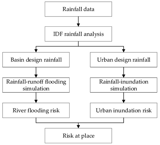
Figure 1.
Conventional design rainfall-based flood and inundation risk assessment procedure.
The response characteristics of a flood risk assessment area to flooding and inundation can be represented by the time of concentration, which is defined as the time required for rainwater to propagate from the top of a slope at the most remote portion of the basin to the outlet [29]. For small basins with a quick response time, it is reasonable to set the time of concentration as the critical rainfall duration, in which rainfall, including peak rainfall, will form the peak flood volume. As a flood’s concentration time may be different for different flood sources, the critical rainfall duration may also be different. The relationship between the response characteristics of flooding and inundation from different sources can therefore be treated as the correlation between rainfall amounts and different critical rainfall durations. Many empirical formulas have been proposed to estimate the time of concentration based on the natural characteristics of a basin (e.g., path length, basin slope, land use), including the Kraven’s formula, Izzard’s formula, Kodoya and Fukushima’s formula, Loukas and Quick’s formula, and Michailidi’s formula [21,30]. Predetermining the time of concentration from different flood sources and using them as critical rainfall durations to analyze rainfall data and generate rainfall events is likely to be an efficient way to assess spatial flood risk considering multiple flood sources.
Figure 2 illustrates the approach: on the left, the light-blue area is the risk assessment area; the pink areas are runoff areas. The design rainfall is shown above. It can be seen that a location (indicated by a star) in the risk assessment area will be affected by three flood sources: flooding from small river A, flooding from large river B, and inundation from the risk assessment area itself. For small basin A, the time of concentration is two hours, which means that a flood can reach the light-blue area in two hours from basin A. In basin A, a maximum rainfall within a two-hour period would most likely cause a flood in the risk assessment area (shown in the red box of the design rainfall). Likewise, for basin B, a maximum rainfall within a three-hour period would most likely cause a flood in the risk assessment area (shown in the green box of the design rainfall). For inundation in the risk assessment area caused directly by rainfall, the time of concentration would probably be very short. However, because usually only hourly data are available, the concentration time is defined as one hour. Hence, the probability distribution of a maximum one-hour rainfall reflects the maximum likelihood of inundation risk in the risk assessment area. The probability distribution of a maximum two-hour rainfall reflects the maximum likelihood of flooding risk from river A, and the probability distribution of a maximum three-hour rainfall reflects the maximum likelihood of flooding risk from river B. To evaluate the flood risk from both river A and river B, as well as the risk of inundation, the joint distribution of the maximum one-hour, two-hour, and three-hour rainfall events should be evaluated, and their correlation should be reflected in the rainfall design. The corresponding solution procedure based on multivariate rainfall design is presented in the right portion of Figure 2.
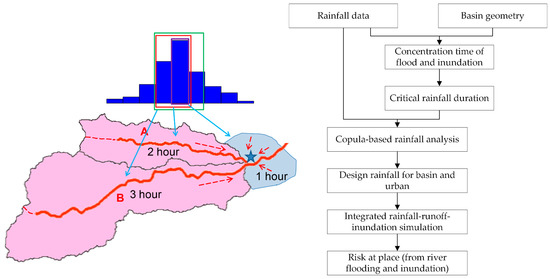
Figure 2.
Flood risk from flooding by two rivers and inundation, and the corresponding solution procedure.
2.2. Copula Method for Rainfall Design
Copulas are functions that join or “couple” multivariate distribution functions to one-dimensional marginal distribution functions [31]. For a bivariate case, the joint cumulative distribution function H(x,y) of any pair (x,y) of continuous random variables can be written as
where F(x) and G(y) are continuous marginal distributions, so that C:(0,1)2→(0,1) such that all is a copula [32]. This method separates joint distribution into a copula function and marginal distributions, and it has the advantage that the selection of an appropriate model for the dependence between varieties, represented by the copula, can then proceed independently of the choice of marginal distributions.
In this study, the copula method was adopted to analyze the correlations between and build joint distributions of rainfall amounts with critical rainfall durations for different flood sources, thus representing the correlations among them. Assuming there are n flooding sources that affect a risk assessment area, the critical rainfall duration for each flooding source is t1,t2…tn, and rt1, rt2… rtn are the rainfall amounts for critical rainfall durations. Then, a joint distribution can be derived as follows:
where F is the joint distribution, and F1, F2,… Fn are marginal distributions. Under the assumption of spatially identical rainfall, this joint distribution includes critical rainfall requirement information for multiple flooding sources. The steps for using the copula method are as follows:
First, the critical rainfall durations for each flooding source t1, t2…tn are identified. The empirical methods discussed in Section 2.1 can be used.
Second, the correlation of rainfall amounts with different critical rainfall durations is estimated—i.e., the copula function C is estimated.
Genest and Favre introduced some 20 types of copulas that may be suitable for hydrological studies, including Archimedean copulas, extreme value copulas, metaelliptical copulas, and other miscellaneous families of copulas [33]. For parameter estimation, a widely used method for estimating the copula parameter is a two-step parametric procedure, often referred to as the “inference from margins”, or IFM method [34]. This method first requires fitting a marginal distribution and then estimating the copula parameter via maximum likelihood estimation using data transferred from the marginal distribution. This method usually performs well, but association parameter estimates derived from IFM clearly depend on the choice of marginal distributions, and thus always risk being unduly affected if the models selected for the margins turn out to be inappropriate [35]. Since the dependence structure captured by a copula has nothing to do with the individual behavior of the variables, inferences about copula parameters rely only on the ranks of the observations. Instead of using a parametric method, rank-based nonparametric methods, such as the inversion of Kendall’s tau or Spearman’s rho, and semiparametric methods, such as Maximum Pseudo Likelihood, can be other possible choices.
There are two methods for constructing a high-dimensional copula: nested Archimedean construction (NAC) and pair copula construction (PCC). NAC is convenient for simple and nested structures; however, PCC is preferred as a more flexible method for multivariate copulas. PCC adopts a hierarchical idea and takes advantage of the density function. Its modeling scheme is based on a decomposition of multivariate density into d (d – 1)/2 bivariate copula densities, of which the first d – 1 is unconditional, and the rest are conditional [36]. There are two main types of PCC: canonical vines and D-vines [37]. D-vines are more frequently used; however, fitting a canonical vine is advantageous when a particular variable is known to be a key variable that governs interactions in the data set [38].
For copula selection, the characteristics of data and the size of data should be considered. The most intuitive approach would be through a graphical diagnostic: either directly compare a scatterplot of paired data with a copula-generated artificial data set, or compare the level curves of the empirical distribution with the level curves of the theoretical distribution [33]. In addition, information criteria, such as the Akaike information criterion (AIC) and Bayesian information criterion (BIC), frequently appear in some literature on copula application for the quantitative validation of the chosen copula [39]. Another means of quantitative validation is goodness of fit (GOF). Genest et al. reviewed goodness-of-fit tests for copulas and recommended some Cramer-von Mises statistics, including Sn, SnB, SnC, and SnK [40].
The third step is to fit the marginal rainfall distributions . Many studies have been conducted on fitting extreme rainfall distributions, and several types of distributions have been found that provide a good fit with rainfall data. However, no distribution can be universally fitted to all rainfall data due to the variable nature of rainfall, different purposes of studies, different locations, and so forth. For example, De Michele and Salvadori found generalized Pareto to be the best-fitted distribution [41], but Kao and Govindaraju found it to be the weakest [42]. Papalexiou and Koutsoyiannis used a generalized extreme value distribution to investigate the extreme daily rainfall all over the world and pointed out that the geographical location on the globe may affect the value of the shape parameter [43]. Therefore, the following strategy is normally used: several distributions, including Pearson distribution, generalized Pareto, generalized extreme value distribution, exponential distribution, gamma distribution, lognormal distribution, and Weibull distribution, are selected as candidates and tested for suitability based on a Kolmogorov–Smirnov test, as well as AIC.
The fourth step is to construct a joint distribution by combining step 2 and step 3. Once the marginal distributions and copula model are determined, the joint distribution can be constructed. Nelsen described joint distribution for a bivariable copula [31]. However, an explicit joint distribution for a high-dimensional copula is not always easy to obtain. Instead of using explicit joint distributions, the algorithms for sampling values from vine copulas proposed by Aas et al. can be used [37]. Note that the order of the steps is described in consideration of using the semiparametric method to estimate the copula function. If the parametric IFM method is used, the order of step 2 and step 3 is reversed.
Finally, rainfalls are designed based on the joint distribution according to the return periods. This step is empirical design work. A detailed description is provided in the case study section of this paper.
2.3. Spatial Flood Risk Assessment
Considering design rainfalls as input, the flood risk is assessed in terms of economic loss following the rainfall–runoff–inundation loss estimation procedure. A rainfall–runoff–inundation model combined with a geographic information system (GIS) is developed to support spatial flood risk assessment [44]. Design rainfalls are simulated to obtain the probability distribution of hazard information such as water depth, flow velocity, and so forth. Using exposure and vulnerability information, economic loss can be calculated. Economic loss encompasses property losses and business interruption losses [45]. Since hazard exposure and vulnerability information are both spatially distributed, economic losses can be spatially estimated.
In this study, design rainfalls are derived from the joint probability distribution. Therefore, for certain joint probabilities, various design rainfalls can be generated. Assuming is the exceedance probability of a rainfall event, and is the probability distribution of loss under the condition of rainfall occurrence, the exceedance probability of loss can be estimated using the following formula:
where represents the number of certain probabilities that are considered. Although the probability of hazard occurrence can be a continuous variable, given the cost of flooding and inundation simulation, usually only certain probabilities, such as 1/10, 1/20, 1/50, 1/100, and so forth, are considered. A sketch map is shown in Figure 3 to help understand the risk curve. The integrated blue areas conditioned on the probability of rainfall occurrence are the exceedance probabilities of loss x. The exceedance probability of includes the entire probability distribution of loss, when the probability of rainfall occurrence is low, and a part of the probability distribution of loss, when the probability of rainfall occurrence is relatively high. See references [3,46] for further discussion of the risk curve.
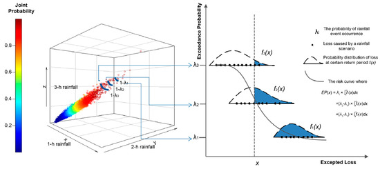
Figure 3.
Sketch map of the risk curve.
3. Case Study
3.1. Study Area
The study area is located in the southern part of Osaka Prefecture, Japan. The Otsu River, which originates in the Katsuragi Mountains and flows about 68 km westward to Osaka Bay, is a river within Osaka Prefecture that consists of five branches. The river basin extends from 34°20′ N to 34°30′ N and from 135°23′ E to 135°21′ E with an area of 102.2 km2, and it includes three cities. The average annual temperature in the study area is 16 °C, and the average annual rainfall is about 1200 mm. Rainfall data were derived from four rain gauging stations with 49 years of hourly rainfall records.
Historical records show that the study area has been prone to flood-related disasters. From 1950 to 2011, 14 flooding events were recorded. Local inundation and river flooding are the main causes of flood-related disasters. In particular, the downstream portion of the basin, which is flat and characterized by the confluence of three rivers, has a high probability of flooding from these rivers and from local inundation. In addition, population and properties are concentrated in the downstream portion of the basin. Accordingly, this area should first be considered as a risk assessment area (RAA). For the risk assessment area, flood sources include river flooding from the Ushitaki River, which is controlled by runoff in the upper part of the Ushitaki sub-basin (SB1); river flooding from the Matsuo River, which is controlled by runoff in the upper part of the Matsuo sub-basin (SB2); river flooding from the Makio River, which is controlled by runoff in the upper part of the Makio sub-basin (SB3); and local inundation from urban drainage or slope flow, which is controlled by runoff in the flood risk assessment area. A map of the Otsu River Basin is shown in Figure 4.
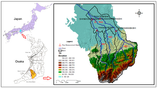
Figure 4.
Map of the study area.
3.2. Rainfall Analysis and Rainfall Design
3.2.1. Identification of Critical Rainfall Durations and Rainfall Data Pre-Processing
According to the empirical Kraven formula [9], the flood concentration time for SB1 is 2 h, 1.6 h for SB2, and 2.7 h for SB3. Since there is no large reservoir or dam in the runoff areas, the flood concentration time suggests that a 2 h maximum rainfall amount in SB1 and SB2, and a 3 h maximum rainfall amount in SB3 will produce a flood peak in the risk assessment area. For the flood concentration time in the risk assessment area itself, a 1 h rainfall amount is considered critical. Thus, the analysis of the joint probability of flooding from multiple sources becomes an analysis of the joint probability of 1 h, 2 h, and 3 h rainfall amounts under the assumption of spatially identical rainfall. Before the analysis, rainfall data were pre-processed, which included obtaining the basin average rainfall from four rain gauging station data by the Thiessen polygon method and dividing the rainfall time series into rainfall events using the interval time method [20,47,48].
3.2.2. Estimating the Correlation of Rainfall Amounts with Different Critical Rainfall Durations
Although all rainfall data could be used to evaluate the dependence structure, flood risk analysis is more concerned with extreme rainfall events. Therefore, annual maximum rainfall events corresponding to 1 h, 2 h, and 3 h durations were selected. Data triplets were selected to analyze the correlations of the maximum 1 h, 2 h, and 3 h rainfall amounts in extreme rainfall events. For each year, using the annual maximum 1 h rainfall amount as a criterion, an extreme event is selected. Then, one triplet of (1 h, 2 h, 3 h) rainfall amount data is obtained. The same is done using the annual maximum 2 h or maximum 3 h rainfall amount as a criterion. Since we have 49 years’ worth of records, we have 49 × 3 = 147 triplets. However, many of the triplets overlap because annual maximum 1 h, 2 h, and 3 h rainfall amounts may occur during the same rainfall event, or two of them may occur during the same rainfall event. Removing repeated triplets resulted in 68 data triplets (1 h, 2 h, 3 h rainfall amounts), which were adopted for the trivariate copula analysis.
In our study, peak rainfall is treated as the key variable, and the relationship between 1 h rainfall amount and 2 h rainfall amount, or the relationship between 1 h rainfall amount and 3 h rainfall amount, is relatively more important than the relationship between 2 h rainfall amount and 3 h rainfall amount. Therefore, a three-dimensional canonical vine was constructed. To reduce uncertainties from the choice of marginal distributions, the maximum pseudo-likelihood method was used for parameter estimation.
Among the roughly 20 types of copulas mentioned in Section 2.2, AIC shows that a Gumbel survival copula with a parameter of 3.357, a Gaussian copula with a parameter of 0.804, and a BB7 copula with parameters of 2.923 and 3.451 can properly fit the 1 h/2 h rainfall correlation, the 1 h/3 h rainfall correlation, and the conditional 2 h/3 h rainfall correlation, respectively. Figure 5 shows 3-D scatter points of pseudo data and fitted copula densities for 1 h/2 h, 1 h/3 h, and conditional 2 h/3 h rainfall amounts, from which the correlation of rainfall amounts of different durations can be illustrated.
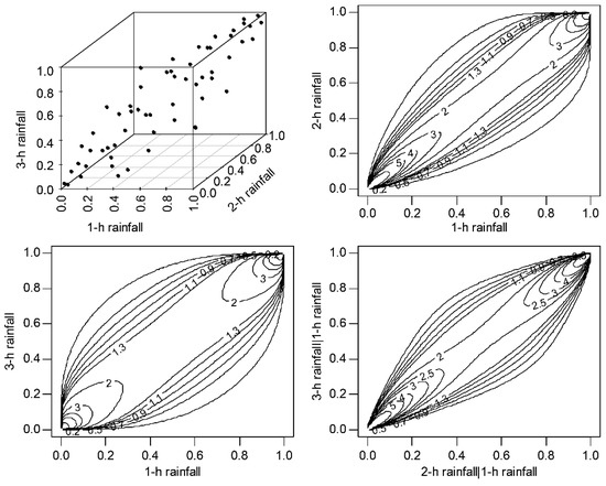
Figure 5.
3-D scatter plot of pseudo data and fitted copula densities for 1-h/2-h, 1-h/3-h, and conditional 2-h/3-h rainfall amounts.
3.2.3. Fitting of Marginal Distributions
A major advantage of constructing copula-based joint distributions is that the copula structure and marginal distribution can be estimated independently. The 68 data triplets are used to estimate the copula structure. However, according to block extreme value theory, for each year, only one value for each 1 h, 2 h, and 3 h rainfall amount can be used. Therefore, three sets of 49 data points are used to estimate the marginal distribution. The AIC and KS tests indicate that among the set of candidate distributions mentioned in Section 2.2, for annual maximum 1 h rainfall, the best-fitting distribution is a lognormal distribution with parameter (3.098, 0.359); for annual maximum 2 h rainfall, the best-fitting distribution is Pearson 3 with parameter (1.76, 16.259, 10.725); and for annual maximum 3 h rainfall, the best-fitting distribution is lognormal with parameter (3.672, 0.369), as shown in Figure 6.

Figure 6.
Marginal distributions of annual maximum 1-h, 2-h, and 3-h rainfall amounts.
3.2.4. Construction of Joint Distributions and Generation of Correlated Critical Rainfall
Taking advantage of algorithms proposed by Aas et al. [37], random copula values can be generated. Then, a random value of rainfall amount with critical durations can be obtained as the inverse of the marginal distributions. Figure 7 shows 10,000 random values generated by copula functions together with observed real rainfall data. From this figure, it can be seen that the correlation of real rainfall data is captured by the copula model. Therefore, it is reasonable to use the simulated random values for flood risk assessment.
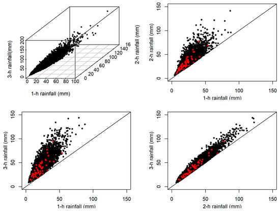
Figure 7.
Plots of 10,000 random rainfall values generated by the copula model. Black dots are random values; red dots represent observed real rainfall data.
3.2.5. Design and Generation of Rainfall Based on Joint Distribution
Assuming a peak appears at the center of each rainfall event, the amount of 1 h, 2 h, and 3 h rainfall can be distributed in the following way: Let Tp represent the time of peak rainfall, rtp represent the amount of peak rainfall, and r1h, r2h, r3h represent the 1 h, 2 h, and 3 h rainfall amounts simulated from the joint distribution of rainfall events, respectively. The rainfall amount for the critical duration of three hours can be determined as follows: rtp = r1h; rtp-1 = r2h-r1h; rtp+1 = r3h-r2h. Since the generated rainfall data contain not only information about 1 h, 2 h, and 3 h rainfall amounts, but also information about the joint probability of these events, the design rainfall event will share the same probability. In addition to the critical rainfall durations, the remaining duration of a rainfall event will also affect runoff but contribute less to the flood peak. Therefore, the remaining duration can simply be added using the statistical average of historical rainfall events. Using this strategy, rainfall was designed for the case study area. Because a joint probability function was adopted, more than one rainfall value can be expected for a certain return period. In Figure 8, five rainfall events with 50-year and 100-year return periods are shown. The generated rainfall can be interpreted as the design rainfall, which includes contributions from multiple flood sources such as, in our study, river flooding from the Ushitaki, Matsuo, and Makio Rivers, and local inundation from urban drainage. It is obvious that even for the same return period, variations in generated rainfall reflect different combinations of floods from different sources.
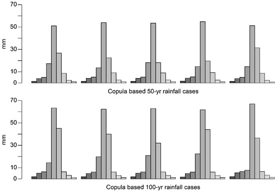
Figure 8.
Five rainfall cases for 50-year and 100-year return periods from copula-based rainfall analysis. The y-axis is rainfall amount, the x-axis is rainfall duration; 9-h rainfall events are designed.
3.3. Spatial Flood Risk Assessment
Using the design rainfall from the previous section as input, flood scenarios under different rainfall situations can be simulated. Figure 9 presents two examples of flood simulations under different rainfall scenarios but with the same return period. Based on this flood simulation, the spatial distribution of hazards can be understood. It is interesting to note that due to the joint probability analysis of rainfall, different rainfall scenarios can be generated, even under one joint probability; thus, inundation can be different, even for the same return period.
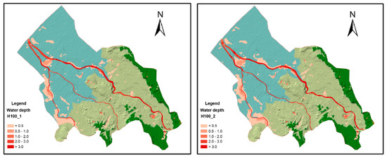
Figure 9.
Example of flood simulations (maximum inundation depth) under different rainfall scenarios using a 100-year return period.
To evaluate property loss caused by floods, exposure data such as population density, enterprises, industrial types, and number of employees should be considered. This information can be obtained and processed from the census and economic census data of Japan. Fragility curve information, which describes the relationship between water depth and loss ratio, can be found in [45,49].
Loss can be calculated by combining hazard, exposure, and vulnerability. A risk curve can be estimated after calculating all rainfall events using Equation (3). Figure 10 shows an example of a risk curve for a single mesh cell. For each return period, expressed here as exceedance probability, several rainfall events are generated. As stated above, the rainfall events are simulated from the joint distribution of rainfall amounts of different critical durations, which represent the influence of different flooding sources on the risk assessment area. Therefore, the distribution of loss at a certain return period reveals the uncertainty of the combination of floods from different flooding sources. It is obvious that as many rainfall events as possible should be included to produce a better fit of the loss distribution for each return period. However, given the cost of flood simulation, only a limited number of rainfall events are chosen. This can be improved in future studies. The risk curve describes the exceedance probability distribution of loss. For example, in Figure 10, the exceedance probability of economic loss of 140,000 Japanese yen is about 0.02, which means, considering all the floods that may happen in this area, the probability of economic loss beyond 140,000 is about 0.02.
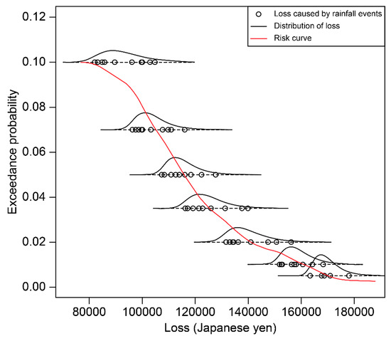
Figure 10.
Risk curve in terms of economic loss. (The exchange rate between U.S. dollar and Japanese yen is about 1:111.).
Figure 11 shows the spatial distribution of flood risk in terms of expected loss, which is an integration of the risk curve. From the figure, it can be seen that there are four locations at risk in the study area: the area along the middle of Ushitaki River, the area between Matsuo downstream and Makio downstream, and the area to the right of Makio downstream and the upper part of Makio River. It seems that the expected loss in each mesh is not very large. On one hand, this result is due to the small size of the mesh, which includes limited exposures. On the other hand, as Haimes pointed out, expected loss may make risk look moderate [50]. However, the risk curve at each mesh provides complete flood risk information. It is interesting to note that both the values and the shapes of the risk curves can be very different from mesh to mesh, which reveals the local flood risk characteristics. For example, the risk curve of a mesh between Matsuo downstream and Makio downstream (as shown in the top left of Figure 11) shows a gentle slope at the tail. Compared with the risk curve of a mesh along the middle of Ushitaki River (as shown in the bottom left of Figure 11), this result indicates that the former area is relatively more sensitive to the hazard return period. If the occurrence probability changes from once in 50 years to once in 200 years, the economic loss in the former area increases more than in the latter area. In other words, considering the economic reasonability, to prevent flood risk, countermeasures in the former area should take into account extreme events that occur once in 100 years or more; however, in the latter area, it is sufficient for countermeasures to take into account events that occur once in 50 years.
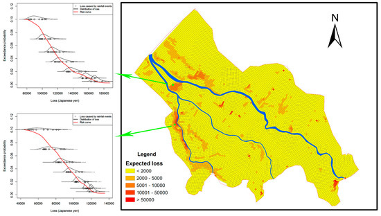
Figure 11.
Spatial flood risk map for expected economic loss and three examples for risk curves at different locations. (The exchange rate between U.S. dollar and Japanese yen is about 1:111).
4. Discussion
The proposed methodology for spatial flood risk assessment in small-basin areas considering both inundation and flooding is based on a reinterpretation of design rainfall. The design rainfall in this study is not only a result of statistical analysis of rainfall data, but also gives significant consideration to flood simulation input. Thus, it accounts for risk characteristics of different flood sources. Therefore, in the process of rainfall statistical analysis and rainfall design, emphasis is placed on pre-estimation of response characteristics of a flood risk assessment area to different flood risk sources and reflecting these characteristics into rainfall design.
This study began with the problem of how to assess flood risk from multiple flood sources. However, with the assumption of spatially identical rainfall, it focused on the problem of the temporal correlation of design rainfall. Compared to design rainfall methods based on conventional intensity-duration-frequency (IDF) curves (e.g., the Chicago method), our approach has two advantages for solving the problem of flood risk assessment from multiple flood sources: (1) Critical rainfall durations are determined by the time of concentration of flooding from different flood sources that connect flood risk assessment with design rainfall. (2) Copula-based rainfall analysis considers the joint distribution of rainfall amounts with different critical durations, which enables the generation of different types of rainfalls rather than a deterministic type of rainfall for a certain return period. In addition, since copula-based design rainfall uses joint probability and IDF-curve-based design rainfall uses only marginal probability, according to the copula’s Frechet–Hoeffding bounds [30], given a return period, copula-based design rainfall will always be larger than IDF-curve-based design rainfall, as illustrated in Figure 12. With regard to this study, this phenomenon can also be interpreted such that flooding from multiple sources will always be more dangerous than flooding from only a single source. Hence, flood risk will be underestimated when conventional IDF-curve-based design rainfall is applied to consider flooding from multiple flood sources.

Figure 12.
Comparison of 1-h, 2-h, and 3-h rainfall calculated using the copula-based design rainfalls and the IDF-curve-based ones for 1/50 and 1/20 events.
The proposed methodology is suitable for small-basin areas, where spatially identical rainfall can be used for estimating both river flooding and urban inundation. For larger study areas, river flooding and urban inundation may be controlled by different rainfalls. In these situations, more complex spatiotemporal correlations of rainfall should be considered. Besides design rainfall, stochastic-based rainfall generators which preserve the auto- and cross-dependence structures across scales provide alternative approaches to consider this problem. However, the precision of generated rainfall time series data is sometimes not satisfactory. Nonetheless, these approaches are being continuously developed [51,52] and could be better in the future. In recent studies, long-term climate ensemble forecasting data simulated by global circulation model (GCM) or regional climate model (RCM) are used for flood risk assessments [15,46]. It is a possible solution for solving problems regarding flood risk from multiple sources. However, the high cost and uncertainties of ensemble forecasting prevent the widespread use of this method in flood risk assessment practice. Methodologies based on traditional rainfall analysis and rainfall design are still worthy of further study.
5. Conclusions
This study has proposed a new methodology for spatial flood risk assessment in small-basin areas considering both inundation and flooding. A case study, conducted in the Otsu River Basin, Osaka prefecture, Japan, demonstrates this methodology. From this study, the following conclusions can be drawn.
(1). Considering risk information derived from multiple flood sources that may affect the risk assessment area is an important issue in assessing the spatial flood risk. Design rainfalls are usually used for flood risk assessment: however, the conventional method of design rainfall may lead to an underestimation of flood risk.
(2). This study illustrates that the copula method is suitable for constructing a joint probability distribution for rainfall design. Under the assumption of spatially identical rainfall, copula-based design rainfall provides a possible solution for small basin areas to consider flood risk from both inundation and river flooding. In addition, the requirement for an integrated rainfall–runoff–inundation simulation is also emphasized.
(3). Many previous studies concerned with “hazard of place” use a weighted index to integrate multi-hazards [4,5], which is reasonable if the relation between multi-hazards is weak. However, some closely related hazards, such as urban inundation, river flooding, and coastal storm surge inundation, should be integrated in a more realistic way. In this paper, we trace urban inundation and river flooding to rainfall, reflect their relation through design rainfall and integrated flood simulation, and, finally, adopt the risk curve at mesh to represent the total flood risk from multiple sources.
(4). Risk curve at meshes provides complete spatial flood risk information [46]. Using expected value, conditional expected value, or value of certain return periods calculated from the risk curves as indicators, risk maps can be made. In the case study, the main areas at risk are identified. The risk curve at meshes can facilitate integrated flood risk countermeasures. For example, through the spatially distributed risk curve, policy makers can determine in which place they should adopt a 1/100 years mitigation measure and in which place a 1/50 years mitigation measure is economically reasonable. Also, the spatially distributed risk curves provide basic information for risk transfer and risk sharing between areas, and agreements to this end can only be researched in areas that accurately understand their own and others’ risk.
Further study in this area will be focused on two aspects: First, the proposed methodology of design rainfall is suitable only for flood risk assessment in small river basins because of the assumption of spatially identical rainfall. Future research could be conducted to extend analysis to large river basins by considering more complex spatiotemporal correlations. Second, this paper provides a new way to view the problem of “hazard of place”. Additional hazards, besides river flooding and inundation, can be included as technology improves and the estimation of high dimensional correlations and the development of simultaneous multi-hazards simulation models becomes more feasible.
Author Contributions
Conceptualization, H.T. and X.J.; methodology, H.T. and X.J.; software, X.J.; formal analysis, L.Y. and X.J.; investigation, X.J.; resources, L.Y.; data curation, H.T.; writing—original draft preparation, X.J. and L.Y.; writing—review and editing, X.J. and L.Y.; visualization, X.J.; supervision, H.T.; project administration, H.T.; funding acquisition, L.Y. and H.T.”
Funding
This study was supported by the National Natural Science Foundation of China (Grant No. 41807504) and Fundamental Research Funds for Central Universities (WUT: 2019VI032,2019IVB002), China. This work was also supported under the framework of the Integrated Hazards Projections in the Integrated Research Program for Advancing Climate Models (TOUGOU Program) supported by the Ministry of Education, Culture, Sports, Science, and Technology of Japan (MEXT).
Conflicts of Interest
The authors declare no conflict of interest.
References
- Haimes, Y.Y. Systems-Based Guiding Principles for Risk Modeling, Planning, Assessment, Management, and Communication: Systems-Based Guiding Principles. Risk Anal. 2012, 32, 1451–1467. [Google Scholar] [CrossRef]
- Pietrucha-Urbanik, K.; Tchórzewska-Cieślak, B. Approaches to Failure Risk Analysis of the Water Distribution Network with Regard to the Safety of Consumers. Water 2018, 10, 1679. [Google Scholar] [CrossRef]
- Tatano, H.; Takagi, A. Economic Analysis of Disaster Prevention: Policy and Evaluation of Risk Management; Keisoshobo Press: Tokyo, Japan, 2005. (In Japanese) [Google Scholar]
- Greiving, S. Integrated Risk Assessment of Multi-Hazards: A New Methodology. Special Paper-Geological Survey of Finland. 2006. Available online: http://citeseerx.ist.psu.edu/viewdoc/download?doi=10.1.1.668.5877&rep=rep1&type=pdf (accessed on 10 May 2019).
- Kappes, M.S.; Keiler, M.; Elverfeldt, K.; Glade, T.; Von Elverfeldt, K. Challenges of analyzing multi-hazard risk: A review. Nat. Hazards 2012, 64, 1925–1958. [Google Scholar] [CrossRef]
- Schmidt, J.; Matcham, I.; Reese, S.; King, A.; Bell, R.; Henderson, R.; Smart, G.; Cousins, J.; Smith, W.; Heron, D. Quantitative multi-risk analysis for natural hazards: a framework for multi-risk modelling. Nat. Hazards 2011, 58, 1169–1192. [Google Scholar] [CrossRef]
- Sun, P.; Wen, Q.; Zhang, Q.; Singh, V.P.; Sun, Y.; Li, J. Nonstationarity-based evaluation of flood frequency and flood risk in the Huai River basin, China. J. Hydrol. 2018, 567, 393–404. [Google Scholar] [CrossRef]
- Tanaka, T.; Tachikawa, Y.; Ichikawa, Y.; Yorozu, K. Impact assessment of upstream flooding on extreme flood frequency analysis by incorporating a flood-inundation model for flood risk assessment. J. Hydrol. 2017, 554, 370–382. [Google Scholar] [CrossRef]
- Chen, W.; Huang, G.; Zhang, H.; Wang, W. Urban inundation response to rainstorm patterns with a coupled hydrodynamic model: A case study in Haidian Island, China. J. Hydrol. 2018, 564, 1022–1035. [Google Scholar] [CrossRef]
- Yang, T.-H.; Hwang, G.-D.; Tsai, C.-C.; Ho, J.-Y. Using rainfall thresholds and ensemble precipitation forecasts to issue and improve urban inundation alerts. Hydrol. Earth Sci. Discuss. 2016, 20, 1–24. [Google Scholar]
- Plate, E.J. Flood risk and flood management. J. Hydrol. 2002, 267, 2–11. [Google Scholar] [CrossRef]
- Van Dyck, J.; Willems, P. Probabilistic flood risk assessment over large geographical regions: Probabilistic flood risk. Water Resour. Res. 2013, 49, 3330–3344. [Google Scholar] [CrossRef][Green Version]
- Taki, K.; Matsuda, T.; Ukai, E. Method for evaluating flood disaster reduction measures in alluvial plains. J. Flood Risk Manag. 2013, 6, 210–218. [Google Scholar] [CrossRef]
- Dottori, F.; Salamon, P.; Bianchi, A.; Alfieri, L.; Hirpa, F.A.; Feyen, L. Development and evaluation of a framework for global flood hazard mapping. Adv. Water Resour. 2016, 94, 87–102. [Google Scholar] [CrossRef]
- Alfieri, L.; Feyen, L.; Dottori, F.; Bianchi, A. Ensemble flood risk assessment in Europe under high end climate scenarios. Environ. Chang. 2015, 35, 199–212. [Google Scholar] [CrossRef]
- Liang, Q.; Xia, X.; Hou, J. Efficient urban flood simulation using a GPU-accelerated SPH model. Environ. Earth Sci. 2015, 74, 7285–7294. [Google Scholar] [CrossRef]
- Apel, H.; Thieken, A.H.; Merz, B.; Bloschl, G. Flood risk assessment and associated uncertainty. Hazards Earth Sci. 2004, 4, 295–308. [Google Scholar] [CrossRef]
- Grahn, T.; Nyberg, L. Assessment of pluvial flood exposure and vulnerability of residential areas. Int. J. Disaster Risk Reduct. 2017, 21, 367–375. [Google Scholar] [CrossRef]
- Papaïoannou, G.; Efstratiadis, A.; Vasiliades, L.; Loukas, A.; Papalexiou, S.M.; Koukouvinos, A.; Tsoukalas, I.; Kossieris, P. An Operational Method for Flood Directive Implementation in Ungauged Urban Areas. Hydrology 2018, 5. [Google Scholar] [CrossRef]
- Huff, F.A. Time distribution of rainfall in heavy storms. Water Resour. Res. 1967, 3, 1007–1019. [Google Scholar] [CrossRef]
- Japan Society of Civil Engineers. The Collection of Hydraulic Formulae; Maruzen Publishing Co. Ltd.: Tokyo, Japan, 1999. (in Japanese) [Google Scholar]
- Keifer, C.J.; Chu, H.H. Synthetic storm pattern for drainage design. J. Hydraul. Division 1957, 83, 1–25. [Google Scholar]
- US Army Corps of Engineers. Hydrologic Modeling System HEC-HMS (Technical Reference Manual); United States Army Corps of Engineers: Davis, California, 2000.
- US Department of Agriculture. Urban Hydrology for Small Watersheds (Technical Release 55); US Department of Agriculture: Washington, DC, USA, 1986.
- Villani, P.; Veneziano, D. Best linear unbiased design hyetograph. Water Resour. Res. 1999, 35, 2725–2738. [Google Scholar]
- Watt, W.E.; Chow, K.C.A.; Hogg, W.D.; Lathem, K.W. A 1-h urban design storm for Canada. Can. J. Civ. Eng. 1986, 13, 293–300. [Google Scholar] [CrossRef]
- Yen, B.C.; Chow, V.T. Design hyetographs for small drainage structures. J. Hydraul. Division 1980, 106, 1055–1076. [Google Scholar]
- Efstratiadis, A.; Koussis, A.D.; Koutsoyiannis, D.; Mamassis, N. Flood design recipes vs. reality: Can predictions for ungauged basins be trusted? Hazards Earth Sci. 2014, 14, 1417–1428. [Google Scholar] [CrossRef]
- Kadoya, M.; Fukushima, A. Concentration Time of Flood in Small or Medium River Basin; Annual Report Number 19; Disaster Prevention Research Institute: Kyoto, Japan, 1976; pp. 143–152. (in Japanese) [Google Scholar]
- Michailidi, E.M.; Antoniadi, S.; Koukouvinos, A.; Bacchi, B.; Efstratiadis, A. Timing the time of concentration: shedding light on a paradox. Hydrol. Sci. J. 2018, 1–20. [Google Scholar] [CrossRef]
- Nelsen, R. An Introduction to Copulas, 2nd ed.; Springer: New York, NY, USA, 2006. [Google Scholar]
- Sklar, A. Fonctions de repartition an dimensions et leurs marges. Publications de l’Institut Statistique de l’Université de Paris 1959, 8, 229–231. (in French). [Google Scholar]
- Genest, C.; Favre, A.-C. Everything You Always Wanted to Know about Copula Modeling but Were Afraid to Ask. J. Hydrol. Eng. 2007, 12, 347–368. [Google Scholar] [CrossRef]
- Joe, H. Multivariate Models and Dependence Concepts; Chapman & Hall: London, UK, 1997. [Google Scholar]
- Choroś, B.; Ibragimov, R.; Permiakova, E. Copula Estimation. In Copula Theory and Its Applications. Lecture Notes in Statistics (77–91); Springer: Heidelberg, Berlin, 2010. [Google Scholar]
- Aas, K.; Berg, D. Models for construction of multivariate dependence—A comparison study. Eur. J. Finance 2009, 15, 639–659. [Google Scholar] [CrossRef]
- Kurowicka, D.; Cooke, R. Sampling algorithms for generating joint uniform distributions using the vine-copula method. Comput. Stat. Data Anal. 2007, 51, 2889–2906. [Google Scholar] [CrossRef]
- Aas, K.; Czado, C.; Frigessi, A.; Bakken, H. Pair-copula constructions of multiple dependence. Insur. Math. Econ. 2009, 44, 182–198. [Google Scholar] [CrossRef]
- Karmakar, S.; Simonovic, S. Bivariate flood frequency analysis. Part 2: A copula-based approach with mixed marginal distributions. J. Flood Risk Manag. 2009, 2, 32–44. [Google Scholar] [CrossRef]
- Genest, C.; Remillard, B.; Beaudoin, D. Goodness-of-fit tests for copulas: A review and a power study. Insur. Math. Econ. 2009, 44, 199–213. [Google Scholar] [CrossRef]
- De Michele, C.; Salvadori, G. A Generalized Pareto intensity-duration model of storm rainfall exploiting 2-Copulas. J. Geophys. Res. Biogeosciences 2003, 108, 1–11. [Google Scholar] [CrossRef]
- Kao, S.-C.; Govindaraju, R.S. A bivariate frequency analysis of extreme rainfall with implications for design. J. Geophys. Res. Biogeosciences 2007, 112, 1–15. [Google Scholar] [CrossRef]
- Papalexiou, S.M.; Koutsoyiannis, D. Battle of extreme value distributions: A global survey on extreme daily rainfall. Water Resour. Res. 2013, 49, 187–201. [Google Scholar] [CrossRef]
- Jiang, X. A Methodology for Assessment of Spatial Distribution of Flood Risk. Doctoral Dissertation, Kyoto University, Kyoto, Japan, 2014. [Google Scholar]
- Jiang, X.; Mori, N.; Tatano, H. Estimation of property loss and business interruption loss caused by storm surge inundation due to climate change: a case of Typhoon Vera revisit. Natural Hazard 2016, 84, 35–49. [Google Scholar] [CrossRef]
- Jiang, X.; Mori, N.; Tatano, H.; Yang, L. Simulation-Based Exceedance Probability Curves to Assess the Economic Impact of Storm Surge Inundations due to Climate Change: A Case Study in Ise Bay, Japan. Sustainability 2019, 11, 1090. [Google Scholar] [CrossRef]
- Dairaku, K.; Emori, S.; Oki, T. Rainfall Amount, Intensity, Duration, and Frequency Relationships in the Mae Chaem Watershed in Southeast Asia. J. Hydrometeorol. 2004, 5, 458–470. [Google Scholar] [CrossRef]
- Jones, P.D.; Hulme, M. Calculating Regional Climatic Time Series for Temperature and Precipitation: Methods and Illustrations. Int. J. Clim. 1996, 16, 361–377. [Google Scholar] [CrossRef]
- Yang, L.; Kajitani, Y.; Tatano, H. A methodology for estimating business interruption loss caused by flood disasters: Insights from business surveys after Tokai Heavy Rain in Japan. Natural Hazards 2016, 84, 411–430. [Google Scholar] [CrossRef]
- Haimes, Y.Y. Risk modeling, Assessment, and Management; John Wiley & Sons: Hoboken, NJ, USA, 2015. [Google Scholar]
- Kossieris, P.; Makropoulos, C.; Onof, C.; Koutsoyiannis, D. A rainfall disaggregation scheme for sub-hourly time scales: Coupling a Bartlett-Lewis based model with adjusting procedures. J. Hydrol. 2018, 556, 980–992. [Google Scholar] [CrossRef]
- Park, J.; Onof, C.; Kim, D. A hybrid stochastic rainfall model that reproduces some important rainfall characteristics at hourly to yearly timescales. Hydrol. Earth Sci. 2019, 23, 989–1014. [Google Scholar] [CrossRef]
© 2019 by the authors. Licensee MDPI, Basel, Switzerland. This article is an open access article distributed under the terms and conditions of the Creative Commons Attribution (CC BY) license (http://creativecommons.org/licenses/by/4.0/).