1. Introduction
As an important hydraulic engineering measure for human utilization and management of water resources, reservoirs have effectively solved the contradiction between the allocation of water resources and the demand of human economy and society development. As a powerful tool for the guidance of the reservoir operation, the reservoir operating plan is not only the decision-making reference factor of water conservancy project in the period of planning and design, but also the key to the impact of the comprehensive benefits of the reservoir during the operation and management period. Therefore, a reasonable and effective reservoir operating plan is essential for the implementation of reservoir function and the coordination of contradiction among multiple functional goals, such as flood control, water supply, power generation, shipping, and ecological purposes [
1,
2,
3].
At present, reservoir operation is mainly based on the operating diagram or the operating function (such as linear function, neural network, fuzzy method, etc.), both of which are completed based on the analysis of the long-term historical data to reduce the influence of inflow forecasting uncertainty on the reservoir operation. The traditional reservoir operating diagram has been widely used in practical operation due to its advantages of intuition and practicality. However, the method often gives the range of reservoir outflow rather than the exact value of outflow. In contrast, the operating function can formulate a relatively flexible operating scheme according to the selected influence factors (key factors influencing the reservoir operation, such as inflow, reservoir water level, etc.) to improve the reservoir comprehensive benefits. At the present stage, this method usually fails to take into account the interaction among the influencing factors. In practice, however, the influence factors mainly include natural factors (such as flow, precipitation, evaporation, etc.), human demands (such as flood control, power generation, water supply, etc.), the three aspects of reservoir regulation capacity (such as total storage and regulating storage), and the relationship among the influence factors often are complicated [
4,
5]. All of these factors contribute to the solution and application of operating function, especially for the real-time reservoir operation. The task of reservoir real-time operation is to monitor the operational status of the power station in real-time and check the rationality of the short-term operating plan. According to the current operation state of the reservoir (including reservoir water level, inflow, outflow, etc.), the discharge plan of the hydropower station in the future operation period is determined. Therefore, real-time reservoir operation puts forward higher requirements for the solution of the operating function, which requires not only the high precision of the solving results, but also the high speed of the solving process. To sum up, although the operating diagram and operating function serve as the reference basis, they still require the management personnel to have strong professional qualities and rich operating management experience in the actual reservoir operation to meet reservoir operation goals and reduce the uncertainty enabled by various extreme inflow condition. Therefore, the establishment of effective reservoir outflow prediction model is of great significance for reducing the working pressure of reservoir operators and realizing the scientific and efficient management of the reservoir.
In recent years, the development of science and technology has greatly improved the ability of data acquisition, and the mass of reservoir operating data that have been collected. In addition, the emergence of the new data mining methods, such as artificial intelligence (AI) algorithms, provides a new solution for reservoir operating decisions [
6,
7]. The reservoir historical operation data contain the wide experience of the reservoir managers, which provides the operating decision information during different inflow and water demand situations of reservoirs. Meanwhile, the data mining methods, such as artificial intelligence algorithms, have powerful abilities of searching the nonlinear relationships among different variables and are good at solving complex problems affected by various factors. Therefore, the reservoir operating rules can be extracted from the historical data of reservoir operating using AI algorithms, and a fast and effective operating scheme can be provided to deal with various flow scenarios under different hydrological periods.
At present, among many AI algorithms, artificial neural network (ANN), support vector machine and regression (SVM and SVR), and decision trees (DTs) are the most widely used models in reservoir operation [
7,
8,
9]. The promotion of ANN models benefits from the development of the back-propagation (BP) algorithm. The BP algorithm solves the testing problem of the neural network and gives ANN models a good nonlinear solving ability. Since then, many experts have successfully extended ANNs to the field of reservoir operation. For example, Jain et al. [
9] and Chaves and Chang [
8] successfully used ANNs to study the operating rules of reservoirs and simulate the outflow of the reservoirs. With the deepening of ANN model research, the limitations of this model are gradually highlighted, such as local optimal solution and gradient disappearance, etc. These problems limited the application of the model. At this time, the SVM algorithm was invented by Cortes and Vapnik [
10]. SVMs are developed based on statistical learning theory, are derived from the structural risk minimization hypothesis, and the purpose is to seek empirical risk and confidence risk minimization so as to achieve a good generalization ability. It has demonstrated superiority over ANNs in several aspects, such as fast training speed and global optimal solution. The support vector regression (SVR) algorithm is derived from the SVM algorithm, and its principle is similar to the SVM algorithm. SVR is one of the most widely used AI models in the field of reservoir operation [
11,
12,
13,
14]. Lin et al. [
15] used the Manwan reservoir as an example and demonstrated that SVR has better reservoir discharge prediction ability than traditional ANN models. A decision tree (DT) is a model that presents decision rules and classification results in a tree data structure, and it recursively generates child nodes from top to bottom according to the evaluation criteria of selected features. Due to the excellent structural characteristics and computational efficiency of DT algorithm, at the beginning of the 21st century, the IEEE International Conference on Data Mining (ICDM), an international authoritative academic organization, listed two DT algorithms (C4.5, classification and regression tree (CART)) among the top ten classical algorithms in the field of Data Mining. Yang et al. [
7] used CART to draw reservoir operating rules, predicted daily outflow of nine reservoirs in California, USA, and the results also show that the CART model is able to consistently and reasonably predict the expert release decisions.
However, although the above machine learning algorithm can complete reservoir operation simulation, there are still many problems in the practical application process. Most traditional AI algorithms are flawed at training or the attraction of local minimum, and the algorithm needs to be optimized to obtain the global optimal solution [
16]. These models’ training usually need the support of historical operating data, and when the amount of data is insufficient, the models are difficult to learn the operating rules and the simulation accuracy is low, whereas when the amount of data is large, the time consumption of the models is long, and the models are difficult to meet the rapid decision demand of the reservoir operation. At the same time, since such algorithms are mostly shallow architectures, the models cannot effectively obtain the deep features of the data. In recent years, the rapid development of deep learning algorithms has greatly improved the performance of machine learning algorithm. Deep learning, derived from ANNs, is a new field of machine learning research [
16]. This algorithm has been proven as an abstract, high-level representation of attribute categories or characteristics through the combination of low-level features and can significantly improve recognition accuracy [
17,
18]. The representative models include deep belief networks (DBN), convolutional neural networks (CNN), and recurrent neural networks (RNN). The RNNs can preserve, remember, and deal with long-term complex signals. In the current time step, the RNNs maps the input sequence to the output sequence and predicts the output of the next step, so it has a strong ability to solve complex timing problems [
19]. Reservoir operation is a complex timing problem affected by many factors, but the application of RNN in reservoir operation remain to be explored. Meanwhile, the determination of the number of iterations, the number of hidden nodes, and the batch sizes are the key to the construction of the RNN model and is also the technical difficulty and focus of the current research. Finally, previous studies of reservoir operation are mainly based on the daily scale or larger time scale, and the study of reservoir operation based on the hourly scale is relatively rare. However, it is also important to real-time reservoir operation.
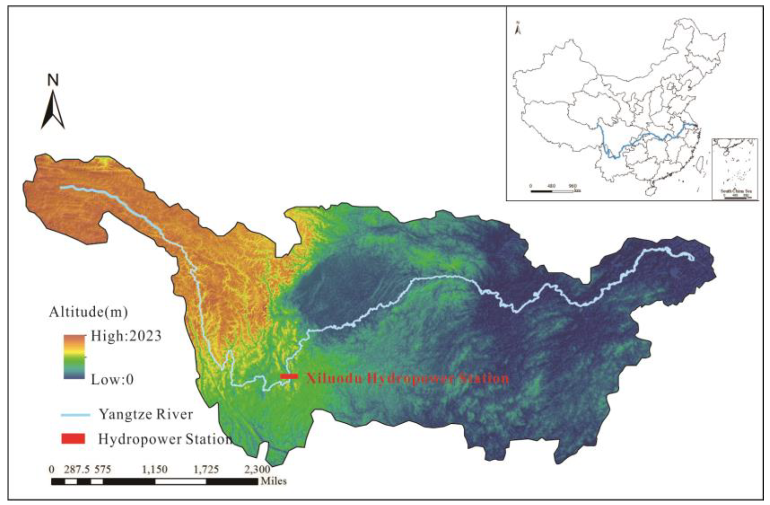
Given the above, in this study, we consider the Xiluodu (XLD) reservoir as the research object. The XLD hydropower station is located by the Jinsha River near the upstream of the Yangtze River, and is the backbone project of China’s west–east power transmission (
Figure 1). The XLD hydropower project is mainly designed for power generation with consideration of flood control, navigation and other benefits. XLD is a large-scale water project with the total storage of 12.8 × 10
9 m
3, the regulating storage is 6.46 × 10
9 m
3, the total installed capacity is 13.86 GW. Combined with previous research results, in this study, we choose three deep learning models, i.e., RNN, long short-term memory (LSTM), and gated recurrent unit (GRU) developed from RNN, to build the reservoir operation model and predict the reservoir outflow [
20,
21,
22]. The goals of this study are (1) to discuss the effect of the parameters setting on the simulation performances for three models; (2) to explore the applicability of the deep learning model to reservoir operation simulation; and (3) to analyze the rationality of the selected influence factors and the importance of various influence factors in reservoir operation decisions.
2. Methodology
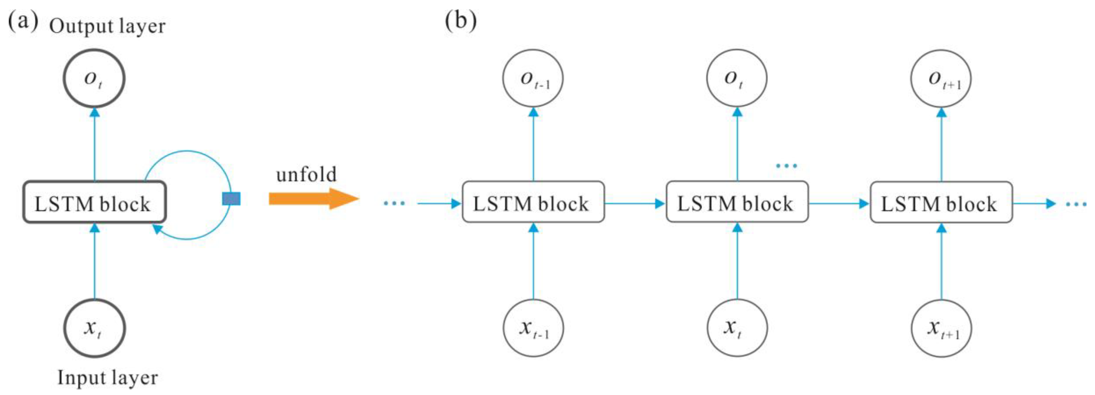
The RNN consists of an input layer, one or more hidden layers and an output layer (
Figure 2). The hidden layer continuously recurrently trains the network according to the input time of the sequence (
Figure 3). In this study, the neural network is a three-layer network structure. The input data
X (
x1, x2, …,
xi, …,
xn1) and output data
Y (
y1, y2, …, yk, …, yn3) are connected by the hidden layer
H (
h1,
h2, …,
hj, …,
hn2), where
n1,
n2, and
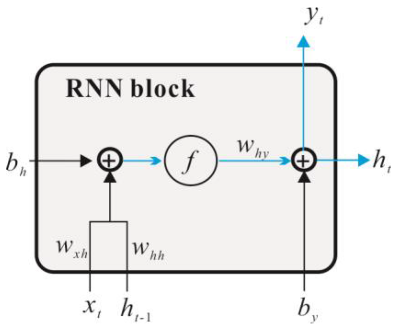
n3 represent the total number of inputs, hidden neurons, and outputs. The number of input layer and output layer nodes determined by the input and output data of the model. As an important parameter affecting the performance of the model, the number of hidden layer nodes is usually determined by a trial and error method in the training process. In this paper, the weight coefficient matrix is represented by
W (for example,
Wxh represents the weight coefficient matrix of the input layer to the hidden layer.), the offset vector is represented by
b (
bh represents the offset vector of the hidden layer), the activation function is represented by
f(), and the learning and training process of the RNN neural network is as follows:
Although an RNN can effectively deal with nonlinear time series, there are still some problems: (1) due to the problems of gradient disappearance and gradient explosion, an RNN cannot capture the temporal features especially the long-term dependencies [
22,
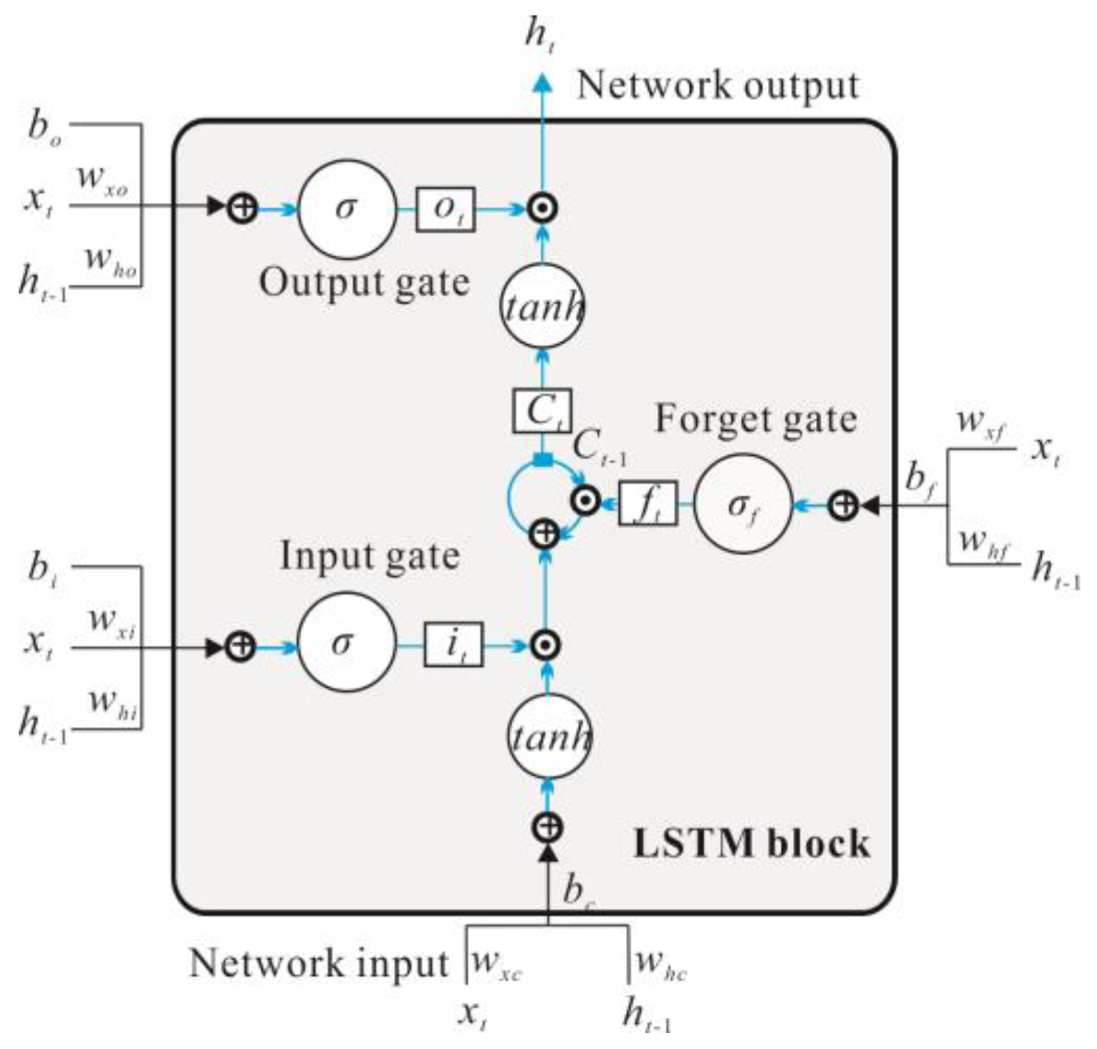
23]. The training of RNN models need to determine the length of the input sequence in advance, but it is difficult to obtain the optimal value of this parameter in practical application. To solve these problems, the LSTM model was invented. The difference between the LSTM model and RNN model is that the RNN block in the hidden layer is replaced by the LSTM block. This enables modeling a long-term memory capability [
24]. The LSTM block was obtained from Gers et al. [
21], and it consists of an input gate, a memory cell, a forget gate, and an output gate, as shown in
Figure 4. The corresponding forward propagation equations are presented below. The first step in our LSTM is to decide what data should be removed from the cell state. This decision is made by a sigmoid layer called the forget gate. The forget gate will generate an
ft value between 0 to 1, based on the previous moment output
ht−1 and current input
xt to decide whether to let the information
Ct−1 that is produced in the previous moment pass or partially pass, which is depicted by Equation (3):
The second step is to decide what new data will be saved in the cell state. This has two parts: first, the input gate determines which values will be updated. Next, the memory cell creates a vector of new candidate values
Ct, which can be added to the state. Later, the values produced by these two parts will be combined to update:
The final step is to determine the output of the model. First, an initial output is obtained through the sigmoid layer (output gate), and then the
Ct value is resized to −1 to 1 through
tanh and multiply it by the output of the sigmoid gate so that we only output the target parts:
In Equations (6) and (7), f, i, C, o and h are the forget gate, input gate, cell, output gate, and hidden output, respectively, and σ and tanh represent the gate activation function (the logistic sigmoid in this paper) and the hyperbolic tangent activation function, respectively, W represents the corresponding weight coefficient matrix.
In addition, the LSTM model has evolved many variants where one of the most successful is the GRU proposed by Chung et al. [
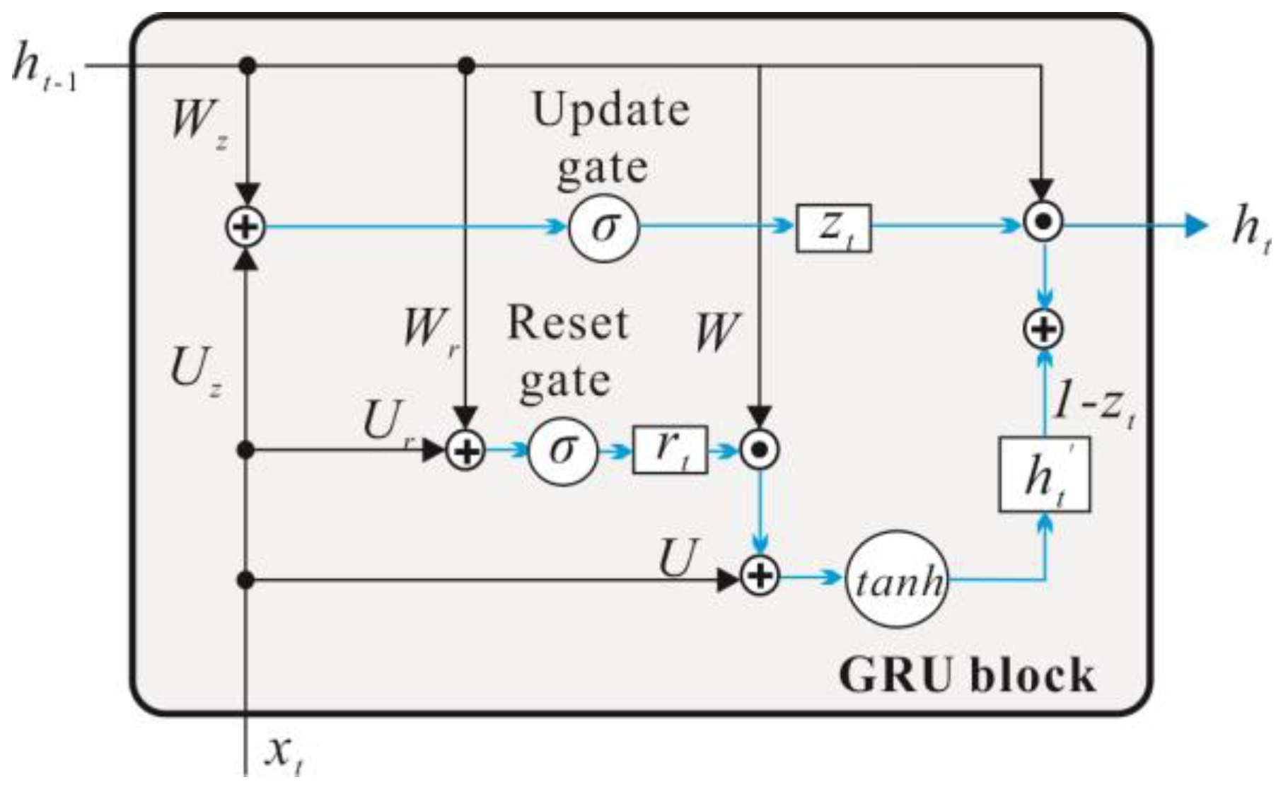
20]. GRU is a simplified version of LSTM, and its principle is similar to LSTM, which controls input, memory, output, and other information data through a gating mechanism. The main change corresponds to the replacement of the input gate, the forgetting gate, and the output door of the LSTM cell with upgrading of the gate and reset gate combined with the cell state and the output (
Figure 5). The main calculation process is as follows: firstly, the status of the hidden layer cells is updated by the update gate and the reset gate:
Next, the memory cells generate the memory contents of the hidden layer at current moment:
Finally, the hidden layer output of the current moment is calculated:
In Equations (8) and (11), z, r, h’, and h are the update gate, reset gate, hidden memory, and hidden output, respectively. Herewith, σ and tanh represent the gate activation function (the logistic sigmoid in this paper) and the hyperbolic tangent activation function, respectively. W and U represent the corresponding weight coefficient matrix.
The training process of three models adopts back propagation through time (BPTT), a principle that is similar to the classical back propagation (BP) [
25]. The main training process is as follows: Firstly, the output values of hidden layer cells are calculated according to the forward calculation method. Secondly, the error values of hidden layer are calculated on the basis of back propagation of time step and network structure. Furthermore, the gradients of each weight are calculated according to the corresponding error terms. Finally, the weight coefficients are updated by adaptive moment estimation (Adam) algorithm. Therefore, for the selected three neural networks, the number of iterations is one of the main parameters affecting the model performance similar to a BP neural network.
In addition, for the deep learning model, the batch size is also an important parameter that affects the model performance. Batch size represents the size of the data volume, namely, the number of training samples in an iteration. Then the model updates the network parameters (weight and bias) by calculating the error between actual output value and expected output value of the sample set.
3. Model Building
In this study, we collected the hourly operating data and meteorological data of XLD reservoir from 30 June 2014 to 31 December 2017 (every four or six hours, a total of 6000 records of data). The operating data include the inflow and outflow of the reservoir, the water level upstream and downstream of the dam [
26] and the meteorological data include precipitation, evaporation, atmospheric temperature and relative humidity [
27]. Based on the commonly accepted “80/20” split rule, the data from 1 January 2016 to 31 December 2017 are used as the test period and the remainder is used for training. The reservoir operating data and meteorological data are imported as the model inputs (decision variables) and output (target variable). Specifically, the inputs include current time (month of year, hour of day), current inflow (one-moment lag), previous outflow (one-moment lag), current highest operating water level, current lowest operating water level, current time (month of year, hour of day), and firm output of the hydropower station (
Table 1). The output of model is current outflow. The model used in this paper presents three recurrent neural networks: simple RNNs, LSTM, and GRU.
To explore the effect of parameter setting on model performance, different parameter combinations are tested. The results of previous studies show that the main parameters affecting the model performance mainly include batch sizes, the number of maximum iteration and hidden nodes, where the batch sizes mainly affect the calculating speed [
28]. First, the batch sizes were fixed at 500, and then we tested the influence of the iteration and hidden node on the simulation performance. The number of hidden nodes and maximum iterations rages from 5–100 with a set interval of 5, for a total of 400 working conditions. Then, according to the experimental results of the previous step, under the appropriate parameters setting condition (the number of hidden nodes and maximum), we adjust the batch sizes to test the effect of the batch sizes on model performance. The batch sizes ranges from 1–800. Within a range of 1–100, the interval is 5, within a range of 100–800, the interval is 25, for a total of 44 working conditions.
Finally, combining the study results of parameter setting, we set the parameter values of each model for keeping consistency of model convergence. At the same time, in order to reduce the randomness error, we set the training frequency to 10, and repeat train three models to calculate the mean value of the simulating results. In addition to the global precision, the simulation effect of the models on different hydrological periods is also considered. Combined with historical hydrological data, the flood season of XLD hydropower lasts from July to September, and the water supply season lasts from December to May of the following year.
4. Results and Discussion
4.1. Comparison of Parameter Sensitivity and Model Performance
In order to compare the simulation performance of three models under different parameter setting, we select the mean square error (
RMSE), root mean square error and standard deviation ratio (
RSR) and the Nash–Sutcliffe efficiency coefficient (
NSE) as the model accuracy evaluation index. Furthermore, the time consumption is used as the basis for evaluation of the speed of the model to explore the influence of parameter setting on model precision and calculation speed. The calculation method is shown in Equations (12)–(14):
where
si represents the model simulation value,
oi represents the observed value, and
represents the average value of the observed value. The indices
RMSE and
RSR are valuable because they indicate the error in the units (or squared units) of the constituent of interest. The
NSE is a normalized statistic that determines the relative magnitude of the residual variance compared to the measured data variance [
29]. As suggested by previous studies, an
RMSE value less than half the standard deviation of the observed data may be considered low, and if
RSR < 0.7 and
NSE > 0.5, model performance can be considered satisfactory, whereas an
NSE value <0.0 indicates that the mean observed value is a better predictor than the simulated value, which indicates unacceptable performance [
30,
31,
32].
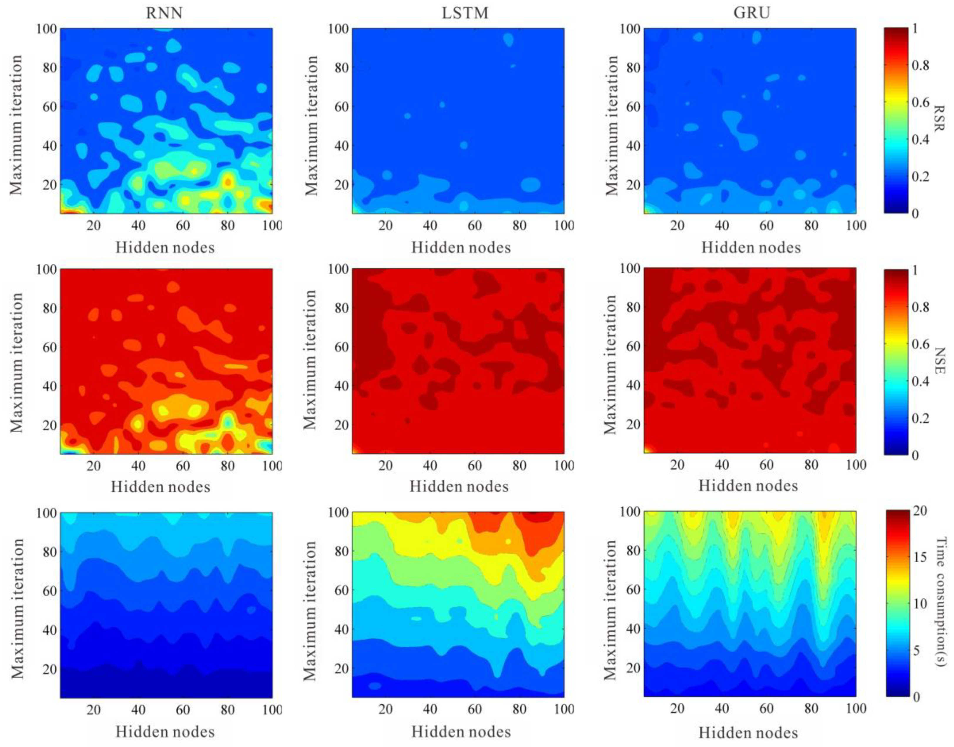
First, we explore the influence of the number of iterations and hidden nodes on the model performance. The performance optimization surface of different parameters and network models is shown in
Figure 5 and
Figure 6. The results show that with the increase of maximum iterations the accuracy of three model increases, the time consumption increases. Additionally, an increase in the number of maximum iterations does not significantly improve model precision when the number of maximum iterations reaches a certain limit (
Figure 6 and
Figure 7). The effect of the number of hidden nodes on the model performance is more random. With the increase of the number of hidden nodes, the model precision and calculation speed show an irregular rise or decrease (
Figure 6 and
Figure 7). In advanced investigation, we deduced that the training method of BPTT uses a forward algorithm to calculate the output value, and a backward algorithm to calculate the error of each hidden cell. We continuously update the network weight extending the direction of error reduction. Therefore, after the training reaches a certain limit, the increase of the number of iterations is no longer significant for the improvement of the model precision. The influence of hidden nodes on model precision has always been a key problem in artificial neural network research. Yao [
33] indicates that as an important structural parameter of artificial neural networks, the hidden nodes are very important to the accuracy of model. However, the relationship between the number of hidden nodes and the precision of the model has not been established. It is generally considered that the selection of the number of hidden nodes is related to the number of input layer nodes and the number of output layer nodes. In the practical application, the optimal number of hidden nodes can be set by a trial and error method [
34,
35].
In detail, with respect to each model, the performance of RNN model is significantly influenced by the number of iterations and hidden nodes, and the accuracy of the model increases rapidly with the increase of iterations. When the number of iterations is greater than 60, the model is more likely to obtain high precision (
Figure 5 and
Figure 6). The influence of hidden nodes on the simulation accuracy and calculation speed is not obvious, however, the research results show that if the number of hidden nodes is less than 20, the required iterations for model convergence is fewer (
Figure 5 and
Figure 6). Compared to RNN models, the LSTM and GRU models are less affected by the number of iterations and hidden nodes. Meanwhile, the convergence speed and calculation speed of these two models are fast (
Figure 5 and
Figure 6). When the number of iterations is greater than 20, the model can obtain high precision prediction results (
Figure 5 and
Figure 6).
Second, we further explore the effect of the batch sizes on model accuracy and calculation speed (
Figure 8). To ensure the high-precision prediction results of the model, we set the number of maximum iterations to 100 and the number of hidden nodes to 10 for all three models. As shown in
Figure 8, the batch size mainly affects the calculation speed of the models. With the increase of the batch sizes the calculation speed of three models increases significantly. This has been proved by previous studies which have shown that batch sizes are the main factor that limits the computational speed of the models [
28,
32]. On the other hand, the effect of batch sizes on model precision is low. According to previous studies, the smaller the batch sizes the greater the randomness in one batch and the less likely the model is to converge. However, due to the large randomness, it is easy to obtain the global optimal value. On the contrary, the bigger the batch sizes the more features of data can be represented. Furthermore, the more accurate the gradient descent direction the faster is the model converges with the calculation speed of the models will be improved. However, the large batch size possesses a relative lack of randomness, and it is easy to keep the gradient falling in one direction and fall into the locally optimal solution.
In conclusion, for the selected three deep learning models, we believe that the effect of maximum iterations on model precision should be firstly taken into account. Nevertheless, the effect of hidden nodes on model precision is weak and can be considered later. Furthermore, a reasonable increase in the number of maximum iterations is helpful to improve the accuracy of the model. On the other hand, the batch sizes mainly affect the calculation speed of the model, while the larger the batch sizes the faster the calculation speed. However, the large batch sizes easily cause a local optimal solution for model, reducing the accuracy of the model. Finally, the parameter values required for model convergence are not only related to the model itself, but also limited by the data structure and data volume of the training set. We cannot give the certain values for the optimal parameters of different models and datasets. We suggest that prior to the practical application the parameters should be adjusted continuously based on the data, while the parameter setting rules given in this paper are designed to obtain the best simulation result.
4.2. The Applicability of the Model in Reservoir Operation
4.2.1. Model Performance Index
During the reservoir operation, it is often necessary to predict the outflow of the current moment based on the reservoir inflow to guide the reservoir operation. Therefore, besides the prediction of outflow, the model also should be able to simulate and predict the outflow trend of the reservoir, as well as to capture the details, such as the sudden flood peak during the flood season and extreme low inflow during the dry season. Therefore, in addition to the global precision, the simulation effect of the dry season and flood season is also compared and analyzed. Combined with the above research results, the number of maximum iterations is uniformly set to 100, the number of hidden nodes is 10, and the batch size is 50. For the model convergence, the simulation results are compared and analyzed in light of three aspects of model accuracy, uncertainty, and time consumption. The applicable scenarios of each model are discussed.
First, the simulation accuracy of each model is compared and analyzed. As suggested by Moriasi et al. [
30], an
RMSE value, which is less than half of the standard deviation of the observed data may be considered low. If
RSR < 0.5 and
NSE > 0.75, the model performance can be considered satisfactory, whereas an
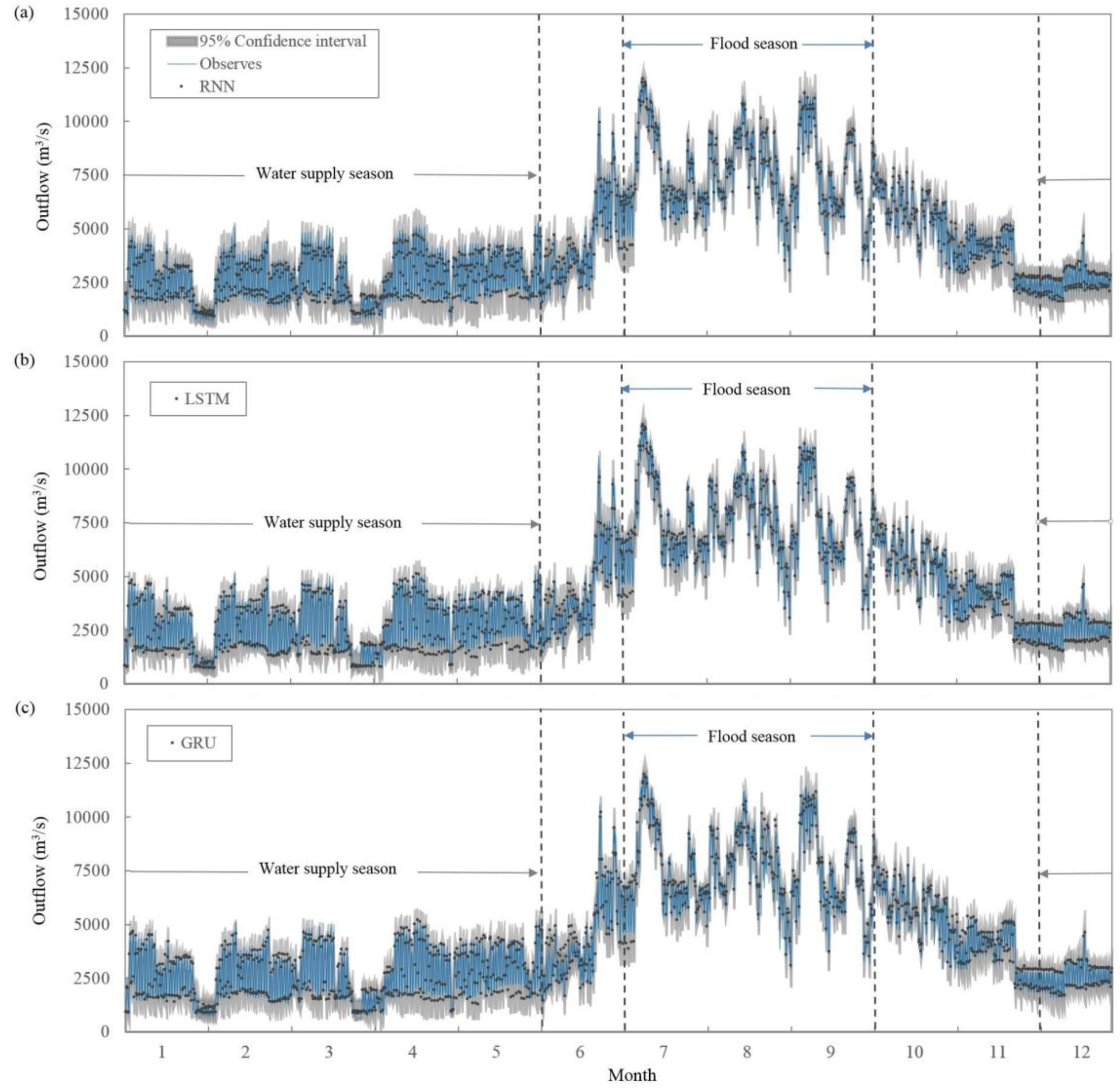
NSE value < 0.0 indicates that the mean observed value is the better predictor than the simulated value, which indicates unacceptable performance. Therefore, with respect to global accuracy, all three models can complete the prediction performance of reservoir outflow, and the comparison among three models shows that the global accuracy of LSTM model is higher than that of GRU and higher than that of RNN, but the difference is low (
Figure 9,
Table 2). In addition, for the flood season, the best accuracy of models rank as LSTM > GRU > RNN. Herewith, during the water supply season, the best accuracy of models rank as LSTM > RNN > GRU. Meanwhile, the difference test of multiple simulation results of the model showed no significant difference (
Figure 9,
Table 2).
Next, this paper further analyzes the uncertainty of three models. The width of the confidence interval is one of the commonly used evaluation indices of the model uncertainty. For the specified confidence level, for ensuring high coverage, the lower the width of the interval and the lower the uncertainty of the model the better the simulation effect can be observed. Our experimental results show that 95% confidence interval can cover the measured values of outflow well for the three models (
Figure 9). At the same time, the comparison among different models shows that the interval width of the models is close to each other, and the difference of uncertainty is small (
Figure 9).
Last, we evaluated the performance of three models from the time consumption. The results show that the calculated speed of the three models is very fast while the whole process of training and forecasting can be completed within ten seconds. Thus, it can meet the requirement of high-speed decisions for short-term reservoir operation (
Table 2). The comparison among different models shows that the time consumption of LSTM is higher than that of GRU and higher than that of RNN (
Table 2). According to our analysis, the reason for this result is the difference in the hidden cell structure of the model. Furthermore, the hidden cell structure of RNN model is simple, therefore, the calculation can be performed over the faster. LSTM adds multiple "control gate", therefore, the calculation process is more complex than RNN and the time consumption is increased. GRU is a simplified variant of LSTM, which continues LSTM’s concept of "control gates", but the number of “control gate” is reduced, and the hidden cell structure is simpler than LSTM with the decreased time consumption.
To sum up, the three models consider the influence of influence factors on reservoir operation with the precise capturing of the sudden flood peak during flood season and extreme low inflow during dry season, ensuring the flood control at the flood season and water supply at the dry season. In addition, the models are easy to use by management personnel with lower professional levels. This simplifies the operation and management of hydropower stations. Therefore, from the perspective of model performance, we believe that these three models built in this paper on the basis of deep learning might be useful during reservoir operations.
4.2.2. Model Economic Index
In addition to the requirement for model performance, the reservoir operating model should also meet the reservoir operating rules and possess the comprehensive benefits of the reservoir. Given that the main operating obtain of XLD hydropower is flood control and power generation, this paper focuses on the flood control and power generation benefits of the reservoir operating models. As shown in
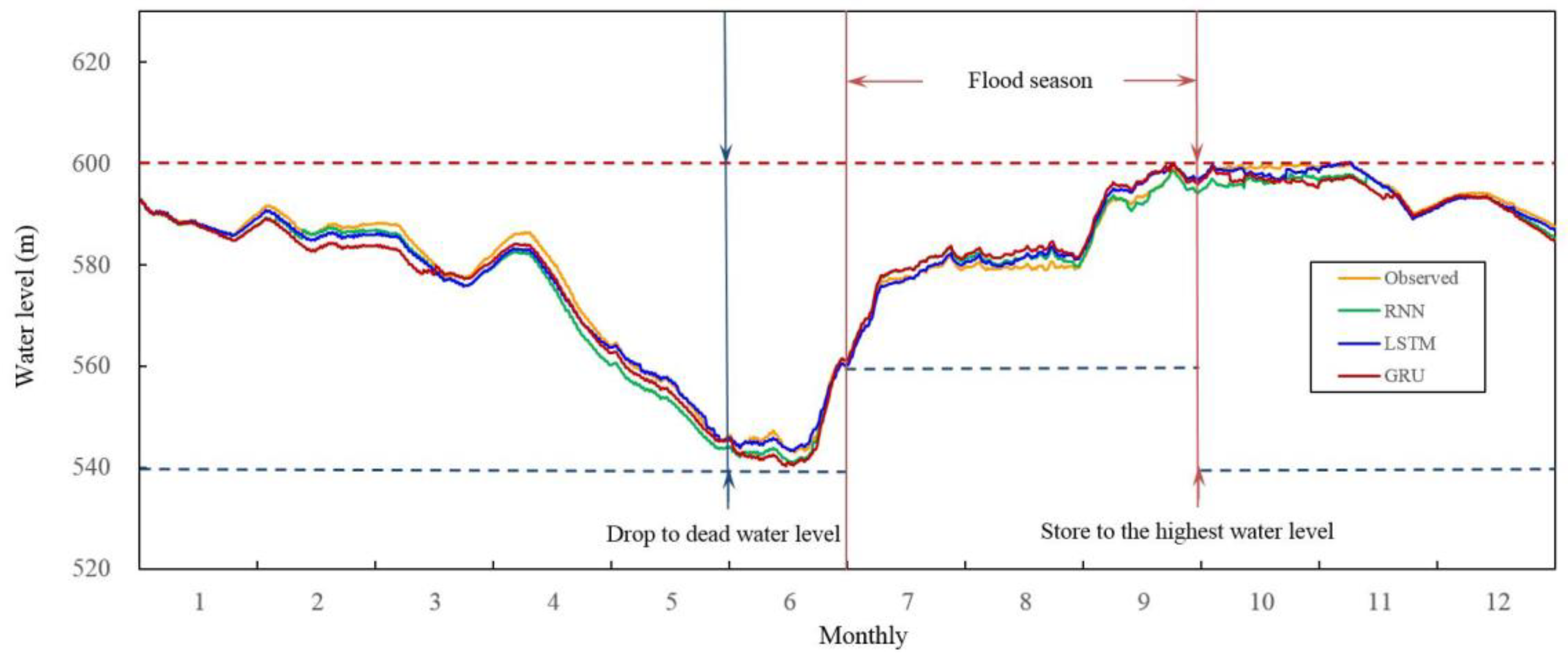
Figure 10, according to the rules of XLD hydropower station, the water level of the reservoir should be between the dead water level of 540 m and the normal highest water level of 600 m. During the flood season (from 1 July to 30 September), the normal water level should be between the limited flood water level of 560 m and the normal highest water level of 600 m. From October to November, the reservoir keeps the operation at a high-water level. Starting from December, the reservoir operates at a water supply season, and the water level should be gradually decreased. The water level at the end of the water supply season (the end of May) should not be lower than the dead water level. Our research results show that the simulation results of the selected three deep learning networks can meet the water level limitation requirements of XLD reservoir under different operating seasons and implements the flood control and water supply functions of the reservoir (
Figure 10).
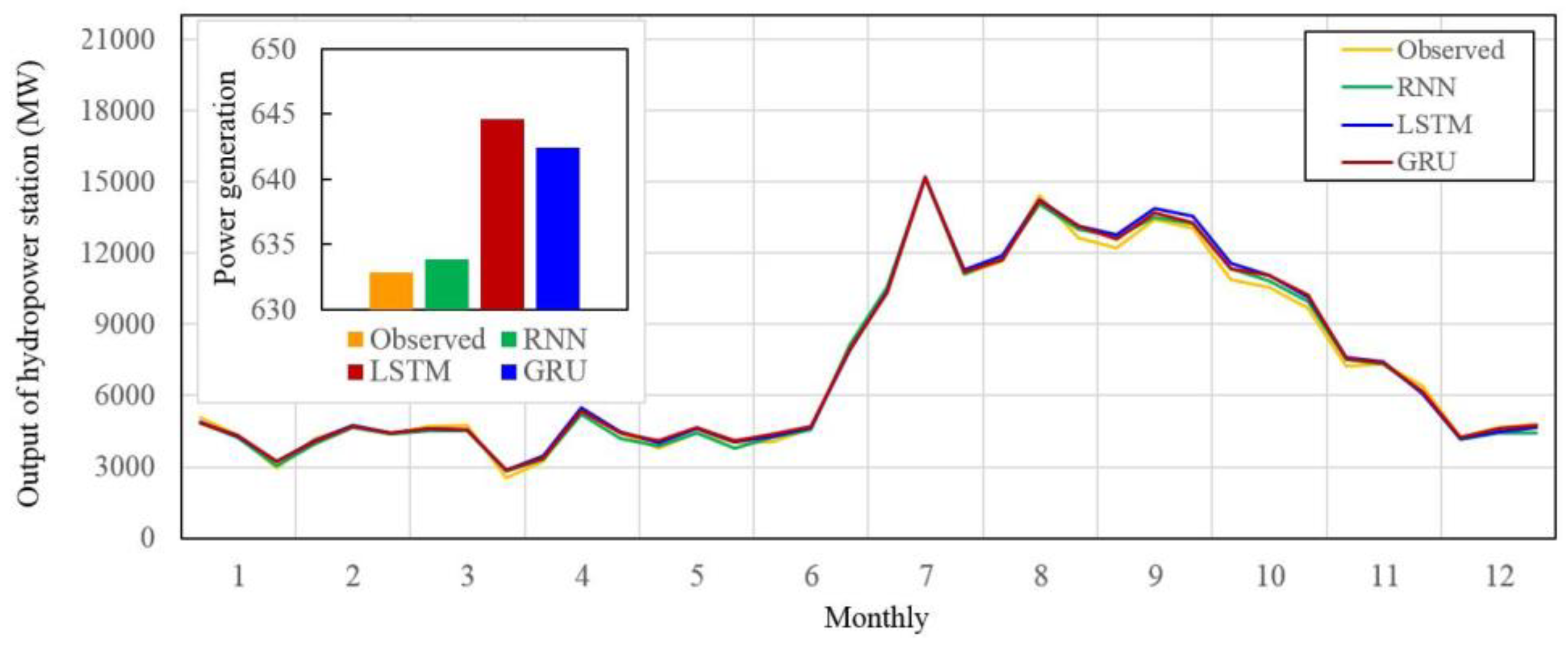
On the other hand, our study also analyzes the power generation efficiency of the simulation results, and the results show that the simulation results of three models can complete the power generation task of XLD reservoir. The obtained power generation is similar or slightly higher than the measured results (
Figure 11). It is shown that the three models constructed in this paper may learn the reservoir operating rules from the historical operating data, whereas the operating scheme meets the reservoir operating rules and implements the flood control and power generation targets of the reservoir. All three models can be used for actual reservoir operation.
4.3. Importance Analysis of Input Factors
Reservoir operation is a complex problem affected by many factors. This paper builds three deep learning models for reservoir operation based on the historical data and meteorological data of the reservoir. For the analysis of the effect of each decision factor on the decision variables of reservoir operation, regression analysis is carried out for the decision variables and influence factors of the reservoir. The results showed that the explanation degree of selected influence factors for the decision variables during the whole year (97.9%) and flood season (97.6%) are greater than during the water supply season (91%) (
Figure 12). This shows that the influence factors selected by us are reasonable and can explain the most changes of reservoir outflows. Meanwhile, due to the fact that some updated information of outflow has not been explained especially at the water supply season, we should consider the influence factors more comprehensively in the later work and study those factors that may affect the reservoir scheduling decision to add to our model. It would help to improve the prediction accuracy of the models.
On the other hand, for the further analysis of the influence of influence factors on the model, we conducted a sensitivity analysis of the relationship between the influence factors and decision variables. Sensitivity analysis is the process of defining model output sensitivity for change of the input variables. Sensitivity analysis is a simple procedure that is applied after the modeling phase, and it analyzes the model responses when the inputs are changed. In this work the sensitivity in accordance with variance was used to compute the relative importance of the input variables for the three selected models [
36]. Meanwhile, in view that the number of influence factors in this paper is large, the influence factors are divided into four categories (time information, runoff and water level information, meteorological information, and hydropower firm output information; see
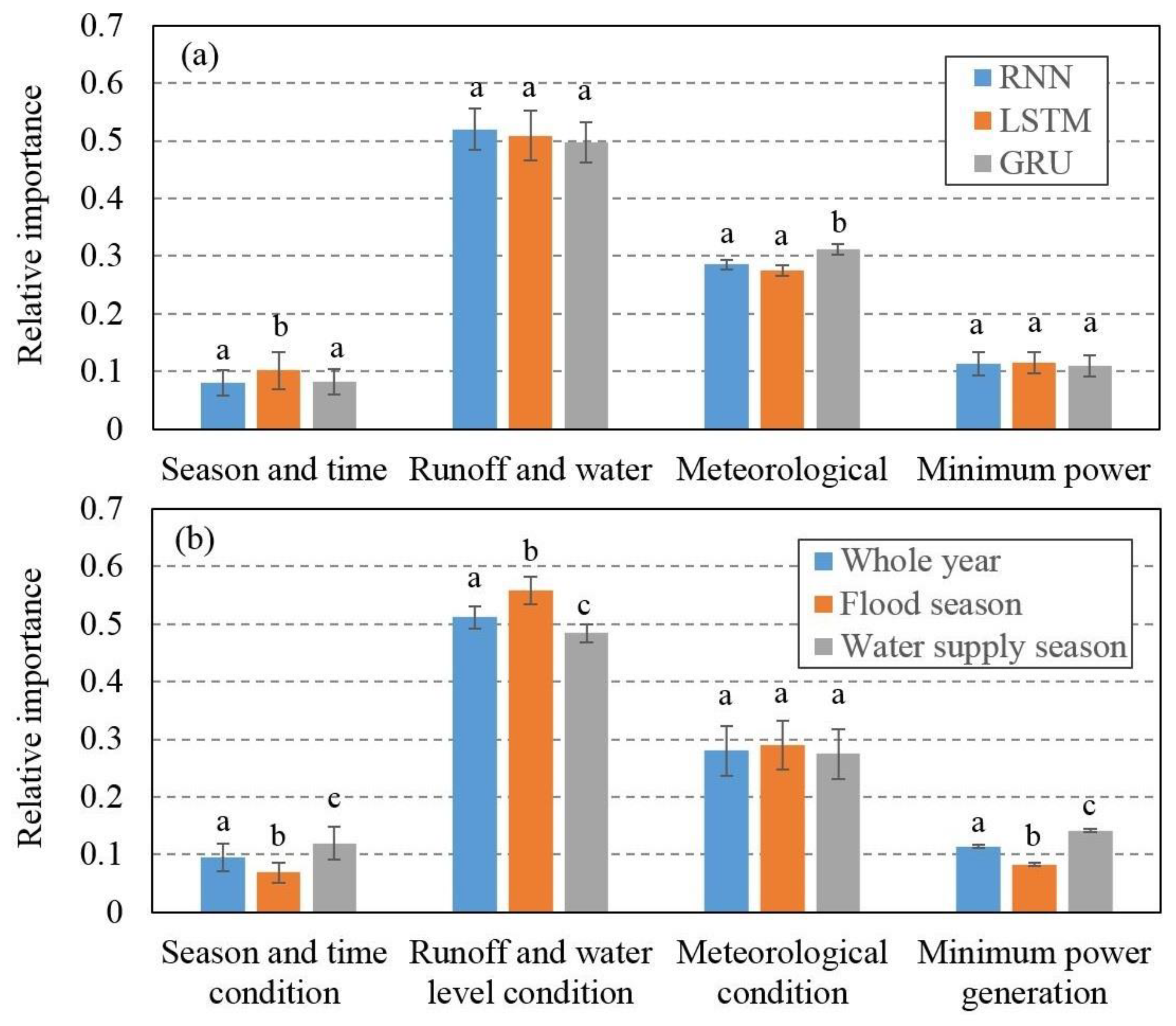
Table 1 for details) for the more accurate analysis of the impact of different influence factors on model output results. The analysis results are shown in
Figure 13. First, for the influence of influence factors on the model output, there is a small difference among three deep learning models. Overall, the most informative variable for the model to predict outflow is runoff and water level condition and meteorological condition followed by season and time condition and minimum power generation (
Figure 13a).
For different operating season, the influence of influence factors on decision variables is quite different (
Figure 13b). Runoff and water level information are the main influence factors affecting reservoir operation during any operating season (
Figure 13b). Meteorological information is the second most important decision factor influencing the output of the models. The relative importance of meteorological information in the flood season is 0.33, while the relative importance of meteorological information during the whole year and the water supply period are slightly lower than those of the flood season, both of which are 0.28 (
Figure 13b). The reason for the above difference is that the meteorological conditions mainly affect the reservoir operation by influencing the reservoir inflow conditions. During the water supply season, the precipitation, temperature and evaporation values are low, so the influence on the inflow is small, and the effect on reservoir operation is relatively low. For a reservoir with a power generation function, the firm output information is also one of the important factors influencing the decision of reservoir operation. Our analysis results show that the relative importance of firm output information during the water supply season is as high as 0.14, and the relative importance of firm output information is 0.11 during the whole year and is 0.08 at the flood season (
Figure 13b). This may be associated with the cause that, during flood season, the hydropower station should not only ensure the power generation, but also should facilitate the flood control function. Therefore, the explanation degree of firm output information for model output is relatively low. Time information is an important parameter for ensuring that the model can describe different operating rules for different operating seasons. Our research results show that the relative importance of time information for the output results of the model is 0.10 during the whole year. The flood season is 0.07, and the water supply season is 0.12 (
Figure 13b). According to our analysis, the possible reason for this result is that the time information consists of two parts: the monthly results and daily results. The monthly information mainly associated with the model to learn the operating rules for different seasons, and the daily time information contributes to the model with the daily peaking operation of the reservoir. During the flood season, due to the flood control task of the reservoir, the peaking operation is relatively less than that of the water supply season and during the whole year. Thus, the importance of time information for the flood season is slightly lower than that of the water supply season and during the whole year.
In conclusion, the selected input factors explained most of the reservoir outflow changes. During the different operating seasons the explanation degree of various input factors on reservoir outflow is different. However, the runoff and water level information are always the main influence factors that affect the reservoir operation.
4.4. Model Generalization Analysis
This paper conducted a case study on XLD reservoir to explore the applicability of deep learning algorithms in reservoir outflow simulation. The results show that the three constructed models can learn the reservoir operating rules well from the historical operating data and give the operating scheme that meets the reservoir operating rules, as well as provide the flood control and power generation targets of the reservoir. However, since the operation time of the XLD reservoir is short (built in 2014) and the inflow of the XLD reservoir is regulated by the upstream reservoir, there are few extreme inflow scenarios in the actual operation of XLD. This also results in the model training data set not including extreme inflow events, so the model training fails to take extreme inflow conditions into account. In addition, the lack of generalization ability has always been the focus of traditional neural networks. Therefore, whether the deep learning network constructed in this paper can cope with extreme inflow events has become a key issue to be considered in the practical application and promotion of the model. In this paper, we discussed this problem on the basis of previous research results, from the following three aspects:
First, the performance advantage of the deep learning model. Deep neural networks have good pattern learning ability and memory ability, and it shows the generalization ability that is much better than the traditional ANN. Traditional neural networks believe that the model memory on training data is an important reason for the poor generalization ability. Therefore, a variety of regularization methods are often used to reduce the model memory. However, the current research shows that deep learning networks have both good memory and generalization ability. The regularization method is helpful to reduce the generalization error, but even without this method the model can still be well generalized [
37].
Second, the reservoir operation model based on physical significance is used to supplement the learning samples. The reservoir operation model based on physical significance can generate operating schemes for different inflow scenarios according to the given operating rules. However, the calculation and solution process of these models are complex and require a high professional ability of the users, which limits the practical application of such models. The deep learning network is fast in computing speed and simple in sample, and is able to quickly generate response plans for emergencies. Therefore, in future studies, we can couple the advantages of the two models, using a reservoir operation model based on physical meaning to simulate various extreme inflow scenarios and emergencies which have not yet occurred in practice so as to supplement the learning samples for the deep learning network and improve the ability of reservoir operation model based on deep learning networks to deal with various inflow scenarios.
Third, model updating and training. A significant advantage of the neural network model is that it has a strong ability of learning and updating. It can re-learn and train according to the addition of new data and continuously enhance the performance of the model. Therefore, besides using mathematical models to supplement training samples, neural networks should also update training data in a timely manner and constantly add new data samples, especially the data samples for dealing with sudden extreme events, so as to improve the prediction ability of the model.
5. Conclusions
In this paper, the prediction method of reservoir outflow based on deep learning is proposed, and the prediction models of the outflow of the XLD reservoir is constructed by using the RNN, LSTM, and GRU—three recurrent neural networks. Furthermore, the parameters of each model are optimized, and the performances of the three models are analyzed, the applicability of the recurrent neural networks in the reservoir operation being investigated. The main conclusions are as follows:
(1) The number of maximum iterations, hidden nodes, and batch sizes are the main parameters that affect the model performance. The maximum iterations and the hidden nodes mainly affect the model accuracy, and the former has more influence than the latter. Batch sizes mainly affect the calculation speed of the models. A reasonable increase in the number of maximum iterations and batch sizes will improve both the accuracy and the computational speed of the models.
(2) The three models can learn the reservoir operating rules well from the historical operating data, accurately capture the sudden flood peak during flood season and extreme low inflow during the dry season, as well as realize the flood control and power generation targets of the reservoir. The models are easy to use and require a lower professional level of management personnel, which is conducive to simplifying the operation and management of hydropower stations.
(3) In different operating seasons, the explanation degree of various input factors on reservoir outflow is different, but runoff and water level information have always been the main influence factors affecting reservoir operation.
This study proves the applicability of RNN in the field of reservoir operation. At the same time, the law of parameter setting summarized in this paper and the model architecture can provide reference for subsequent researchers. Researchers can select key influencing factors, such as model input, to build the model according to the research objects and train the model according to the law of parameters.
