Development of a Large Flood Regionalisation Model Considering Spatial Dependence—Application to Ungauged Catchments in Australia


Abstract
:1. Introduction
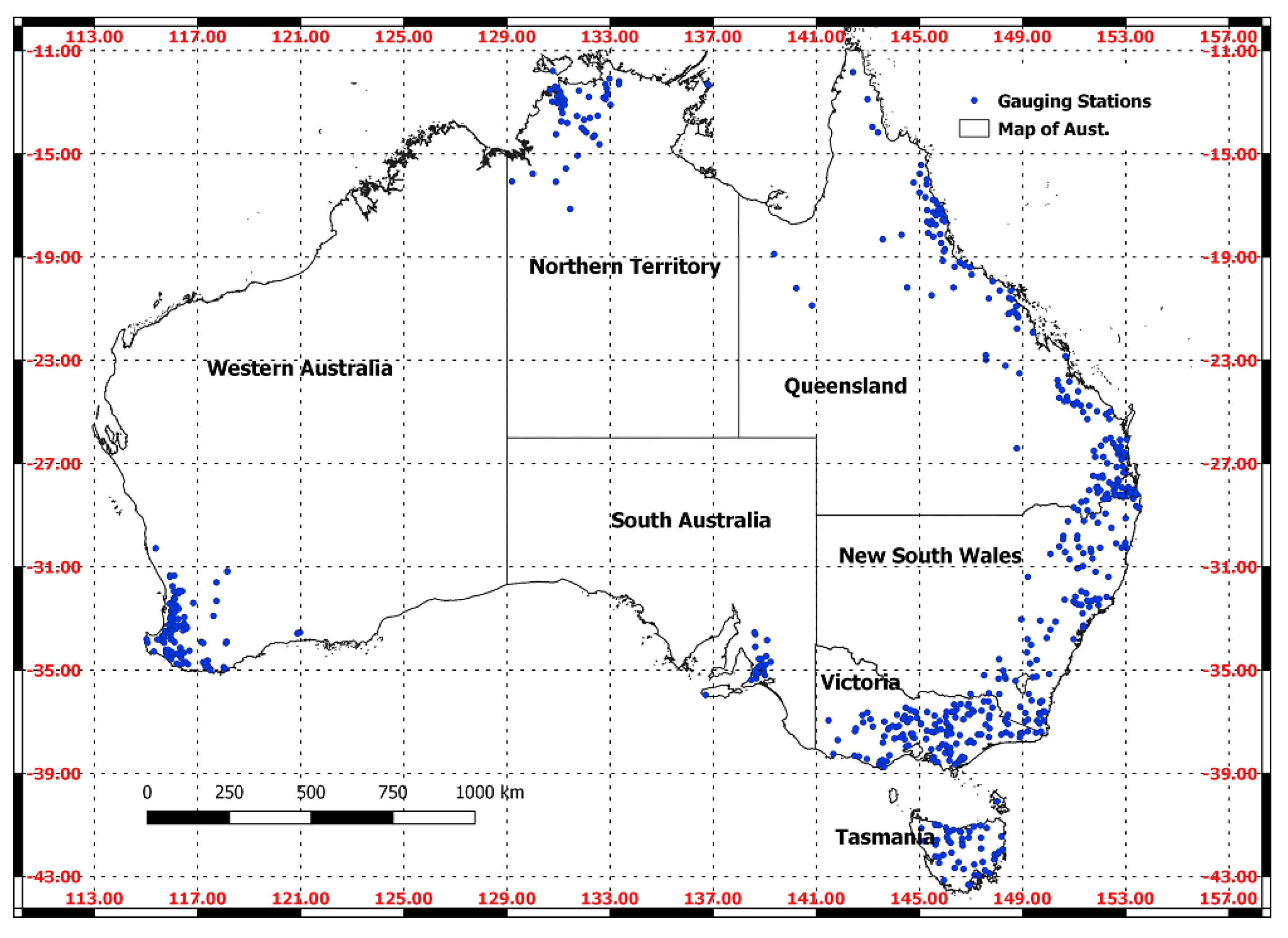
2. Data Description
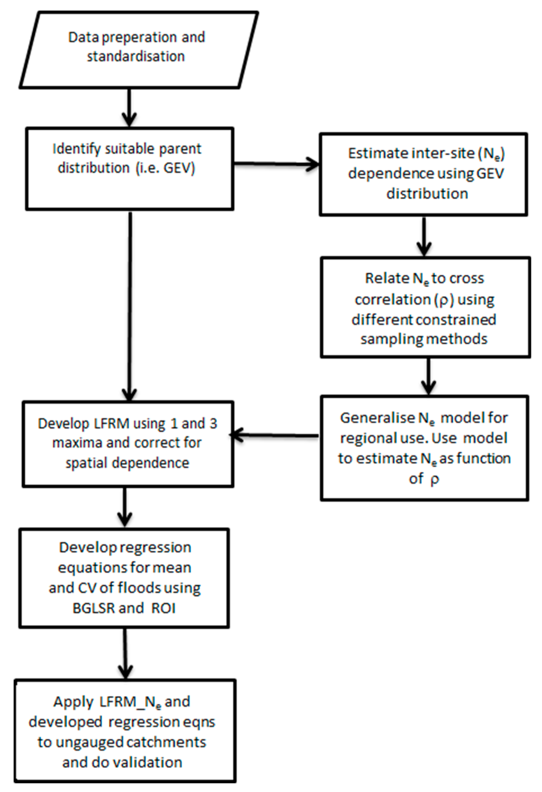
3. Methods
3.1. Identification of A Suitable Parent Distribution
3.2. Estimating Inter-Site Dependence
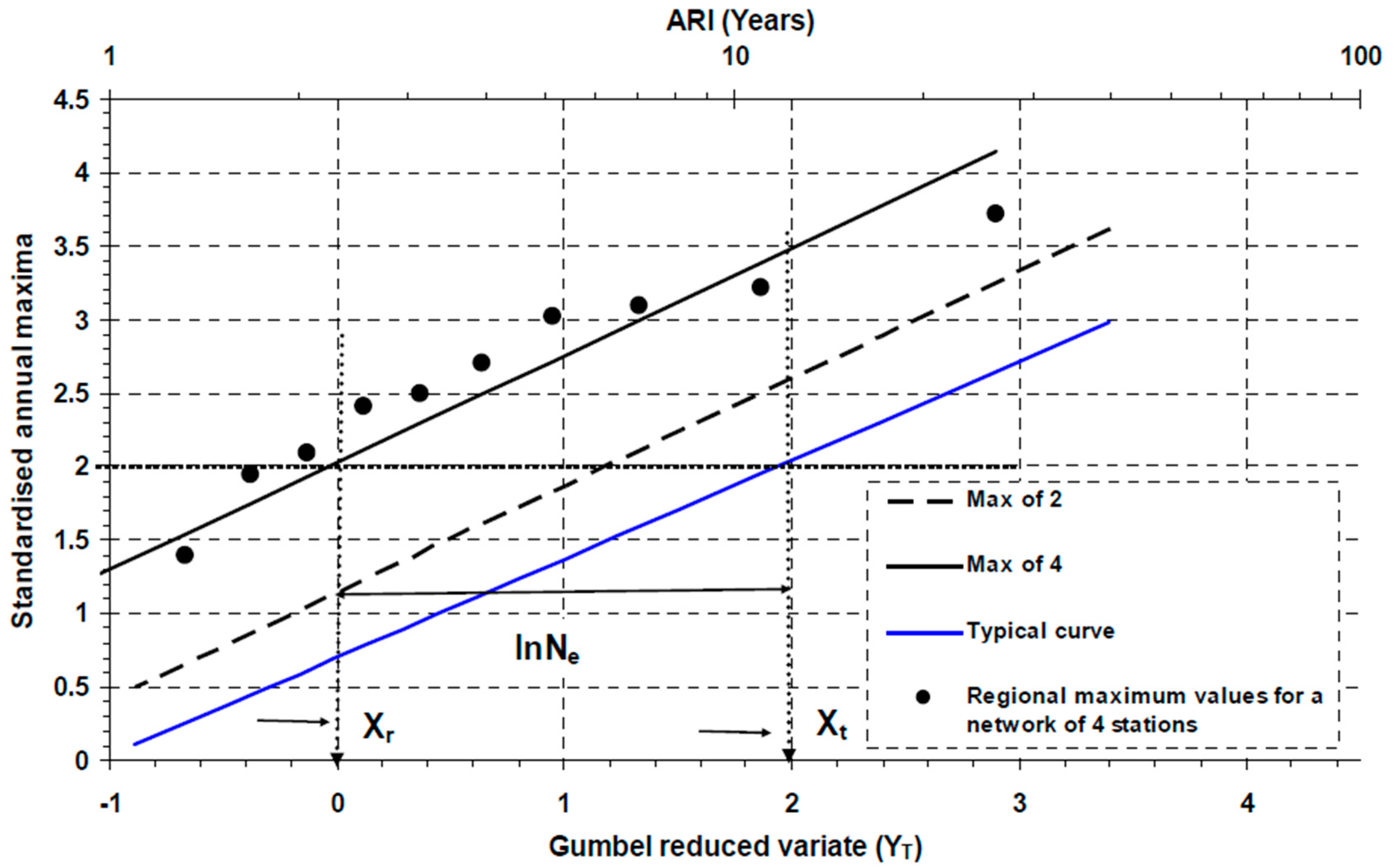
3.3. Establishing and Generalising Ne
4. Results
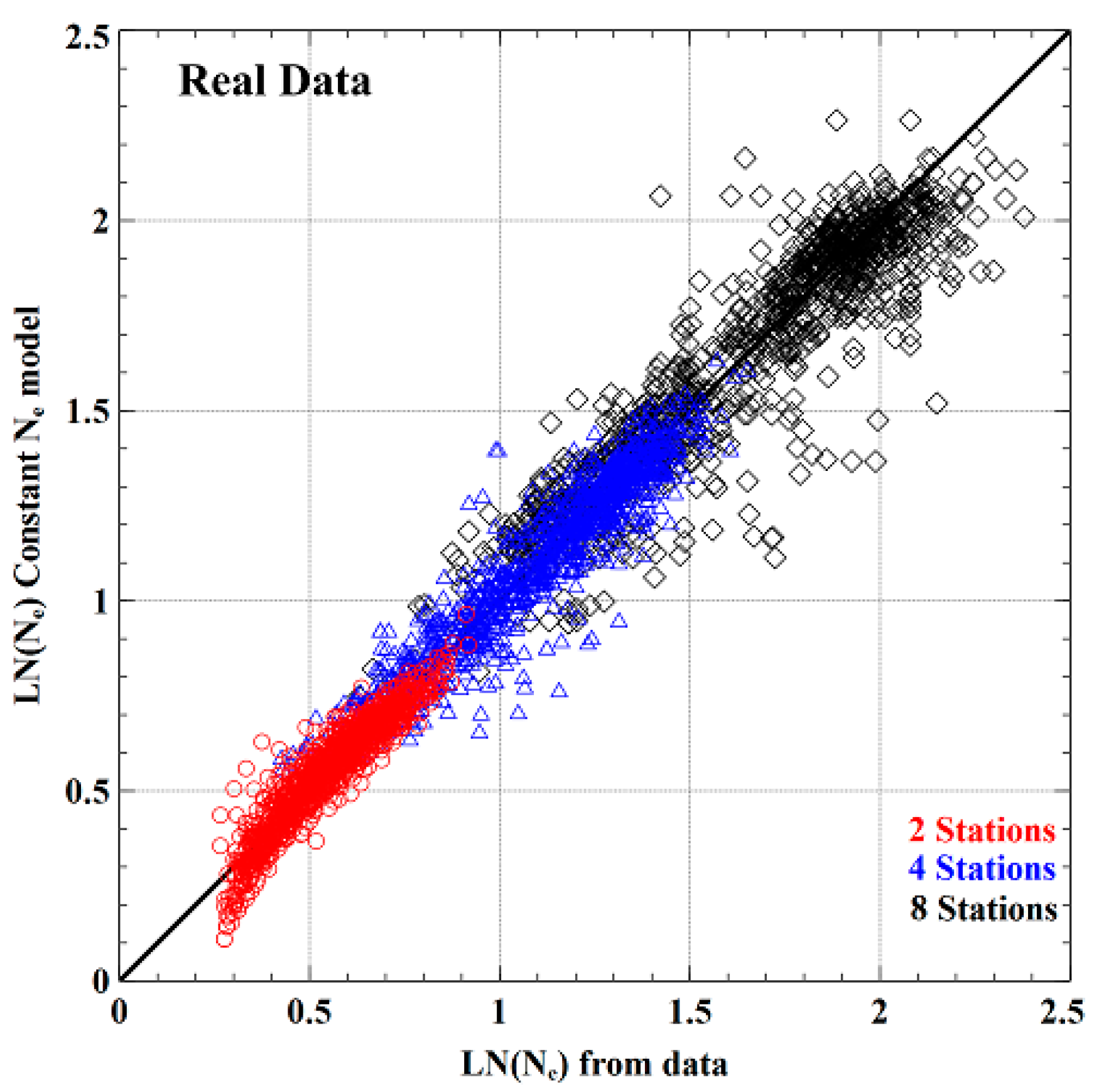
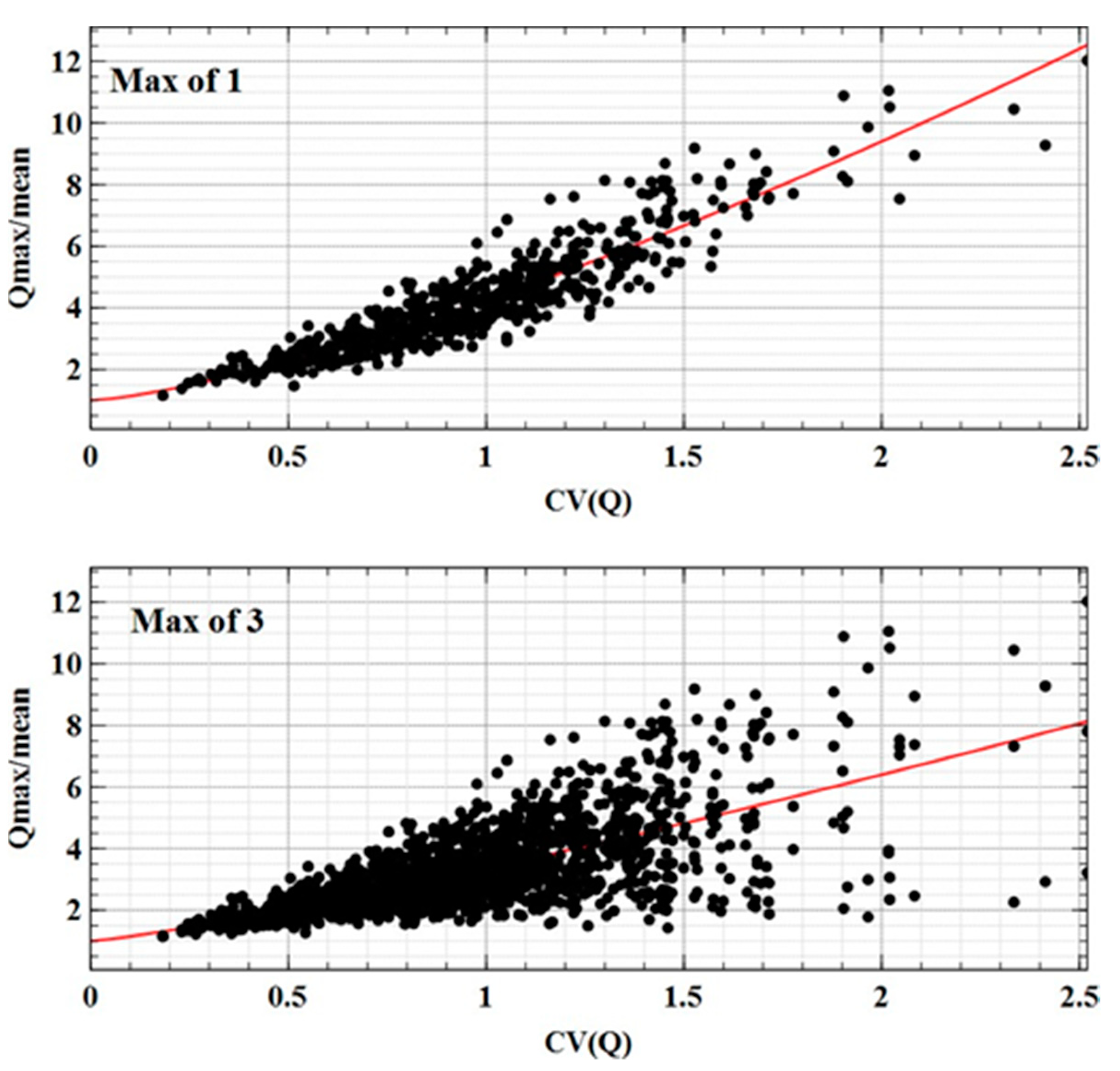
4.1. Development and Calibration of LFRM for Australian Data
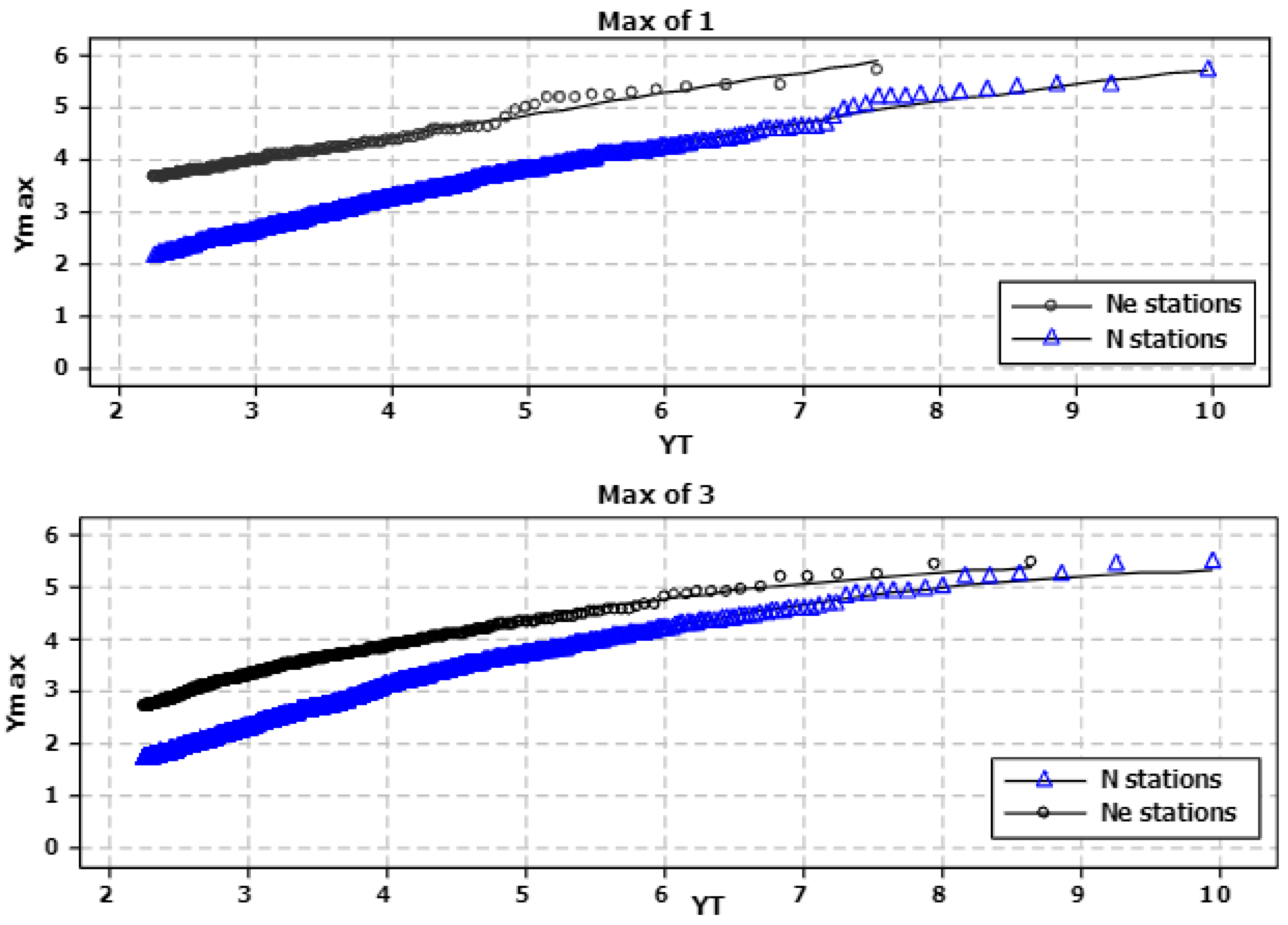
4.2. Revision of LFRM for Spatial Dependence
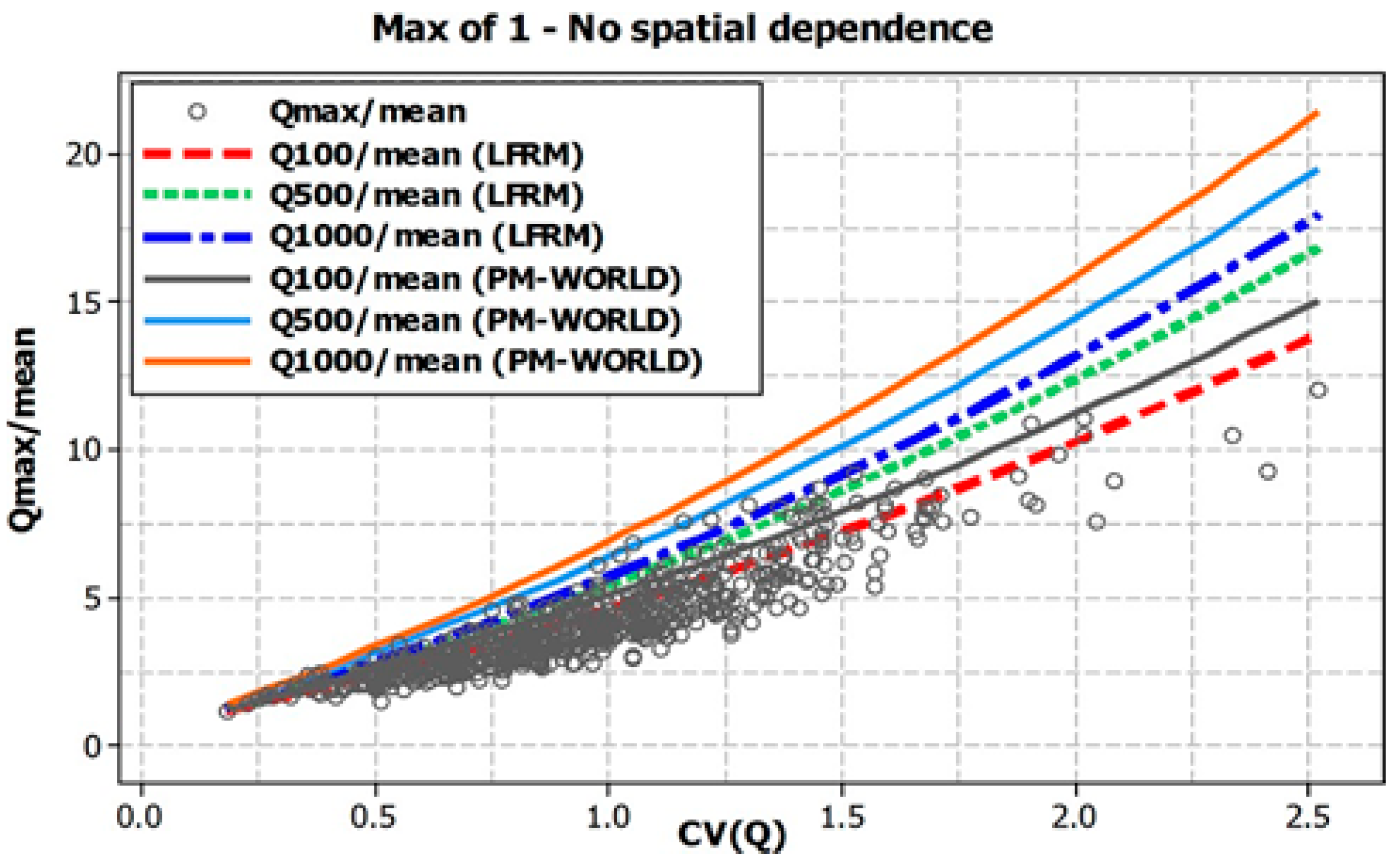
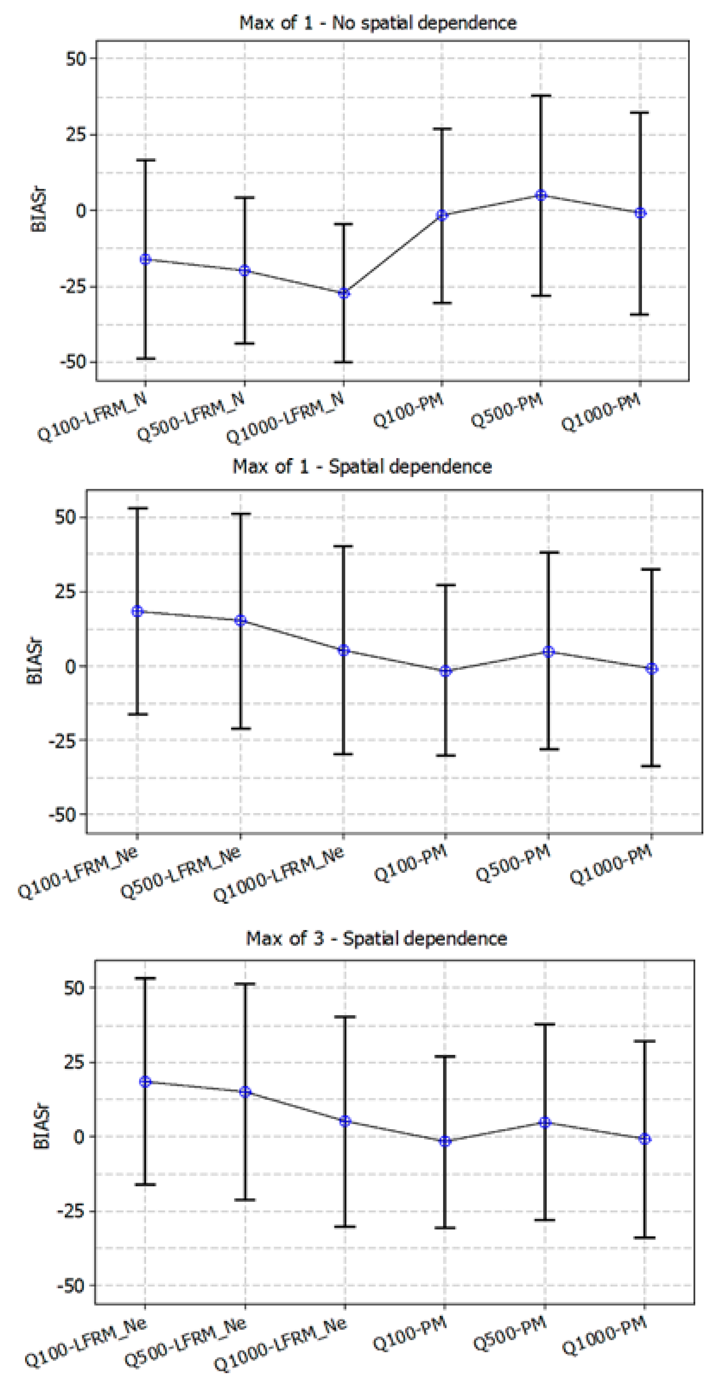
4.3. Application of the LFRM to Ungauged Catchments
5. Conclusions
Author Contributions
Funding
Acknowledgments
Conflicts of Interest
References
- Nathan, R.; Weinmann, E. Estimation of Very Rare to Extreme Floods. In Australian Rainfall and Runoff—A Guide to Flood Estimation (Book 8); Commonwealth of Australia: New South Wales, Australia, 2016. [Google Scholar]
- Rahman, A.; Haddad, K.; Kuczera, G.; Weinmann, P.E. Regional flood methods for Australia: data preparation and exploratory analysis. Australian Rainfall and Runoff Revision Projects; Project 5 Regional Flood Methods; Stage I Report No. P5/S1/003, Nov 2009; Engineers Australia, Water Engineering: New South Wales, Australia, 2009; pp. 1–181. [Google Scholar]
- Hosking, J.R.M.; Wallis, J.R. Regional frequency analysis: an approach based on L-moments; Cambridge University Press: New York, NY, USA, 1997. [Google Scholar]
- Wazneh, H.; Chebana, F.; Ouarda, T.B.M.J. Depth-based regional index-flood model. Water Resour. Res. 2013, 49, 79. [Google Scholar] [CrossRef]
- Dalrymple, T. Flood frequency analysis, Water Supply Paper 1543-A; U.S Geological Survey: Reston, VA, USA, 1960.
- Castellarin, A.; Merz, R.; Blöschl, G. Probabilistic envelope curves for extreme rainfall events. J. Hydrol. 2009, 378, 263–271. [Google Scholar] [CrossRef]
- Calenda, G.; Mancini, C.P.; Volpi, E. Selection of the probabilistic model of extreme floods: The case of the River Tiber in Rome. J. Hydrol. 2009, 27, 1–11. [Google Scholar] [CrossRef]
- Gaume, E.; Gaál, L.; Viglione, A.; Szolgay, J.; Kohnová, S.; Blöschl, G. Bayesian MCMC approach to regional flood frequency analyses involving extraordinary flood events at ungauged sites. J. Hydrol. 2010, 394, 101–117. [Google Scholar] [CrossRef]
- O’Brien, N.L.; Burn, D.H. A nonstationary index-flood technique for estimating extreme quantiles for annual maximum streamflow. J. Hydrol. 2014, 519, 2040–2048. [Google Scholar]
- Ouarda, T.B.; Charron, C.; Hundecha, Y.; St-Hilaire, A.; Chebana, F. Introduction of the GAM model for regional low-flow frequency analysis at ungauged basins and comparison with commonly used approaches. Environ. Model. Softw. 2018, 109, 256–271. [Google Scholar] [CrossRef]
- Majone, U.; Tomirotti, M. A trans-national regional frequency analysis of peak flood flows. L’Aqua 2004, 2, 9–17. [Google Scholar]
- Haddad, K.; Rahman, A.; Weinmann, P.E. Estimation of major floods: applicability of a simple probabilistic model. Aust. J. Water Resour. 2011, 14, 117–126. [Google Scholar] [CrossRef]
- Haddad, K.; Rahman, A.; Kuczera, G.; Weinmann, P.E. A New Regionalisation Model for Large Flood Estimation in Australia: Consideration of Inter-site Dependence in Modelling. In Proceedings of the 34th Hydrology & Water Resources Symposium, Sydney, Australia, 9–22 November 2012; Engineers Australia: Sydney, Australia, 2012. [Google Scholar]
- Haddad, K.; Rahman, A.; Weinmann, P.E.; Kuczera, G. Development and Application of a Large Flood Regionalisation Model for Australia. In Proceedings of the 35th Hydrology & Water Resources Symposium, Perth, Australia, 24–27 February 2014; Engineers Australia: Sydney, Australia, 2014. [Google Scholar]
- Buishand, T.A. Bivariate extreme-value data and the station-year method. J. Hydrol. 1984, 69, 77–95. [Google Scholar] [CrossRef]
- Hosking, J.R.M.; Wallis, J.R. The effect of intersite dependence on regional flood frequency analysis. Water. Resour. Res. 1988, 24, 588–600. [Google Scholar] [CrossRef]
- Dales, M.Y.; Reed, D.W. Regional Flood and Storm Hazard Assessment; Rep. No. 2; Institute of Hydrology: Wallingford, UK, 1989. [Google Scholar]
- Nandakumar, N.; Weinmann, P.E.; Mein, R.G.; Nathan, R.J. Estimation of extreme rainfalls for Victoria using the CRC-FORGE Method; Report 97/4; Monash University: Melbourne, Australia, 1997. [Google Scholar]
- Stewart, E.J.; Reed, D.W.; Faulkner, D.S.; Reynard, N.S. The FORGEX method of rainfall growth estimation I: Review of requirement. Hydrol. Earth Syst. Sci. 1999, 3, 187–195. [Google Scholar] [CrossRef]
- Nandakumar, N.; Weinmann, P.E.; Mein, R.G.; Nathan, R.J. Estimation of spatial dependence for the CRC-FORGE method. In Proceedings of the Hydro 2000′ – 3rd International Hydrology and Water Resources Symposium, Perth, Australia, 20–23 November 2000; Engineers Australia: Sydney, Australia, 2000; pp. 553–557. [Google Scholar]
- Haddad, K.; Rahman, A. Regional flood frequency analysis in eastern Australia: Bayesian GLS regression-based methods within fixed region and ROI framework: Quantile regression vs. parameter regression technique. J. Hydrol. 2012, 430–431, 142–161. [Google Scholar] [CrossRef]
- Haddad, K.; Rahman, A.; Ling, F. Regional flood frequency analysis method for Tasmania, Australia: a case study on the comparison of fixed region and region-of-influence approaches. Hydrol Sci J. 2015, 60, 2086–2101. [Google Scholar] [CrossRef]
- Haddad, K.; Johnson, F.; Rahman, A.; Green, J.; Kuczera, G. Comparing three methods to form regions for design rainfall statistics: two case studies in Australia. J. Hydrol. 2015, 527, 62–76. [Google Scholar] [CrossRef]
- Haddad, K.; Rahman, A.; Weinmann, P.E.; Kuczera, G.; Ball, J.E. Streamflow data preparation for regional flood frequency analysis: Lessons from south-east Australia. Aust. J. Water Resour. 2010, 14, 17–32. [Google Scholar] [CrossRef]
- Haddad, K.; Rahman, A. Selection of the best fit flood frequency distribution and parameter estimation procedure: a case study for Tasmania in Australia. Stoch. Environ. Res. Risk A 2011, 25, 415–428. [Google Scholar] [CrossRef]
- Haddad, K.; Rahman, A.; Stedinger, J.R. Regional flood frequency analysis using Bayesian generalized least squares: a comparison between quantile and parameter regression techniques. Hydrol. Process 2012, 26, 1008–1021. [Google Scholar] [CrossRef]
- Rahman, A.; Haddad, K.; Zaman, M.; Ishak, E.; Kuczera, G.; Weinmann, P.E. Australian Rainfall and Runoff Revision Projects; Project 5 Regional flood methods, Stage 2 Report No. P5/S2/015; Engineers Australia, Water Engineering: New South Wales, Australia, 2012. [Google Scholar]
- Kuczera, G. Comprehensive at‐site flood frequency analysis using Monte Carlo Bayesian inference. Water Resour. Res. 1999, 35, 1551–1557. [Google Scholar] [CrossRef]


| Region | Real Data | Simulated Data | ||||
|---|---|---|---|---|---|---|
| a | b | R2 | a | b | R2 | |
| Australia | 1 | −0.66 | 88 | 1 | −0.63 | 99 |
| Qmax-AMFS | c | R2 (%) | ||
|---|---|---|---|---|
| 1 | 1 | 3.25 | 1.37 | 87 |
| 3 | 1 | 2.35 | 1.20 | 70 |
| Ne sites | C1 | C2 | C3 | R2 |
| 1 | −0.0078 | 0.504 | 2.57 | 0.985 |
| 3 | −0.010 | 0.954 | 0.861 | 0.995 |
| N sites | C1 | C2 | C3 | R2 |
| 1 | −0.0263 | 0.787 | 0.52 | 0.997 |
| 3 | −0.053 | 1.13 | −0.603 | 0.999 |
| Region | N | L | Constant Ne Model—Real Data | Constant Ne Model—Simulated Data | ||
|---|---|---|---|---|---|---|
| Australia | Ne* | Le | Ne* | Le | ||
| 626 | 21049 | 207 | 6969 | 228 | 7654 | |
| (33%) | (36%) | |||||
| 1 Max LFRM_N | ||||
| AEP (1 in Y) | BIASr (%) | REr (%) | ||
| Model | LFRM_N | World Model | LFRM_N | World Model |
| 1 in 50 | −2 | 12 | 61 | 56 |
| 1 in 100 | −16 | −2 | 66 | 55 |
| 1 in 200 | −18 | 6 | 46 | 33 |
| 1 in 500 | −20 | 5 | 47 | 33 |
| 1 in 1000 | −27 | −1 | 49 | 34 |
| 1 Max LFRM_Ne | ||||
| AEP (1 in Y) | BIASr (%) | REr (%) | ||
| Model | LFRM_N | World Model | LFRM_N | World Model |
| 1 in 50 | 40 | 12 | 66 | 56 |
| 1 in 100 | 18 | −2 | 66 | 55 |
| 1 in 200 | 22 | 6 | 28 | 33 |
| 1 in 500 | 15 | 5 | 29 | 33 |
| 1 in 1000 | 5 | −1 | 33 | 34 |
| 3 Max LFRM_Ne | ||||
| AEP (1 in Y) | BIASr (%) | REr (%) | ||
| Model | LFRM_N | World Model | LFRM_N | World Model |
| 1 in 50 | 31 | 12 | 58 | 56 |
| 1 in 100 | 14 | −2 | 60 | 55 |
| 1 in 200 | 15 | 6 | 30 | 33 |
| 1 in 500 | 15 | 5 | 31 | 33 |
| 1 in 1000 | 7 | −1 | 30 | 34 |
© 2019 by the authors. Licensee MDPI, Basel, Switzerland. This article is an open access article distributed under the terms and conditions of the Creative Commons Attribution (CC BY) license (http://creativecommons.org/licenses/by/4.0/).
Share and Cite
Haddad, K.; Rahman, A. Development of a Large Flood Regionalisation Model Considering Spatial Dependence—Application to Ungauged Catchments in Australia. Water 2019, 11, 677. https://doi.org/10.3390/w11040677
Haddad K, Rahman A. Development of a Large Flood Regionalisation Model Considering Spatial Dependence—Application to Ungauged Catchments in Australia. Water. 2019; 11(4):677. https://doi.org/10.3390/w11040677
Chicago/Turabian StyleHaddad, Khaled, and Ataur Rahman. 2019. "Development of a Large Flood Regionalisation Model Considering Spatial Dependence—Application to Ungauged Catchments in Australia" Water 11, no. 4: 677. https://doi.org/10.3390/w11040677
APA StyleHaddad, K., & Rahman, A. (2019). Development of a Large Flood Regionalisation Model Considering Spatial Dependence—Application to Ungauged Catchments in Australia. Water, 11(4), 677. https://doi.org/10.3390/w11040677