Flume Test Simulation and Study of Salt and Fresh Water Mixing Influenced by Tidal Reciprocating Flow

Abstract

The salt-fresh water mixing is one of the basic topics of estuarine dynamics research. In partially mixed and highly stratified mixed estuaries, the structure of stratified flow is complicated by density gradient and tidal reciprocating flow. The velocity and salinity structures have been experimentally studied in a flume which is 167.8 m long, 0.5 m wide, and 0.5 m deep. The processes of the tidal levels, the flood and ebb current, and the salt-fresh water mixing have been simulated. Furthermore, the partially mixed and highly stratified mixed types have been repeatability showed in the flume, by solving the problems of experiment control and saltwater recycling. The control variable method has been used to dialectically analyze the influence of tidal range and runoff volume on the velocity and salinity distribution. The tide and runoff are respectively considered to affect the mixing type in two contradictory ways. In the condition of tidal reciprocating flow, the periodical change of interface stability has been investigated. It is considered that the interface stability is closely related to the vertical gradient of density and velocity. As a result, the critical value of interface stabilization has been presented. The experimental data and research results can be used for the basic study of estuarine dynamics and applied to practical problems such as estuarine saltwater intrusion.

1. Introduction

As one of the basic topics of estuarine dynamics research, the mixing of salt-fresh water has always aroused the concern of academic and engineering circles. With the changes in natural conditions such as global warming [1] and sea level rise [2,3], as well as the impact of human activities, including the construction of reservoirs and dams [4] and the excavation of navigation channels [5], the estuarine conditions will be adjusted briefly or slowly, and the mixed state of salt-fresh water will also change. These changes have an important impact on flow structure, estuarine ecology [6,7,8], and sediment movement [9]. In partially mixed and highly stratified estuaries [10], the flow structure often exhibits a stratified flow pattern, and the density difference results in complicated flow structure. Especially under the action of tidal current, the water flow shows tidal reciprocating motion, accompanied by the estuarine circulation [11]. The superposition of various dynamic and motion processes has made it rather difficult to study the mixing of salt-fresh water in the tidal estuary.

As a type of highly stratified mixing, saltwater wedge intrusion is a common phenomenon in many estuaries where the runoff is relatively stronger compared with the tidal current. The Mississippi River estuary in America and the Modaomen estuary in China are the typical saltwater wedge estuaries. In addition, the saltwater wedge can also be observed near the mouth bar of the Yangtze estuary at the high and low water [12]. The research of saltwater wedge has been carried out earlier through field observation and flume tests. Keulegan [13] has done a lot of research work in the flume, and studied the interfacial instability and mixing of saltwater wedge flow. The expressions of intrusion length and size scale of saltwater wedge have been obtained by the analytical method [14]. The main research results of saltwater wedge have been summarized [15].

For partially mixed estuaries, the salinity distribution is different from that of highly stratified estuaries. With the change of the relative strength of runoff and tidal current, the upstream reach of estuaries usually presents the characteristics of the highly stratified type, when the partially mixed type arises in the downstream reach. The dynamic mechanism and mass transfer are the main research contents in the study of partially mixed estuaries. In terms of dynamic mechanism analysis, it was assumed that the effect of tide was strong enough to make salinity evenly distributed vertically and horizontally, with only obvious salinity gradient in the longitudinal direction. According to the assumption, the method of section integration was used to obtain the one-dimensional relation of salinity distribution in estuaries, which was employed in the studies of saltwater intrusion [16,17]. However, this one-dimensional relation is not applicable to partially mixed estuaries with large vertical salinity variations, and the vertical velocity and salinity variations must be considered. As a solution, it is assumed that salinity is evenly distributed laterally in an idealized rectangular estuary and that the cycle-averaged state remains stable during successive tidal cycles. The velocity and salinity distributions of the James River estuary were studied by using the simplified dynamic balance equation and the continuity equation [18,19], and it was found that: when the salinity gradient of the upstream reach was calculated by an exponential relationship and that of the downstream reach was calculated by a constant, the calculated results were in good agreement with the measured data. In terms of mass transfer analysis, it was considered that the saltwater intrusion in an estuary was maintained by a competition between two opposing longitudinal salt fluxes, one of which was an advective flux caused by freshwater outflow, tending to drive salt out of the estuary; another one of which was a downgradient salt flux, tending to drive salt landward [20]. Taking account of tidal straining and associated convective overturning, earlier studies of tidally averaged linearised theories were extended to derive the calculation formula of saltwater intrusion length [21].

According to the above study, the research methods of estuarine salt-fresh water mixing mainly include theoretical analysis, field data analysis, numerical simulation and physical model test. Among them, the theoretical research is often based on the “quasi-steady state”, that is, on the state averaged over a tidal cycle, and it is difficult to analyze the “dynamic” changing flow structure. The parameter calibration of numerical simulation must draw support from field or model test data. However, field data often has the characteristics of incompletion, poor continuity, large spatial span, and big environmental impact. The physical model test rightly makes up for some of the shortcomings, and the early research results are obtained through the flume test. The flume model test is helpful to the pertinent study of dynamic changes in flow structure and salinity distribution characteristics of the estuarine salt-fresh water mixed area. The U.S. Army Engineer Waterways Experiment Station in Vicksburg and the Delft Hydraulics Laboratory in the Netherlands conducted the flume test to study the estuarine saltwater intrusion at an early stage, which provided important reference value in the flume design, observation methods and data analysis. The former studied the relation between the velocity distribution and the saltwater intrusion [16,22], while the latter mainly studied the effect of different dynamic conditions on saltwater intrusion and flow pattern [23]. After the 1970s, some flumes have been specially designed to study the salt-fresh water mixing. The flow shear stress and flow velocity distribution have been studied in the saline wedge through the steady flow flume test [24,25]. Effective decanting measures have been taken for withdrawing the freshwater from the top of the downstream reservoir in the flume [26], which not only realized the recycling of freshwater, but also effectively maintained the initial concentration of the saltwater reservoir. It realized careful observation of the internal flow structure of the steady state saline wedge while improving the test accuracy. Based on the similarity principle, the similar conditions required for the saltwater intrusion model test have been obtained, and the longitudinal distribution of salinity in the well-mixed estuary has been reproduced [27]. The scholars of the Pearl River Hydraulic Research Institute studied the movement law of the saline wedge under different water depths, runoffs, tidal ranges and initial salinity conditions, and the influence of changes in tide strength on the saltwater intrusion using flumes of different sizes [28,29]. In addition, the estuarine saltwater intrusion has been studied using the flume test combined with mathematical model [30]. At present, the existing flume tests mainly simulate the highly stratified type of salt-fresh water mixing and the research content mainly includes the saline wedge structure, the movement law [31] and the saltwater intrusion length, etc.. In addition, the study on saline wedge is also conducted mostly under steady flow conditions, as the tidal reciprocating flow of large velocity is difficult to simulate in the flume. Therefore, the development of simulation technology of tidal reciprocating flow, and the simulation of partially mixed and highly stratified types have become the key technologies and effective ways to the further study of estuarine salt-fresh water mixing.

The salt-fresh water mixing test in this paper was carried out in a large long flume. After repeated debugging, the flume realized the simulation of tidal level, flood and ebb tidal current and salt-fresh water mixing process in the estuary via the control system of the tidal level process, the runoff and tidal discharge process and the salinity at both ends of the flume, and reproduced the dynamic process of partially mixed and highly stratified types in the estuary. The flume test was conducted with the control variable method by changing the runoff discharge, tidal range and water depth conditions so as to obtain the complete set of test data of flow velocity, salinity and water level. Based on the dynamic-state and steady-state, the impacts of three conditions (runoff discharge, tidal range and water depth) on the flow velocity and salinity distribution of the salt-fresh water mixing area were studied. The flume test helps the laboratory to reproduce physical phenomenon, thereby researching into its formation process and mechanism, contributes to the parameter calibration of mathematical model, thus improving the simulation accuracy, and to the optimization and verification of theoretical analytical results. Therefore, the adoption of flume test to study the flow structure of salt-fresh water mixing area is of great value for solving the problem of estuarine saltwater intrusion, and provides a test basis for major hydraulic scientific issues such as drinking water source safety and water environmental protection.

2. Materials and Methods

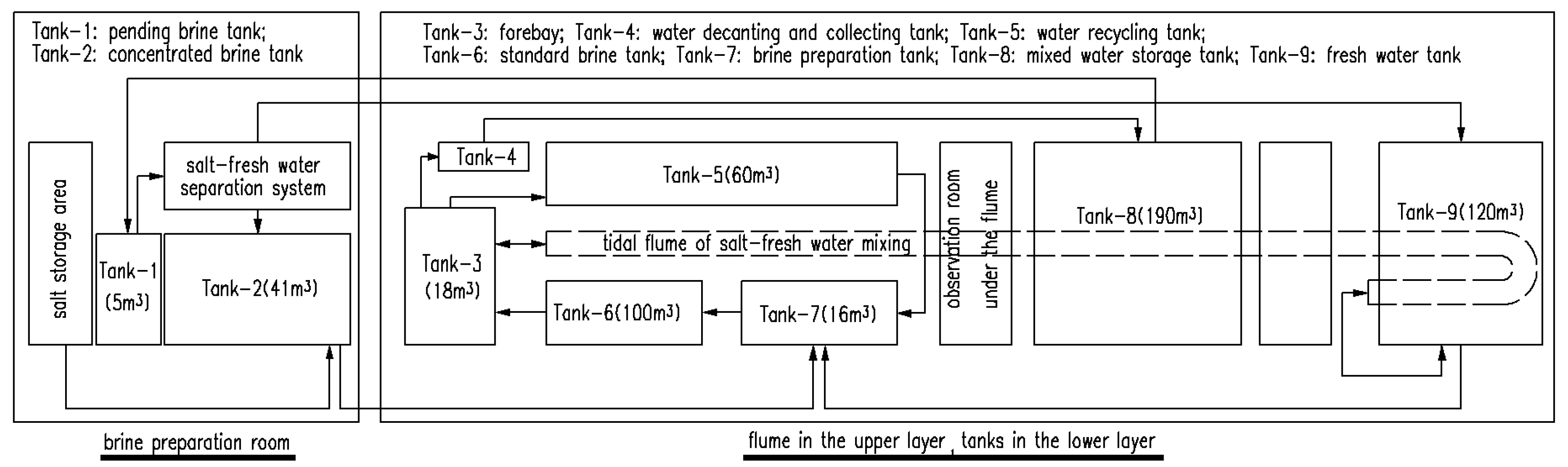
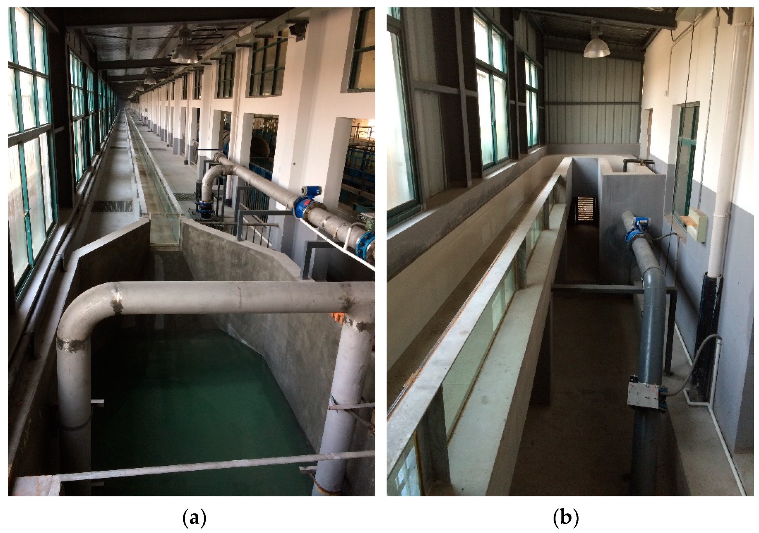
2.1. Flume Layout and Brine Treatment

The flume has a total length of 167.8 m, a net width of 0.5 m and a depth of 0.5 m (Figure 1). Its length is greater than the saltwater intrusion length in the flume, so that the downstream salt water will not be mixed into the upstream freshwater tank. Its depth meets the needs of the tidal level change and the full development of salt-fresh water mixing.

Downstream layout of the flume: The downstream end of the flume was connected to the forebay supplying the tidewater and brine (Figure 2a). A tail gate was provided at the exit of the forebay. The tidal level was remotely and accurately controlled by the tail gate of flap type combined with the wireless measurement and control technology. The tail gate was driven by an variable frequency controlled inverter AC motor, and the absolute error between the actual water level and the set value was reduced to less than 1 mm on average.

Upstream layout of the flume: The upstream end of the flume was connected to a reversible pump, and the tidal current discharge was controlled by an electromagnetic flowmeter (Figure 2b). The reversible pump controlled the upstream boundary discharge, and combined with the tidal level control at the downstream boundary, the reversing flow velocity in the flume reached up to about 20 cm/s. In addition, the fresh water inlet pipe set at the upstream simulated the discharge of runoff through the flow meter, and the runoff reached up to 12 m³/h.

Layout of reservoirs: The test consumed a large amount of water, the water quality was complex, and the salinity control requirement was high. The process of mixing, conveying, circulation and recycling of salt-fresh water was shown in the figure. The reservoirs consisted of a standard brine tank, a forebay, a water decanting and collecting tank, a brine preparation tank, a water recycling tank, a mixed water storage tank, a concentrated brine tank, a pending brine tank, and a fresh water tank. The tanks were independent of and were also connected to one another through the submersible pump, which enhanced the test accuracy and efficiency.

Preparation of brine: The preparation of the test brine was carried out in several tanks: ① the brine with big concentration was prepared in the concentrated brine tank; ② the concentrated brine was pumped into the brine preparation tank, and freshwater was added to prepare the standard brine for the test as per the required salinity; ③ the brine reaching the standard was pumped into the standard brine tank for the test; ④ the diluted brine discharged during the test entered the brine preparation tank through the water recycling tank, and it would be pumped into the standard brine tank after being re-prepared and meeting the standard.

Recovery of mixed water after the test: ① After the test, the brine in the standard brine tank, forebay and water recycling tank was pumped into the mixed water storage tank by the submersible pump; ② the brine in the mixed water storage tank was pumped into the pending brine tank; ③ the brine was pumped out of the pending brine tank through the salt-fresh water separation system, and the freshwater reaching the standard after filtration and separation was pumped into the fresh water tank, and the concentrated brine into the concentrated brine tank.

2.2. Data Acquisition

The input conditions of the test were mainly the tidal level hydrograph and discharge hydrograph. The control system automatically controlled the water level and flow according to the given conditions and the main measurement interval of the test data was 0~140 m from the mouth (entrance of the glass flume segment). The section after 140 m was completely occupied by the upstream freshwater, which did not fall within the scope of the study.

2.2.1. Flow Velocity Data Acquisition

One-dimensional flow velocity: 24 photoelectric propeller-type current meters were used and 6 were set on each section to measure the flow velocity on four sections simultaneously; the meters were set at an interval of 10 m from 0 to 140 m on the gauging section (the section numbers were the distance from the downstream starting point of the flume); the measuring point of each section was arranged using the six-point method, namely, current measurement at surface, 0.2h (h means water depth, the same below), 0.4h, 0.6h, 0.8h and bottom. The propeller type current meter was suitable for measuring one-dimensional average flow velocity. The average flow velocity values were collected every 4 s in the test.

Two-dimensional and three-dimensional flow velocity: The instruments were FlowTracker ADV two-dimensional current meter and Vectrino three-dimensional current meter. The two meters coordinated each other and mainly measured longitudinal and vertical flow rate. They were set at an interval of 10 m from 0 to 140 m on the gauging section and measured the current on the surface, middle and bottom layers of each section. With regard to the current measurement at the salt-fresh water interface, Vectrino current meter was used for tracking measurement for the purpose of data acquisition of the vertical fluctuating velocity at the interface.

2.2.2. Salinity Data Acquisition

Sampling and salinity measurement: The instruments were self-made sampling device and conductivity meter. The instruments were set at an interval of 10 m from 0 to 120 m on the salinity measurement section. The six-point method was adopted for section sampling, namely, salinity measurement at surface, 0.2h, 0.4h, 0.6h, 0.8h and bottom. Water samples were taken every 1 min. The brine was mainly distributed at the bottom after 120 m and the conductivity was measured manually using a hand-held conductivity meter. After the test, the conductivity of all samples were measured and converted to salinity. The conversion relation was actually measured according to the various ratios of the test fresh water and the industrial salt (sodium chloride content >99%). The salinity refers to the number of grams of dissolved matter in 1000 g solution, which is a dimensionless number.

Synchronous salinity and velocity measurement using ADV current meter: The test arranged the conductivity meter and the Vectrino current meter probe at the same depth and kept a certain distance between them. The current measurement and salinity measurement were conducted simultaneously.

Salty boundary position measurement: The position with bottom salinity of 0.25 was taken as the salty boundary (or the saltwater wedge tip) position, which generally moved in a certain range with the flood and ebb tides. During the measurement, a hand-held conductivity meter was used to track the movement of salty boundary in a real-time manner. The position of salty boundary was recorded once every minute, the maximum and minimum upstream movement distances of salty boundary were measured, and the positions of salty boundary at the time of flood slack and ebb slack were recorded.

2.2.3. Other Data Acquisition

Water level data acquisition: Two fixed water level gauges automatically recorded the water level changes at 0 m and 55 m respectively, automatically entered the data into the computer and recorded the water level once every second; a movable water level gauge recorded the water level changes at 30 m, 90 m, 120 m and 140 m and recorded the water level once every 15 s.

Saltwater wedge height: In the highly stratified type of salt-fresh water mixing, brine often intruded freshwater in the form of saltwater wedge. Some rulers were attached to the outer wall of the flume to record the height changes of the wedge at 10 m, 30 m, 50 m, and 70 m, and the data was manually recorded once every 30 s.

Video recording: The side wall of the flume was made of transparent glass to facilitate the observation of test phenomenon. A 4 m-long observation chamber was provided at 50 m and 106 m respectively from the head of the flume. The observation chamber was under the flume, the bottom of which was made of glass, when the other flume bottoms were made of ceramic tiles. The test used a high-definition video camera to record the full cycle of the salt-fresh water mixing process at 10 m, 30 m, 50 m, 70 m, 110 m, and a SLR camera to shoot the test phenomenon.

2.3. Test Repeatability

To guarantee the cycle repeatability of salinity and velocity data, before data acquisition, it was necessary to wait for the salt-fresh mixing to reach the quasi-steady state, and the salty boundary movement range to change periodically. In the test, the carmine pigment was added to the brine to facilitate visual observation. Through the detection of conductivity meter, the carmine pigment had little effect on the conductivity of brine and did not affect the determination of salinity. The preliminary test results showed that after more than 5 tidal cycles, the salt-fresh water mixing reached the quasi-steady state, and data acquisition after that provided good cycle repeatability.

The repeatability test mainly included the following contents:

• Velocity repeatability test: 12 min was taken as a tidal cycle and the velocity repeatability under the conditions of several cycles on the same day, the same input conditions on different dates and different flow measurement equipment at the same measuring points were verified.
• Buoy displacement test: A buoy was placed on the water surface at a certain interval to record the limit position that the buoy reached in each tidal cycle. The results showed that the drift range of the buoy tended to be stable.
• Salty boundary repeatability test: The position of the salt boundary was recorded at set intervals. The results showed that the change of the salt boundary at the quasi-steady state tended to be within a certain range.
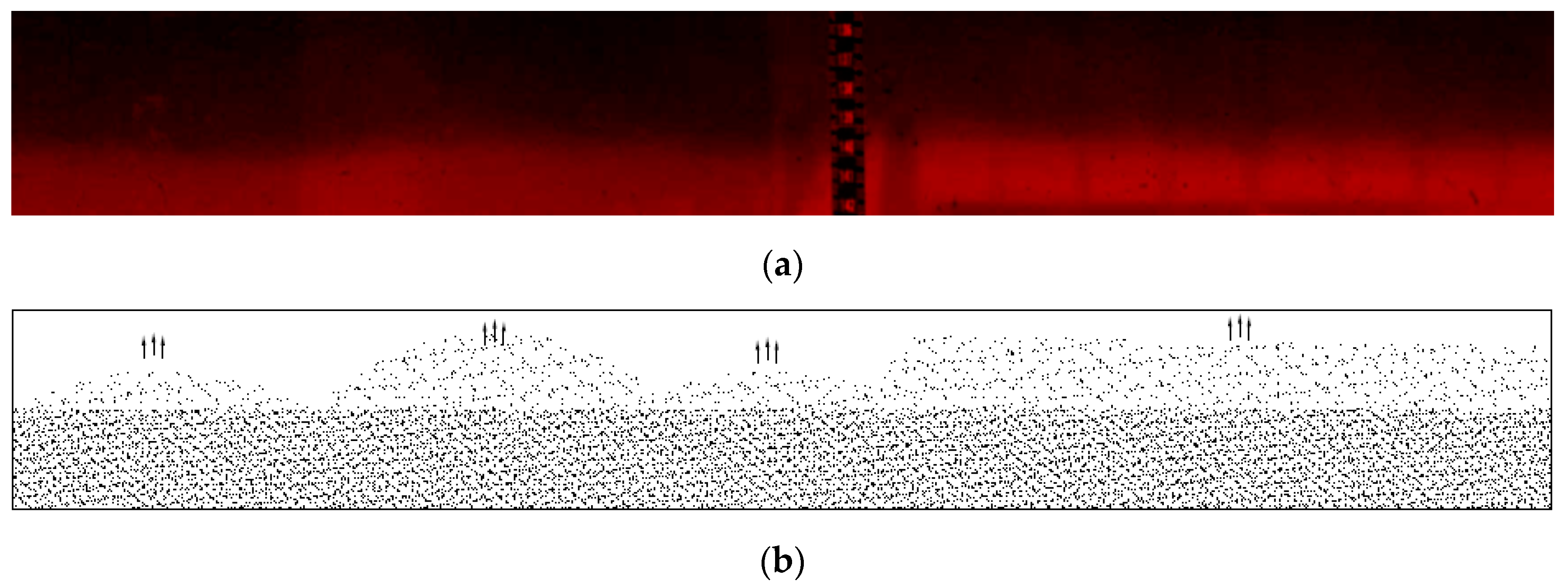
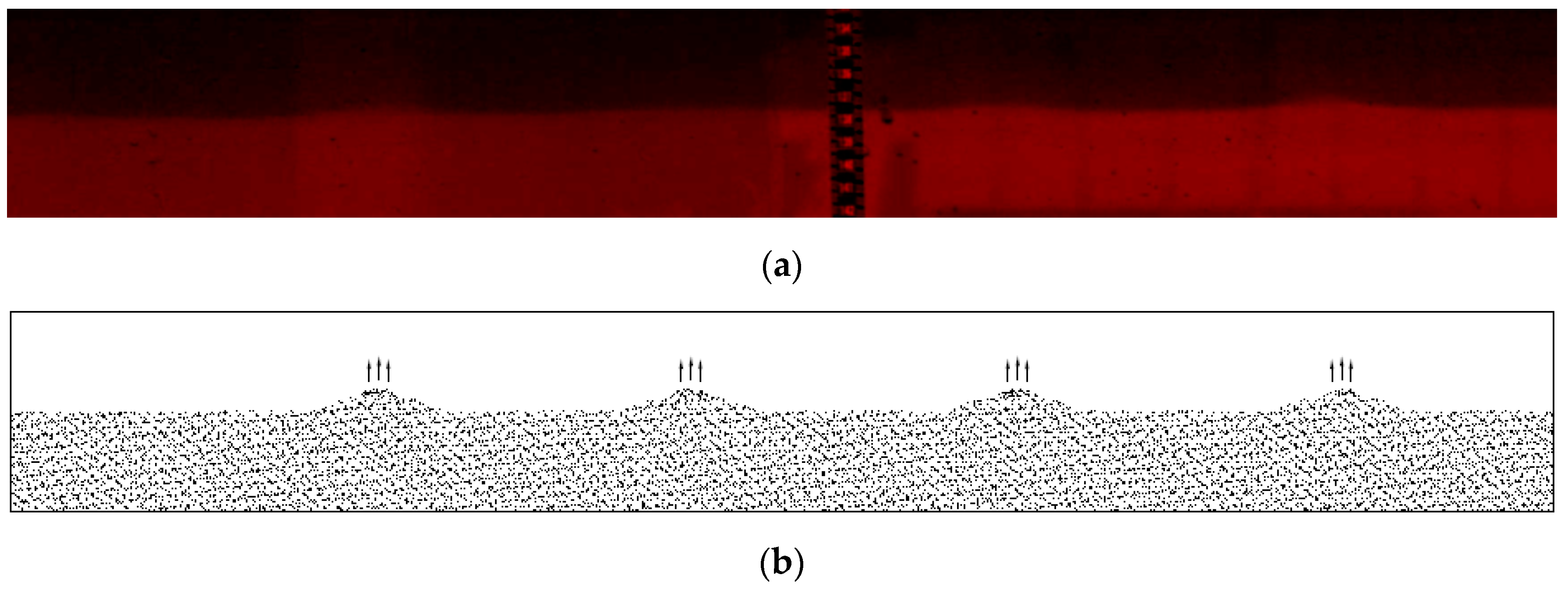
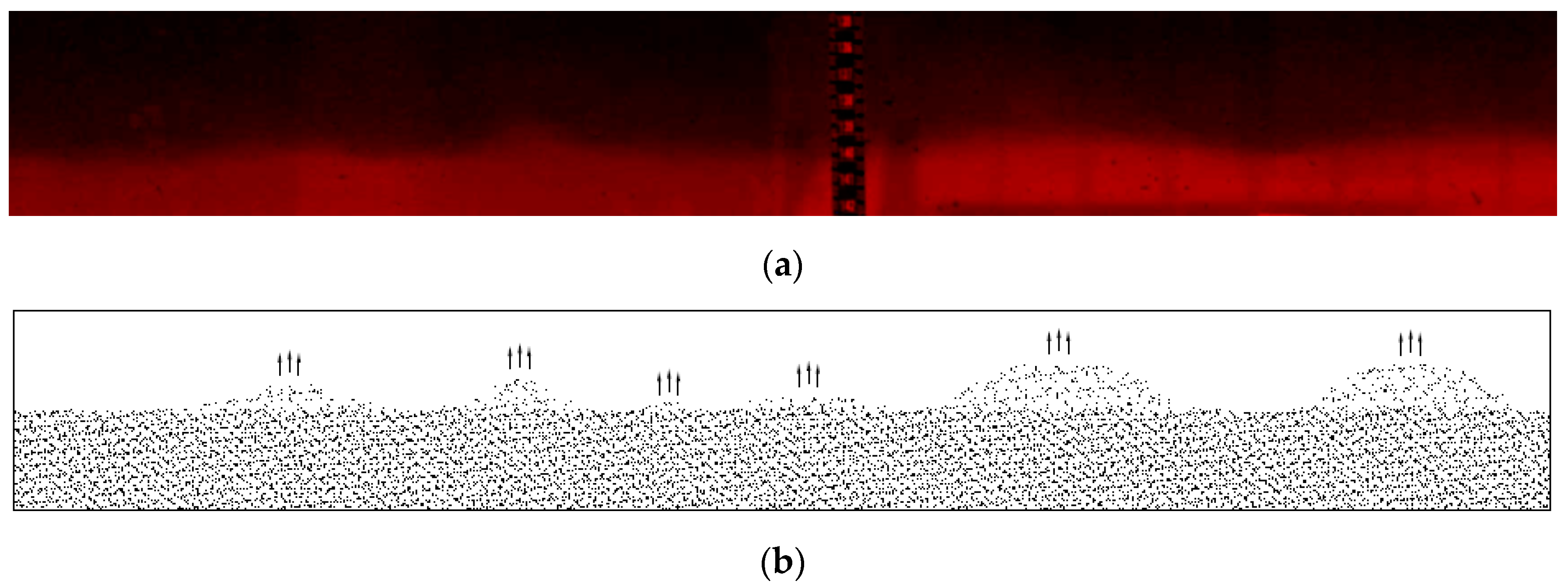
• Wedge thickness repeatability: Near the upstream, the brine intruded in a wedge shape. The video records showed that the wedge thickness and water depth at any time were almost constant after a tidal cycle.
• Salinity repeatability: The salinity of the same section in each layer was measured for two consecutive cycles. The repeatability of both the salinity of each layer and the depth averaged salinity must meet the test requirements.

2.4. Test Conditions

The estuarine salt-fresh water mixing was subject to dynamic changes due to the impact of dynamic and water depth conditions. To study the influence of tide, runoff and water depth on salt-fresh water mixing, the control variable method was applied to the flume test.

Salinity conditions: An actual estuary was required for the implementation of flume test simulation, and the salinity conditions were designed as per the ratio of 1:1. As the test flume was straight and gentle, and in order to study the variation characteristics of the salt-fresh water interface with the tide, the middle and upstream reaches of the North Passage of the Yangtze River estuary were selected as the prototype segment and the saline intrusion front was basically located in this segment. According to the hydrological data in 2012 [32], the salinity of the South Channel and Yuanyuansha reach was basically below 3, and that of the upstream reach of the North Passage was between 3 and 7, while that of the middle and downstream reach of the North Passage was basically in the range of 7~12. Accordingly, the initial condition of salinity in the flume test was set to about 10, and the preparation of brine was carried out according to the average salinity in the forebay of the flume.

Tidal conditions: To study the influence of tide strength changes on salt-fresh water mixing, four model tidal ranges of 4 cm, 3 cm, 2 cm and 0 cm were selected to simulate the water flow movement under the conditions of spring tide, moderate tide, neap tide and tideless situation, the tidal level hydrograph was sine curve and the tidal cycle was set to 12 min. The upstream segment of CSW survey point in the North Passage was taken as the prototype. It was assumed that the length scale of the prototype and the model was 750, the height scale 150, and the flow velocity scale 12.25. The maximum flow velocity of the North Passage reached up to about 2.5 m/s and the maximum flow velocity in the flume should reach 20 cm/s as calculated as per the velocity scale. After debugging, the maximum flow velocity in the flume reached up to 20~25 cm/s during spring tide and 10~15 cm/s during neap tide, which were in line with the test requirements.

Runoff conditions: To study the influence of runoff intensity changes on salt-fresh water mixing, and to simulate the partially mixed type and highly stratified type, the test set runoff through the calculation of the ratio of runoff to tidal discharge [33]. The partially mixed type corresponded to a ratio of about 0.2~0.5 and the required runoff was calculated after combination with the flood tidal volume in the flume, and it was set accordingly by the flow meter at the upstream end of the flume. By virtue of calculation and previous test experience, the runoff was set to 0 (no runoff), 3 m³/h (mainly simulating partially mixed type), 6 m³/h and 11 m³/h (simulating highly stratified type) to satisfy different test requirements.

3. Results

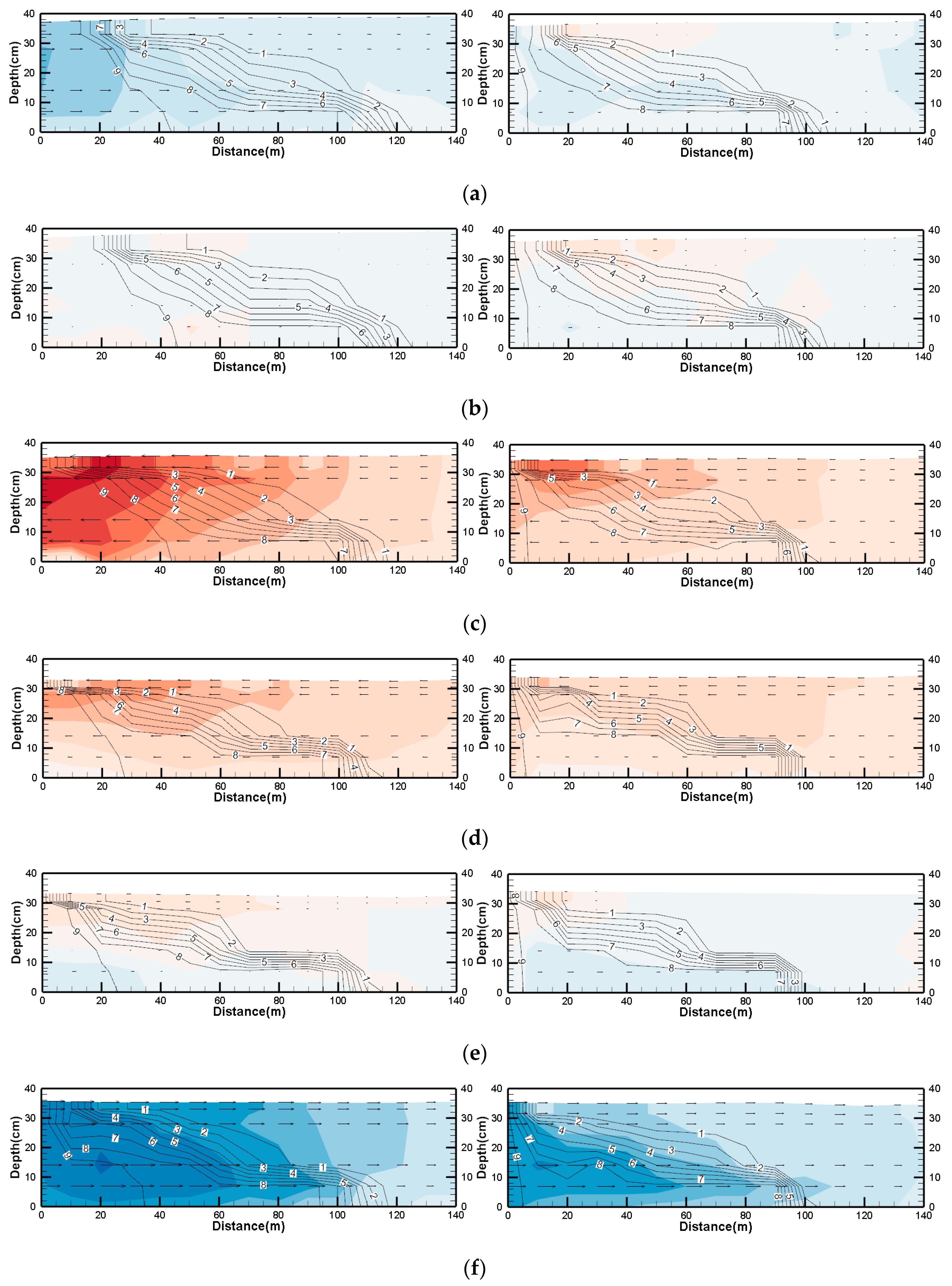
3.1. Influence of Tidal Range on the Mixed Type of Salt-Fresh Water

In the test, the influence of tide intensity changes on the mixed type of salt-fresh water was studied by changing the tidal range. Taking Case 1 and Case 2 as examples (working conditions were shown in

Table 1. The conditions of Case 1 and Case 2.

Case	Tidal Range (cm)	Runoff (m3/h)	Average Depth (cm)	Initial Salinity	Water Temperature (°C)
1	4	3	35	10.1	9.9
2	2	3	35	9.5	9.7

), the salinity distribution was roughly divided into three segments on the whole (Figure 3). The first segment with obvious characteristics of fully mixed type was roughly distributed in the near-mouth reach (0~10 m). The salinity contour of this segment tended to be vertical, especially evident during maximum flood to flood slack. The second segment with obvious characteristics of partially mixed type was basically distributed in the middle and downstream reach (10~70 m). The salt-fresh water in this segment was partially mixed, which was also the main mixed type of the partially mixed estuary. The salinity contour was generally inclined and the salinity gradually increased from the surface layer to the bottom layer. The third segment characterized by highly stratified mixed type was generally distributed in the upstream reach (after 80 m). This segment had obvious salt-fresh water stratification. Its salinity contour was approximately horizontal, and the brine intruded in a wedge shape. The distribution range of these three segments varied greatly with the flood and ebb tide, but was consistent in terms of the order.

Simpson et al. [34] proposed the potential energy anomaly at a rather early stage, introduced the concepts of tidal straining and tidal stirring, and further studied the effect of tidal action on estuarine salt-fresh water mixing. In the test, from the perspective of the high water, the fully mixed segment of spring tide was significantly longer, indicating more apparent tidal stirring. Without such tidal stirring, the brine would intrude along the bottom in the form of density current, which has been confirmed in many previous saltwater wedge tests. The tidal stirring exactly played the role of transporting the bottom salt to the upper layer, and the greater the tidal strength, the more apparent the tidal stirring, thus resulting in the thorough mixing of salt-fresh water. As the Qiantang River estuary is a macrotidal estuary, its fully mixed type is inseparable from the tidal stirring.

As shown in Figure 3, the effect of tidal stirring was more obvious during the flood tide period. After flood slack tide, under the joint action of runoff and ebb current, the salt and freshwater were transported downstream, leading to the decrease of surface salinity, the downstream inclination of contour with the salinity of 1 and the transition of fully mixed type to partially mixed type. This situation was different at the time of spring and neap tides. The fully mixed area covered by the contour with the salinity of 9 during spring tide was larger than that during neap tide, which was mainly because of the differences on tidal stirring and flow turbulence. In general, the fully mixed effect during spring tide was stronger, and the neap tide was conducive to partially mixed effect and stratified flow development.

Theoretically speaking, the salinity dispersive transmission caused by tidal straining will result in inhomogeneous distribution of salinity in the vertical direction, thus inhibiting the formation of fully mixing, which is contrary to the effect of tidal stirring. How to evaluate the relationship between the two contradictory actions (tidal straining and stirring) is an important aspect in the study of the impact of tidal strength on salt-fresh water mixing.

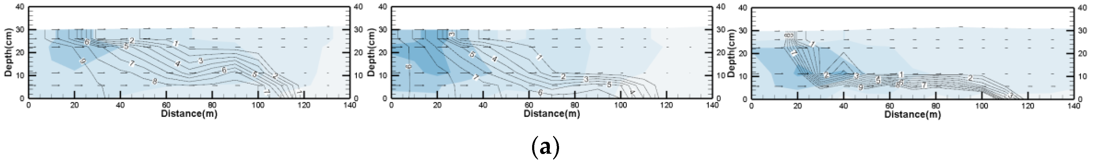
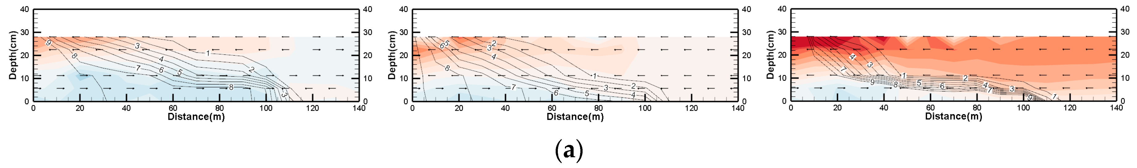
3.2. Influence of Runoff on the Mixed Type of Salt-Fresh Water

The role of runoff is mainly to superimpose a downstream freshwater flow upon the original hydrodynamic conditions of the estuary, which increases the downward salt flux, and thus inevitably leads to a decline in the overall salinity of the estuary.

Taking Case 3 and Case 4 as examples (the runoff increased in turn, as shown in

Table 2. The conditions of Case 3, Case 4 and Case 5.

Case	Tidal Range (cm)	Runoff (m3/h)	Average Depth (cm)	Initial Salinity	Water Temperature (°C)
3	4	0	28	10.1	10.4
4	4	3	28	9.4	9.6
5	4	11	28	18.8	10.8

), judging from the high water and flood slack moments, the salinity contour in the upstream reach of 50 m section gradually sloped more gently as the runoff increased due to the blocking effect of the runoff (Figure 4). During the ebb tide period, the surface velocity increased significantly as the runoff increased, the salinity contour was concentrated towards the flume entrance, and the salty boundary was retreated to the downstream. At the maximum ebb tide, the salinity contour was inclined to the bottom as the runoff increased. At the ebb slack tide, the partially mixed segment gradually shrank and transitioned to the highly stratified type as the runoff increased. The impact of runoff on the tidal current was reflected in the increase of ebb velocity and weakening of flood current, as indicated at the moments of maximum ebb and maximum flood tide.

Unlike Case 3 and Case 4, Case 5 significantly increased the initial salinity and runoff, aiming to simulate the mixing type of saltwater wedge (Figure 4). In Case 5, the salinity contour was almost horizontal under the strong runoff condition, the salinity was basically unchanged along the bottom, and the mixing type of saltwater wedge became a dominant type. At the maximum ebb tide, the wedge surface was unstable under the entrainment effect, the salt water was vertically mixed into the upper fresh water, and the contour with the salinity of 1 had local bulging.

Therefore, the main effect of runoff with certain intensity on salt-fresh water mixing was to continuously strengthen stratification and weaken mixing, and even change the mixing type of the estuary during a sudden flood. However, the vertical mixing emerging on the saltwater wedge surface at the maximum ebb tide appeared to complicate the simple proportional relation between runoff intensity and stratification.

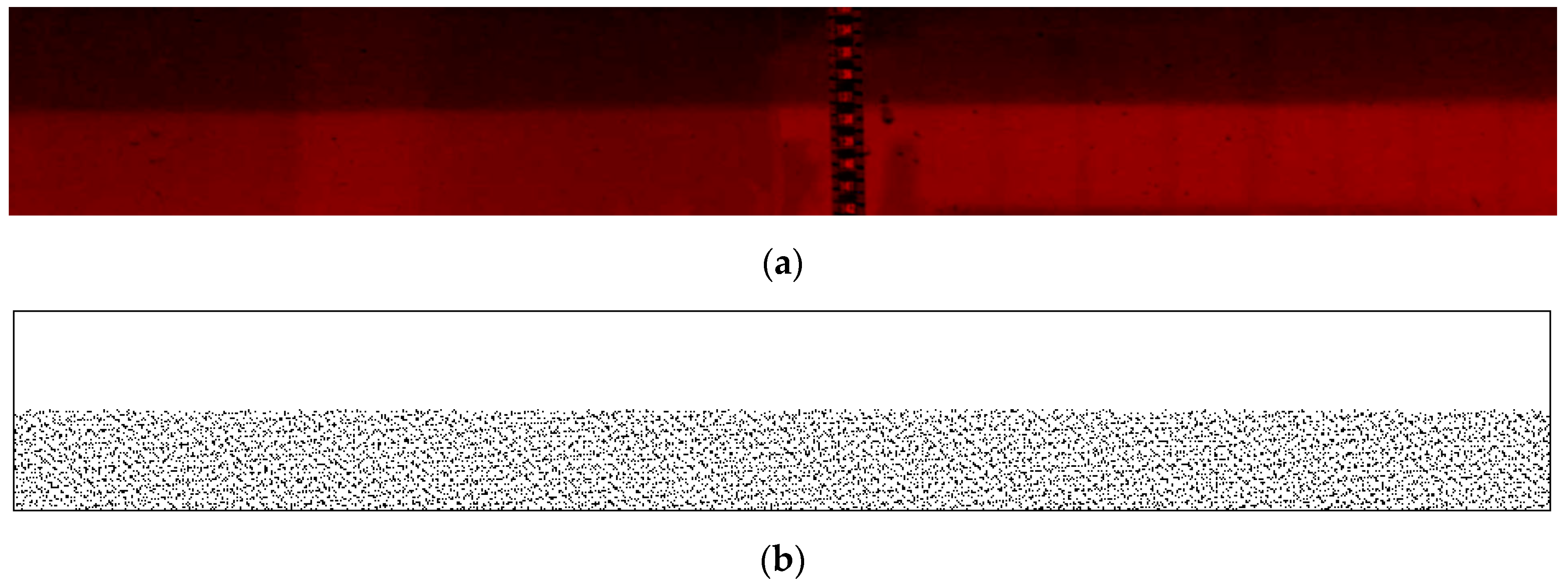
3.3. Change of Salt-Fresh Water Interface in the Condition of Tidal Reciprocating Flow

In this flume test, the water stratification phenomenon was particularly apparent in the middle and upstream reaches and during the ebb tide period, characterized by a relatively clear interface between salt water and freshwater. To observe the mixed state of salt-fresh water, the carmine pigment was added to the brine. Through the detection of conductivity meter, the carmine pigment had little effect on the conductivity of salt water and did not affect the determination of salinity.

In Case 5, the upstream water in the flume showed a saltwater wedge type. At the moment of high water, the interface was still smooth and clear (Figure 5). However, after the start of flood tide, the internal waves appeared on the interface in the propagation form of solitary waves distributed at intervals. As the flow velocity increased, the interface gradually showed K-H instability, and the wave peak started to break, manifested by the diffusion of a small amount of colored water into the upper colorless water (Figure 6). The wavelength decreased with the increase of the flow velocity, and the number of wave peaks per unit length increased. At the moment of maximum ebb tide, the flocculent colored water generally appeared above the interface, and was transported downstream with the ebb current (Figure 7 and Figure 8). After the ebb current velocity decreased, the wave peak gradually became lower and widened. At the ebb slack water, it was seen that standing waves appeared at the interface, which should be caused by the superposition of the inertial flow of the ebb and the tidal wave from the downstream. During flood tide, the change of internal waves was similar to that during ebb tide, the difference was that the fluctuation scale during flood tide was bigger, and the interface fluctuated as affected by the tidal wave.

4. Discussion

4.1. Improvement of Flume Test Technology

Due to the generalization of the flume test, the model size should be designed according to the research objective. Regarding the measurement technology in the test, it is necessary to carry out full-scale observations for the velocity field, salinity field and water level changes. In the aspect of test operation, it is necessary to accurately control the flow velocity, water level, etc. For the experimental water, it must be treated in strict accordance with the environmental protection requirements, and the recycling, desalination and reserve of brine are the key issues to be solved. In this flume test, improvements and innovations have been made in the following aspects.

The salt-fresh water mixing under the tidal reciprocating flow was successfully reproduced: the salt-fresh water mixing and stratification changes of the estuary under the tidal reciprocating flow conditions were simulated through the tide and runoff control systems at both ends of the flume, and the reciprocating current velocity in the flume could reach 20 cm/s. The tidal level was remotely and accurately controlled by a tail gate of flap type combined with wireless measurement and control technology, and the tail gate was driven by a variable frequency controlled inverter AC motor. The upstream end of the flume was connected to a reversible pump combined with an electromagnetic flowmeter to control the tidal discharge. It could realize complete closed-loop control with small error and good test repeatability. This was especially important for tests requiring long-term uninterrupted operation.

In order to truly reflect the reciprocating flow characteristics of the tidal current and the periodic changes of the water level, the test operation has met the following requirements after equipment debugging and energy dissipation measures: ① Under the condition of no runoff, the net tidal volume passing through a section in a tidal cycle was approximate to 0; ② the flow reverberation and abnormal tide level fluctuations caused by tidal wave reflection were attenuated to reduce the test error; ③ the measured tidal level and discharge hydrograph of the model fit well with the set value, without abnormal large-scale fluctuation.

The length of the straight segment of the flume was improved and the research scope of the current flume test expanded: In the previous experimental study of salt-fresh water mixing, the length of the flume often limited the scope and depth of study. For example, the short flume [35] limited the scope of research. The length of the flume should be greater than the saltwater intrusion length, so as to prevent the downstream brine entering the upstream freshwater tank. The depth needs to meet the needs of the tidal level change and the full development of salt-fresh water mixing. In the flume test of the Pearl River Hydraulic Research Institute [28], the maximum length of saltwater intrusion without tide exceeded 100 m, and the maximum length of saltwater intrusion reached up to 88.6 m during flood tide when the tidal range was 1 cm. With reference to the existing documents, the new test flume built in the research had a total length of 167.8 m (straight length of 160 m), a net width of 0.5 m and a depth of 0.5 m. The flume size has fully satisfied the research needs of salt-fresh water mixing and expanded the scope of research.

The initial salinity was maintained by surface diluted water decanting technology: the upstream freshwater was easily mixed into the downstream forebay during the test, leading to the decrease of initial salinity in the pool and the difficulty in maintaining the constancy of initial salinity, thus resulting in experimental error. The self-designed decanting device used in the research was able to automatically decant the surface diluted water during ebb tide and prevent diluted water from entering the forebay substantially. In this way, the frequency of initial salinity regulation was reduced, work efficiency enhanced, and the difficulty in controlling the initial salinity of the open sea boundary of the model overcome.

Recycling the test wastewater to eliminate pollutant emission: The sluice boards were provided at 0 m, 30 m, 60 m, 86 m and 112 m respectively from the flume entrance to cut off the fluid in the flume. After the test, the sluice boards were closed to separate water with different salinity and divert it into different tanks for saltwater treatment. The membrane separation technology was used to desalinate and separate the mixed water, and the concentrated brine and freshwater were separately stored for the next use to achieve zero discharge of the test wastewater.

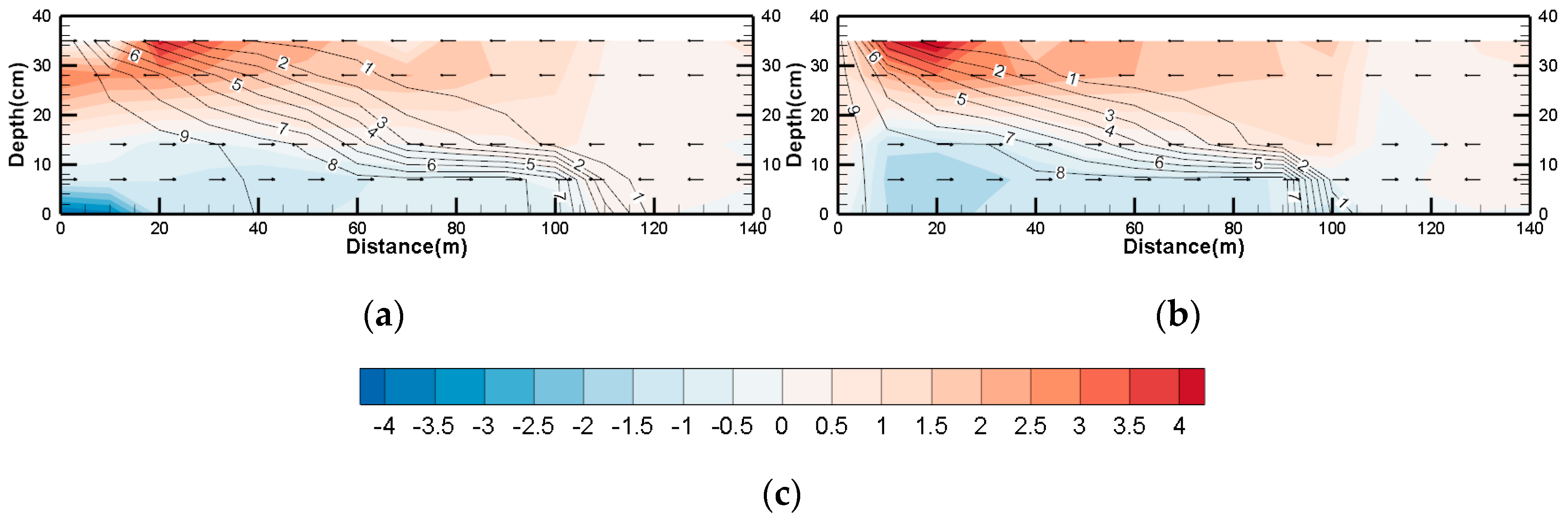
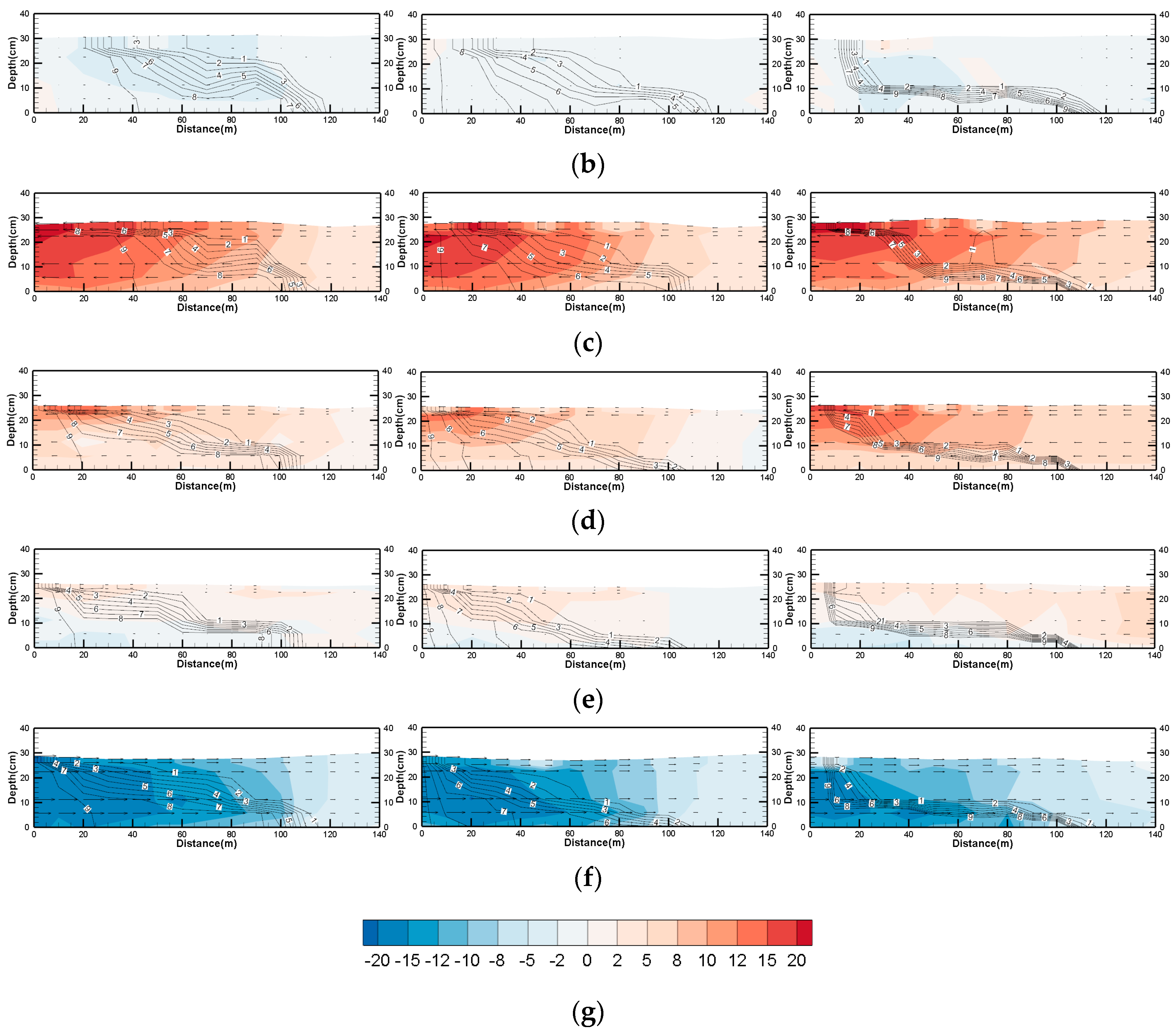
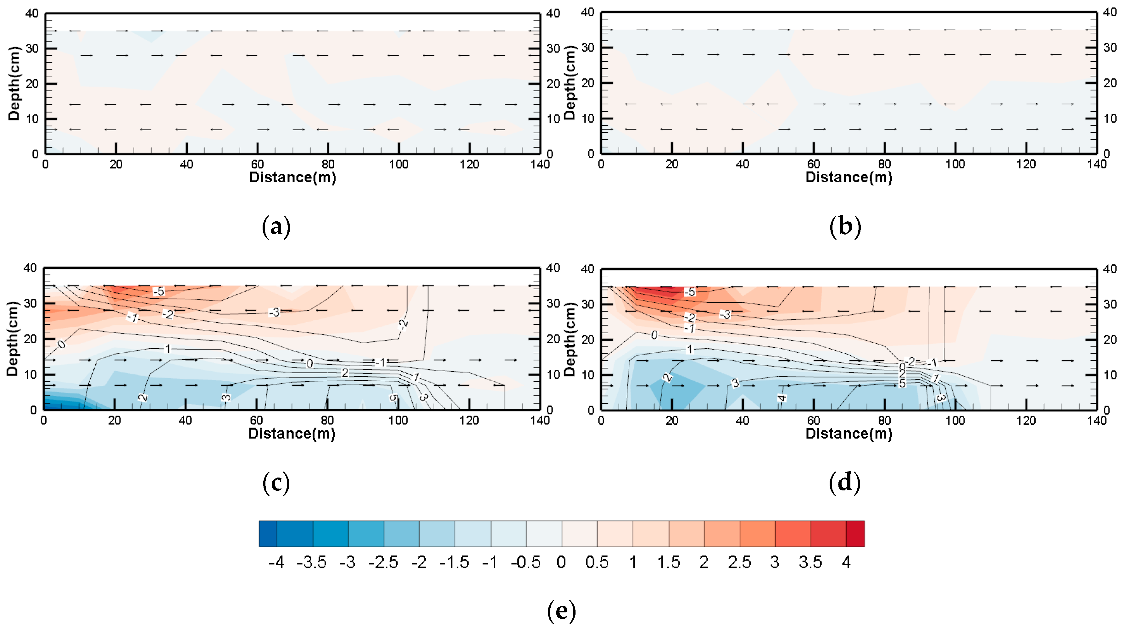
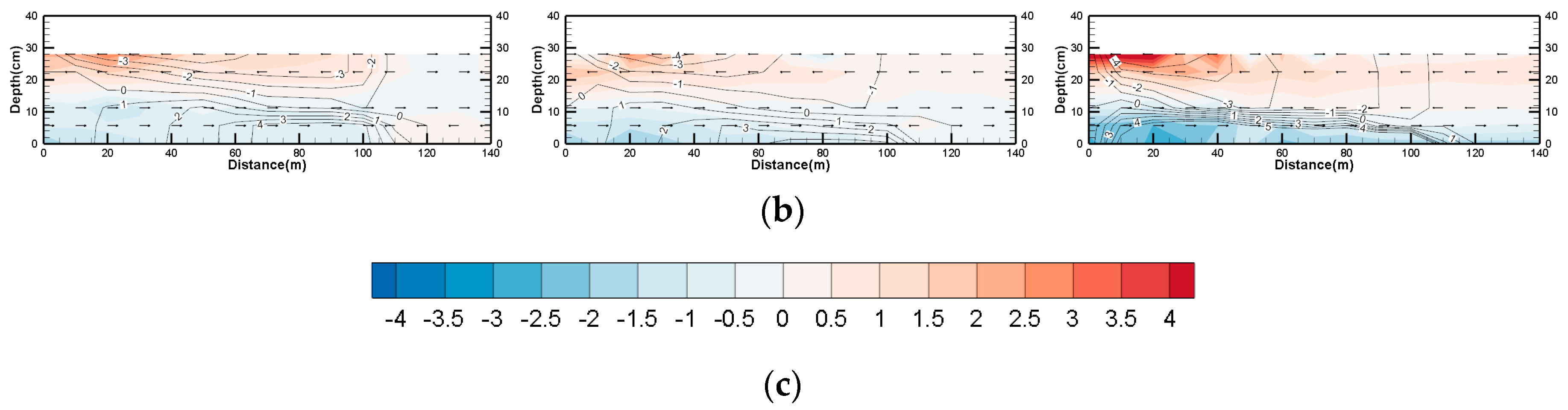
4.2. Characteristics of Gravitational Circulation and Residual Circulation

In the actual estuary, the change of salt-fresh water mixing with the dynamic process is very complicated. The research is mostly based on the “quasi-steady state”, that is, on the state averaged over a tidal cycle. Unlike the velocity distribution of freshwater rivers, the flow structure formed by the salt-fresh water mixing in the tidal estuary often has the characteristics of residual circulation and gravitational circulation. That is to say, the lighter fresh water flows downstream in the upper layer, when the heavier salt water flows upstream in the lower layer. The circulation has great influence on salinity distribution, and the salt-fresh water stratification also leads to the change of circulation structure. It was considered that the vertical circulation was generated by the interaction between the water surface gradient and the horizontal density gradient [19,36]. Through studying the influence of water density changes on the flow, it was believed that the estuarine circulation was driven by the pressure gradient force [37]. The adjustment of estuarine circulation to changes in river flow and tidal mixing was investigated using analytical and numerical models [38]. According to the results of the flume test in this paper, the circulation characteristics under the changes of tidal range and runoff can be analyzed, so as to study the dynamic mechanism of salt-fresh water mixing and stratification under the steady state.

4.2.1. Circulation Characteristics under Tidal Range Change

The velocity of residual circulation was calculated by the following formula, which was averaged over a tidal cycle.

$$\overline{u}=\frac{1}{T}{\displaystyle {\int }_0^{T}udt,}$$

(1)

where T is the time of flood and ebb cycle; u is the longitudinal velocity; the overbar denotes the average over a tidal cycle.

The velocity of gravitational circulation is the residual current velocity at one point minus the residual current velocity averaged over the depth, as follows.

$${\overline{u}}_G=\overline{u}-\frac{1}{h}{\displaystyle {\int }_0^h\overline{u}dz,}$$

(2)

where h is the water depth; ${\overline{u}}_G$ is the velocity of gravitational circulation.

As indicated by Figure 9, the residual circulation form was manifested as that the diluted water in the surface layer was transported towards the downstream, while the concentrated brine at the bottom moved upstream. The change in the tide strength caused a slight change in the residual current field. On the near-entrance section, the residual current velocity at the bottom in spring tide was bigger, demonstrating that a stronger tidal action enhanced the net inflow at the bottom; while the surface velocity in neap tide was higher, demonstrating that relatively enhanced runoff increased the net outflow in the surface layer. From the point of view of salinity distribution, the enhanced tidal effect during spring tide increased the horizontal salt transport of tidal current, and the saltwater intrusion length was longer than that during neap tide. The analysis of the residual current field included the net transport of runoff to the downstream, which can be calculated by averaging over the depth and a tidal cycle. If the residual current velocity at one point minus the residual current velocity averaged over the depth (Equation (2)), the velocity of gravitational circulation can be got and the profile figures of gravitational circulation were shown in Figure 10.

The gravitational circulation was mainly caused by the baroclinic effect of density gradient. Equations (1) and (2) showed that the residual circulation and the gravitational circulation differed by the depth-averaged residual current and it should be zero if the gravitational circulation velocity in vertical was integrated along the water depth. The same method as the calculation of gravitational circulation was used to calculate the salinity, to reflect the distribution rule of the time-averaged salinity in the vertical direction. The comparison between saltwater condition and freshwater condition stated clearly the change of the gravitational circulation current field before and after salt addition. After the addition of salt, several physical quantities were added or increased, the first was density gradient, the second was water mass, and the third was buoyancy. Assuming that the influence of external factors (tide, runoff, etc.) was not taken into account, the horizontal density gradient force generated by the density difference caused the fluid to flow from the high density zone to the low density zone in the horizontal direction, and enhanced the molecular diffusion effect at the fluid interface; the increased mixed water mass enhanced the effect of the inertial force; the buoyancy generated by the high-density water body to the low-density water body kept the low-density water body moving at the upper layer. Under the combined actions of these forces, the gravitational circulation structure was formed. Many past documents pointed out that gravitational circulation had the effect of intensifying stratification, and that the estuary with the bigger depth was more conducive to the formation of gravitational circulation. This test showed that the increase of tidal strength weakened the gravitational circulation near the entrance, but appeared to have an insignificant impact on the gravitational circulation structure in the middle and upper reaches. The enhanced tidal stirring caused the upstream movement of salinity difference -5 in the surface layer for a short distance, without big changes in the vertical difference of cycle-averaged salinity at each layer, demonstrating a limited impact of tidal stirring on the distribution of salinity at a steady state in the vertical direction.

4.2.2. Circulation Characteristics under Runoff Change

As indicated by the comparison of residual current fields under different runoff conditions (Figure 11), with the increase of runoff intensity, the net outflow of the surface layer was enhanced and the closer to the entrance, the bigger the flow velocity was; the lower and middle reaches of the bottom layer were manifested as net inflow and a gradually reduced range; the upper reach of the bottom layer was manifested as net outflow and a gradually increased range. There were various indications that the runoff added a net downstream freshwater flow to the estuarine water, thus changing the salinity field. As the runoff increased, the upper and middle reaches of salinity contour sloped more gently, suggesting the gradual transition of the salt-fresh water mixing structure to the saltwater wedge, and obvious stratification; the downstream salinity contour became steep, and the partially mixed type was obvious.

From the perspective of gravitational circulation, the larger runoff and initial salinity of Case 5 remarkably increased the intensity of gravitational circulation and the longitudinal density gradient near the entrance was larger than that of Case 3 and Case 4, demonstrating that the gravitational circulation intensity was positively correlated to the runoff and the longitudinal density gradient. From the perspective of the distribution of salinity difference contour, as the runoff intensity increased, the pycnocline tended to gather towards the bottom and it was distributed near the wedge surface in Case 5, which reflected the compression of runoff on the estuarine salinity field, and such compression strengthened the stratification of salt-fresh water.

According to the above analysis, the results vary when the effect of runoff on salt-fresh water mixing is seen from different time scales. From the point of view of the tidal cycle-averaged steady state, the runoff induced the gravitational circulation of the estuary and was able to strengthen this effect. The bottom salt was continuously replenished and entered the upper layer through turbulent diffusion. The salt of the upper layer was continuously lost with the diluted water moving downstream, thus forming a dynamically balanced salinity field. The superposition of the salinity field caused by the gravitational circulation on the steady-state field always played a role of stabilizing stratification.

However, from the perspective of the dynamic process, the effect of runoff on salt-fresh water mixing was the same as that of tide and there were also two seemingly contradictory dynamic mechanisms. The balance between these two mechanisms was the balance between vertical density gradient and velocity shear, as well as the balance between longitudinal convective transport and vertical diffusion. The former was from the perspective of dynamic balance, while the latter was evaluated from the perspective of conservation of mass. The increase of runoff could maintain the vertical density gradient of the salt-fresh water interface--stabilizing stratification, and increase the velocity shear of the interface as well--destroying stratification; could export the salt by the convective flow-- stabilizing stratification, and extract the diffused salt from the lower layer through the perturbed interface as well--destroying the stratification. However, this process was far more complicated than described here, and it was analyzed only from the vertical two-dimensional perspective in this paper.

4.3. Analysis of Salt-fresh Water Interface Stability

For highly stratified fluid motion, the interface stability is always a research hotspot. The interfacial internal waves and instability were mostly studied from the perspective of the increase or attenuation of small disturbances previously. Kelvin and Helmholtz have studied the interface stability earlier. The interfacial instability and mixing of stratified flows were studied through the flume test of saline wedge [13]. In addition, an experimental study was made on the entrainment of stratified flow interface [39]. Citing the laboratory experiments performed for three flow configurations, recent developments on turbulent entrainment in stratified flows were reviewed [40]. Furthermore, some detailed observation and analysis were made on the hydrodynamics of gravity currents in linearly stratified salt water environments [41,42]. Taking saline wedge as an example, when the upper freshwater velocity is very small, the interface of salt-fresh water is smooth and clear; when the velocity becomes higher, the waves appear at the interface; when the velocity exceeds the critical value, the crest of the interface wave is broken, and the salt and fresh water will mix. The famous theoretical research on interface waves includes Kelvin-Helmholtz theory and theoretical analytic method proposed by Yih [43], which can be applied to different velocity distributions in the upper and lower layers of the interface. However, currently there is no reliable experimental study on the impact of the fluid thickness, flow velocity and density of various layers changing with the tide on the interfacial waves. Regarding the dynamic properties of the salt-water stratified interface, it is still necessary to make further research on its changes with the tide.

The test results in Section 3.3 showed that at the salt-fresh water interface, a series of processes of internal wave generation, disturbance and breaking could be clearly observed. From the perspective of the dynamic mechanism, the stratified flow of the saltwater wedge type and its interfacial changes were mainly affected by the turbulent viscous force and buoyancy. The turbulent viscous force was mainly related to the vertical gradient of velocity, and it had a tendency to hinder the relative movement between the fluid layers, while the buoyancy was related to the vertical gradient of density. The K-H instability phenomenon would occur when either the ebb velocity or the flood velocity was fast. At this time, the fluid with higher flow velocity in the upper layer disturbed the interface through the viscous force, leading to the emergence of unstable internal waves at the interface, and the diffusion of salt water at the wave peak towards the upper layer first. Due to the continuity of the fluid, some of the fluid in the upper layer also entered the lower layer, resulting in the mixing near the interface. The density of the saltwater masses entering the upper layer was relatively large, and if the buoyancy caused by the light fluid of the upper layer was insufficient for the saltwater masses, the masses would sink again to maintain the stability of the interface. Therefore, the interfacial stability had an important relationship with the flow velocity and density gradient.

The characteristic parameters describing the saltwater wedge movement were mainly Richardson number, Froude number, Reynolds number, and Jeffreys-Keulegan number. Among them, the Richardson number which was applicable to saltwater wedge was recorded as R_iw. It reflected the relative magnitude of density gradient and velocity gradient and better described the stratification and was expressed using the following formula:

$$R_{iw}=g\frac{\Delta \rho }{\overline{\rho }}\frac{R_f}{u_r^2},$$

(3)

where $\Delta \rho$ is the density difference between the upper and lower layers; $\overline{\rho }$ is the average density of upper and lower layers; R_f is the hydraulic radius of fresh water layer. It could be seen that the thicker the fresh water layer was, the more obvious the stratification was in the test. Using R_f as the characteristic length can describe this feature better, which was also adopted in the study of saltwater wedge [24]. u_r is the relative velocity of the average velocities in the upper and lower layers, i.e., $u_r=\left|u_1-u_2\right|$. $u_1$ and $u_2$ are respectively the average velocities of the upper and lower layers.

Froude number which is applicable to the saltwater wedge is denoted as F_rw. It reflects the relative action of inertial force and buoyancy, and is expressed as follows:

$$F_{rw}=\frac{u_r}{\sqrt{\left(\Delta \rho /\overline{\rho }\right)g{R}_f}},$$

(4)

Reynolds number is denoted as R_e and calculated by the following formula:

$$R_e=\frac{u_r{R}_f}{{\nu }_1},$$

(5)

where ${\nu }_1$ is the kinematic viscosity coefficient of upper fluid, which is approximate to be 0.01306 cm²/s for fresh water in 10 °C.

From the point of view of interface wave, Keulegan proposed Jeffreys-Keulegan number Θ to assess the stability of the stratified flow [13].

$$\Theta =\frac{\sqrt[3]{{\nu }_2\left(\Delta \rho /{\rho }_1\right)g}}{u_r},$$

(6)

where ${\nu }_2$ is the kinematic viscosity coefficient of lower fluid. Keulegan obtained in the experiments [13]: when R_e > 450, the critical value Θ_c of interface wave beginning to breaking was 0.178, i.e., the stratified flow could remain stable when Θ ≥ Θ_c; when R_e < 450, Θ_c = 0.127. Harleman obtained [44]: when the lower layer was the laminar flow, ${\Theta }_{\mathbf{c}}^3=1/R_e$; when the lower layer was the turbulent flow, ${\Theta }_{\mathbf{c}}^3=0.18$. In some other experiments, when 360 ≤ R_e < 2613, Θ_c = 0.12~0.192.

After the observation of the wedge surface changes throughout the tidal cycle, the parameters at each characteristic time node were shown in

Table 3. The characteristic parameters at the 25 m section of the flume.

Time Sequence (s)	Depth (cm)	Thickness of Upper Layer (cm)	Interface State	Quantity of Wave Peaks within 50 cm Length	Wave Speed (cm/s)	Riw	Re	Frw	Θ
0	29.4	6.1	Steady	\	\	9.47	666	0.32	0.243
57	29.7	5.5	Steady	\	\	12.31	691	0.29	0.262
90	30.0	6.8	K-H wave	4.5	8.80	2.92	1056	0.59	0.140
134	29.0	7.0	K-H wave	5	11.63	2.55	1352	0.63	0.124
181	28.8	8.3	K-H wave	5	14.08	4.50	1826	0.47	0.135
193	28.8	8.3	Broken	A large number	14.97	2.82	2307	0.60	0.107
242	27.5	9.5	Broken	A large number	10.94	3.20	2492	0.56	0.109
447	25.5	13.0	K-H wave	3	4.11	6.56	2530	0.39	0.138
550	26.5	12.0	K-H wave	6	8.33	5.11	2438	0.44	0.128
577	27.0	12.0	K-H wave	5	9.67	5.36	2533	0.43	0.129
687	28.8	6.8	Steady	\	\	10.30	948	0.31	0.222
691	28.8	6.6	Steady	\	\	4.98	1305	0.45	0.157

and

Table 4. The characteristic parameters at the 40 m section of the flume.

Time Sequence (s)	Depth (cm)	Thickness of Upper Layer (cm)	Interface State	Quantity of Wave Peaks within 50 cm Length	Wave Speed (cm/s)	Riw	Re	Frw	Θ
40	30.5	9.5	Steady	\	\	6.78	1813	0.38	0.155
62	30.5	8.5	Steady	\	\	9.56	1336	0.32	0.193
95	29.9	7.9	Steady	\	\	5.66	1635	0.42	0.152
114	29.5	8.0	K-H wave	4	9.16	2.75	1812	0.60	0.115
135	29.5	8.5	K-H wave	4	10.75	3.06	2006	0.57	0.115
173	29.3	9.3	K-H wave	4	10.94	3.27	2345	0.55	0.112
185	29.1	10.1	Broken	A large number	10.71	1.58	3695	0.79	0.076
216	28.6	16.6	Broken	A large number	9.65	3.89	3941	0.51	0.100
263	27.5	15.5	Broken	A large number	8.91	4.12	3165	0.49	0.109
353	26.2	14.2	Broken	A large number	7.60	3.55	3814	0.53	0.098
377	26.0	14.0	K-H wave	7	7.40	7.22	2597	0.37	0.141
412	25.9	13.9	K-H wave	6	5.86	5.92	2654	0.41	0.131
466	26.0	14.0	Standing wave	A large number	\	1.74	4205	0.76	0.075
485	26.0	14.0	Broken	A large number	4.67	1.72	4023	0.76	0.075
515	26.3	14.3	K-H wave	7.5	8.28	4.60	2522	0.47	0.122
552	27.0	15.0	Broken	A large number	12.79	1.58	4792	0.80	0.069
591	27.3	15.3	Broken	A large number	14.25	3.21	3990	0.56	0.093
618	28.0	16.0	Broken	A large number	10.62	4.05	3877	0.50	0.102
704	29.6	14.6	Steady	\	\	9.27	1867	0.33	0.171

, and the test water temperature was 11.29 °C.

The tables showed that almost all Reynolds numbers were greater than 1000 and they were small only at the high water, so the test water flow was considered as turbulent flow, and the transition from laminar flow to turbulent flow was not taken into account at the interface. Through visual observation, there were four main forms of interface: the first was steady state, where the interface was smooth and clear or had slight fluctuations occasionally with the tidal wave; the second was the K-H instability state (Figure 12), where unstable fluctuations in the shape of a single peak appeared at intervals on the interface and the separation of flocculent saltwater masses occurred at the wave peak; the third was breaking state, where the interface was rough, the breaking waves staggered forward, and the low-concentration brine diffused above the interface; the fourth was standing wave state, which mainly occurred at the turn of tidal current, when the inertial water flow and the tidal current were superimposed reversely, and a large number of small and in-situ fluctuations appeared at the interface. These states had great relationship with the relative flow velocity of the upper and lower layers of the water. The steady state mainly occurred during the period when the depth-averaged velocity was small at the high water. As the tidal current was accelerated, the flow velocity difference of upper and lower water bodies increased due to the different inertial force, and the K-H instability occurred at the interface. At this time, the wave peaks were still countable. The number of peaks within the length of 50 cm was counted in the table, and the number increased with the increase of the flow velocity difference. When the Reynolds number reached 2000 or above, the K-H wave split and broke, the interface became unstable and a large number of breaking waves were distributed interlacedly, the diffusion of salt to the upper layer was intensified, and a thin layer of low concentration brine appeared between the original upper and lower water bodies. At the turn of tidal current (when the depth-averaged velocity was close to 0), the water in the upper and lower layers exhibited interlaced flow in the opposite direction, and a large number of breaking waves oscillated up and down in situ. After lasting for a short time, the waves started to propagate in the same direction. At about the time of high water, the velocity difference of the upper and lower layers gradually decreased, the breaking waves gradually disappeared, and the interface tended to be smooth and stable.

According to the transitions of these four states, Keulegan number (Θ) was employed in the quantitative analysis. Under the condition of turbulent flow, when Θ ≥ 0.152, the interface was stable; when 0.112 ≤ Θ < 0.152, the interface was instable and showed the K-H instability; When Θ < 0.112, the interface was broken. As a result, the critical value Θ_c of interface stabilization was 0.152. Compared with previous results, this value was close to the median.

5. Conclusions

The mixing of salt and fresh water under the reciprocating tidal flow condition has been successfully simulated in the research. And the laboratory reappearance of the salt-fresh water mixing phenomenon in estuaries has been achieved, which provides a new method and technology for the study of related problems in estuaries. The velocity and salinity data obtained from the experiment can be used to study the spatial and temporal distribution characteristics of velocity and salinity influenced by the runoff and tidal flow, as well as the physical mechanism of salt-fresh water mixing in estuaries. The research results are summarized as follows:

• The salt-fresh water mixing under the reciprocating tidal flow was successfully reproduced through the tide and runoff control systems at both ends of the flume, which realized the simulation of the partially mixed type and highly stratified type of salt-fresh water in estuaries. The research scope of the current flume test was expanded by improving the length of the straight segment of the flume. The laboratory pollution problem was effectively solved by developing the preparation, recycling and recovery system of experimental water. The simulation technique was improved by developing the synchronous, multi-section, multi-layer sampling system.
• The flume experiment was carried out by using the control variable method. Under the combined action of runoff and tidal current, the characteristics of salt-fresh water mixing showed obvious differences in different segments. It is roughly divided into three segments upstream from the entrance. The salt-fresh water mixing in the first segment reflected the obvious characteristics of fully mixed type. The second segment presented the remarkable characteristics of partial mixed type. In addition, the salt-fresh water was significantly stratified in the third segment where the saltwater wedge intruded. The distribution range of these three segments varied greatly with the flood and ebb tide, but was consistent in terms of the order.
• Based on the dynamic-state and steady-state, the influence of tidal range and runoff volume on the velocity and salinity distribution in the area of salt-fresh water mixing has been analyzed dialectically. And the contradictory effect of tide and runoff on changing mixing type has been considered respectively.
  The contradictory effect of tide: tidal stirring and tidal straining. The longitudinal dispersion of salinity caused by tidal straining will lead to the uneven vertical distribution of salinity, thus inhibiting the mixing, which is the opposite effect caused by tidal stirring. During the period of flood tide, the tidal stirring effect is more dominant than the tidal straining effect, while they lead to the fully mixed trend of salt and fresh water jointly. During the period of ebb tide, the tidal straining effect plays a more important role and the tidal stirring effect is inhibited, while the salt-fresh water shows the trend of stratification.
  The contradictory effect of runoff: stabilizing the stratification and breaking the stratification. The increase of runoff volume can not only stabilize the stratification by strengthening the gravitational circulation and maintaining the vertical density gradient of salt-fresh water interface, but also break the stratification by enhancing the ebb current and weakening the flood current in the upper layer to increase the velocity shear near the interface until it exceeds the critical value. The balance of these two contradictory effects is not only the balance of vertical density gradient and velocity shear, but also the balance of longitudinal convection transport and vertical diffusion.
• The stability of salt-fresh water interface under the condition of tidal reciprocating flow has been studied experimentally, and the periodic transition between stability and instability of the interface has been investigated. The interface stability is closely related to the vertical gradient of the density and velocity near the interface. The Keulegan number (Θ) has been employed in the quantitative analysis on the stability of interface. The experimental results show that, under the condition of turbulent flow, when Θ ≥ 0.152, the interface is stable; when 0.112 ≤ Θ < 0.152, the interface is instable and shows the K-H instability; When Θ < 0.112, the interface is broken. As a result, the critical value Θ_c of interface stabilization is 0.152.

6. Patents

The patent applications have been submitted for the flume device and experimental simulation technology in this paper.

References

1. Hoang, L.P.; van Vliet, M.T.H.; Kummu, M.; Lauri, H.; Koponen, J.; Supit, I.; Leemans, R.; Kabat, P.; Ludwig, F. The Mekong’s future flows under multiple drivers: How climate change, hydropower developments and irrigation expansions drive hydrological changes. Sci. Total Environ. 2019, 649, 601–609. [Google Scholar] [CrossRef] [PubMed]
2. He, W.; Zhang, J.; Yu, X.; Chen, S.; Luo, J. Effect of Runoff Variability and Sea Level on Saltwater Intrusion: A Case Study of Nandu River Estuary, China. Water Resour. Res. 2018, 54, 9919–9934. [Google Scholar] [CrossRef]
3. Thomson, D.M.; Shaffer, G.P.; McCorquodale, J.A. A potential interaction between sea-level rise and global warming: Implications for coastal stability on the Mississippi River Deltaic Plain. Glob. Planet. Chang. 2001, 32, 49–59. [Google Scholar] [CrossRef]
4. Prasad, K.V.S.R.; Sridevi, T.; Sadhuram, Y. Influence of Dam-Controlled River Discharge and Tides on Salinity Intrusion in the Godavari Estuary, East Coast of India. J. Waterw. Port Coast. Ocean Eng. 2018, 144, 04017049. [Google Scholar] [CrossRef]
5. He, W.; Zhu, L.; Hu, J. Impact of Lingding Navigation Channel on Fresh Salt-Water Mixing in Dry Season. J. South China Univ. Technol. Nat. Sci. Ed. 2017, 45, 138–144. [Google Scholar]
6. Dang, C.; Morrissey, E.M.; Neubauer, S.C.; Franklin, R.B. Novel microbial community composition and carbon biogeochemistry emerge over time following saltwater intrusion in wetlands. Glob. Chang. Boil. 2019, 25, 549–561. [Google Scholar] [CrossRef]
7. Wilson, B.J.; Servais, S.; Mazzei, V.; Kominoski, J.S.; Hu, M.; Davis, S.E.; Gaiser, E.; Sklar, F.; Bauman, L.; Kelly, S.; et al. Salinity pulses interact with seasonal dry-down to increase ecosystem carbon loss in marshes of the Florida Everglades. Ecol. Appl. 2018, 28, 2092–2108. [Google Scholar] [CrossRef]
8. Van Ael, E.; Covaci, A.; Das, K.; Lepoint, G.; Blust, R.; Bervoets, L. Factors Influencing the Bioaccumulation of Persistent Organic Pollutants in Food Webs of the Scheldt Estuary. Environ. Sci. Technol. 2013, 47, 11221–11231. [Google Scholar] [CrossRef]
9. Camilo Restrepo, J.; Schrottke, K.; Traini, C.; Bartholomae, A.; Ospino, S.; Carlos Ortiz, J.; Otero, L.; Orejarena, A. Estuarine and sediment dynamics in a microtidal tropical estuary of high fluvial discharge: Magdalena River (Colombia, South America). Mar. Geol. 2018, 398, 86–98. [Google Scholar] [CrossRef]
10. Dyer, K.R. Estuaries: A Physical Introduction; John Wiley & Sons: London, UK, 1973. [Google Scholar]
11. Maccready, P.; Geyer, W.R. Advances in estuarine physics. Ann. Rev. Mar. Sci. 2010, 2, 35–58. [Google Scholar] [CrossRef]
12. Fan, J.H.; Chen, S.Q. Estuarine saltwater wedge and sediment deposition. Pearl River 1995, 25–29. [Google Scholar]
13. Keulegan, G.H. Interfacial instability and mixing in stratified flows. J. Res. Natl. Bur. Stand. 1949, 43, 487–500. [Google Scholar] [CrossRef]
14. Schijf, J.B.; Schönfled, J.C. Theoretical considerations on the motion of salt and fresh water. In Proceedings of the Minnesota International Hydraulic Convention, Minneapolis, MN, USA, 1–4 September 1953; pp. 321–333. [Google Scholar]
15. Tan, W.Y. Review on investigation into laws of motion for saline wedges. Adv. Water Sci. 1994, 5, 149–159. [Google Scholar]
16. Ippen, A.T.; Harleman, D.R.F. One-Dimensional Analysis of Salinity Intrusion in Estuaries; Committee on Tidal Hydraulics: Vicksburg, MS, USA, 1961. [Google Scholar]
17. Arons, A.B.; Stommel, H. A mixing-length theory of tidal flushing. Trans. Am. Geophys. Union 1951, 32, 419–421. [Google Scholar] [CrossRef]
18. Hansen, D.V.; Rattray, M. New Dimensions in Estuary Classification. Limnol. Oceanogr. 1966, 11, 319–326. [Google Scholar] [CrossRef]
19. Pritchard, D.W. The dynamic structure of a coastal plain estuary. J. Mar. Res. 1956, 15, 33–42. [Google Scholar]
20. Lerczak, J.A.; Geyer, W.R.; Chant, R.J. Mechanisms driving the time-dependent salt flux in a partially stratified estuary. J. Phys. Oceanogr. 2006, 36, 2296–2311. [Google Scholar] [CrossRef]
21. Prandle, D. Saline intrusion in partially mixed estuaries. Estuar. Coast. Shelf Sci. 2004, 59, 385–397. [Google Scholar] [CrossRef]
22. Harleman, D.R.F.; Ippen, A.T.; Han, N.B. Effects of saltwater intrusion on estuary deposition. Hydro-Sci. Eng. 1973, 8–23. [Google Scholar]
23. Van Rees, A.J. Flume Study on Salinity Intrusion in Estuaries (X): Systematic Investigation Variations in Boundary Conditions and Flow Regime; Delft Hydraulics Laboratory: Delft, The Netherlands, 1970. [Google Scholar]
24. Dermissis, V.; Partheniades, E. Dominant Shear Stresses in Arrested Saline Wedges. J. Waterw. Port Coast. Ocean Eng. 1985, 111, 733–752. [Google Scholar] [CrossRef]
25. Dermissis, V.; Partheniades, E. Interfacial Resistance in Stratified Flows. J. Waterw. Port Coast. Ocean Eng. 1984, 110, 231–250. [Google Scholar] [CrossRef]
26. Sargent, F.E.; Jirka, G.H. Experiments on Saline Wedge. J. Hydraul. Eng. 1987, 113, 1307–1323. [Google Scholar] [CrossRef]
27. Lu, X.X. Model experiment on saltwater intrusion of the qiantang river estuary. Hydro-Sci. Eng. 1991, 3, 403–410. [Google Scholar]
28. Su, B. Saltwater Intrusion and Salt-Suppression Technique in Modaomen Waterway; China Water & Power Press: Beijing, China, 2013. [Google Scholar]
29. Lu, C.; Yuan, L.; Gao, S.; Chen, R.; Su, B. Experimental study on the relationship between tide strength and salt intrusion length. Adv. Water Sci. 2013, 24, 251–257. [Google Scholar]
30. Zhang, Z.K. The Experimental Study and Numerical Simulation of the Salt-Water Intrusion in Estuary; Taiyuan University of Technology: Taiyuan, China, 2011. [Google Scholar]
31. He, Z.; Lin, T.; Zhao, L.; Lin, Y.; Hu, P.; Ran, Q.; He, H. Experiments on gravity currents down a ramp in unstratified and linearly stratified salt water environments. Sci. Sin. Technol. 2016, 46, 570–578. [Google Scholar]
32. Shen, H.T.; Zhu, J.R.; Wu, H.L. The Interaction Interface between Land and Sea in the Yangtze River Estuary; China Ocean Press: Beijing, China, 2008. [Google Scholar]
33. Zhao, J.S. Coastal and Estuary Dynamics; China Ocean Press: Beijing, China, 1993. [Google Scholar]
34. Simpson, J.H.; Brown, J.; Matthews, J.; Allen, G. Tidal straining, density currents, and stirring in the control of estuarine stratification. Estuaries 1990, 13, 125–132. [Google Scholar] [CrossRef]
35. McCutcheon, S.C.; Liu, Z.G.; Wang, J.J. Vertical velocity distribution of stratified flow. Water Resour. Hydropower Northeast. China 1987, 51–55. [Google Scholar]
36. Pritchard, D.W. Estuarine Hydrography. Adv. Geophys. 1952, 1, 243–280. [Google Scholar] [CrossRef]
37. Blumberg, A.F. The influence of density variations on estuarine tides and circulations. Estuar. Coast. Mar. Sci. 1978, 6, 209–215. [Google Scholar] [CrossRef]
38. MacCready, P. Estuarine adjustment to changes in river flow and tidal mixing. J. Phys. Oceanogr. 1999, 29, 708–726. [Google Scholar] [CrossRef]
39. Ellison, T.H.; Turner, J.S. Turbulent entrainment in stratified flows. J. Fluid Mech. 1959, 6, 423–448. [Google Scholar] [CrossRef]
40. Cotel, A.J. A review of recent developments on turbulent entrainment in stratified flows. Phys. Scr. 2010, T142, 014044. [Google Scholar] [CrossRef]
41. Samothrakis, P.; Cotel, A.J. Propagation of a gravity current in a two-layer stratified environment. J. Geophys. Res. Oceans 2006, 111. [Google Scholar] [CrossRef]
42. He, Z.; Zhao, L.; Lin, T.; Hu, P.; Lv, Y.; Ho, H.-C.; Lin, Y.-T. Hydrodynamics of Gravity Currents down a Ramp in Linearly Stratified Environments. J. Hydraul. Eng. 2016, 143, 04016085. [Google Scholar] [CrossRef]
43. Yih, C.S. Solitary waves in stratified fluids and their interaction. Acta Mech. Sin. 1993, 9, 193–209. [Google Scholar] [CrossRef]
44. Yu, C.Z. Introduction to Environmental Fluid Mechanics; Tsinghua University Press: Beijing, China, 1992. [Google Scholar]
Figure 1. Diagram of flume layout and test water transmission. The number in the brackets represents the capacity of tank. The arrow represents the transmission direction of test water.
Water 11 00584 g001
Figure 2. Photographs of both ends of the flume. (a) Downstream layout of the flume; (b) Upstream layout of the flume.
Water 11 00584 g002
Figure 3. Salinity and velocity profiles of Case 1 (left figures) and Case 2 (right figures) at each characteristic moment. The tidal ranges of Case 1 and Case 2 are respectively 4 cm and 2 cm, when the other conditions are shown in Table 1. (a) High water; (b) Flood slack; (c) Maximum ebb; (d) Low water; (e) Ebb slack; (f) Maximum flood; (g) Legend of velocity (unit: cm/s). The arrow represents the flow direction. The contour represents the isohaline.
Water 11 00584 g003aWater 11 00584 g003b
Figure 4. Salinity and velocity profiles of Case 3 (left figures), Case 4 (middle figures) and Case 5 (right figures) at each characteristic moment. (a) High water; (b) Flood slack; (c) Maximum ebb; (d) Low water; (e) Ebb slack; (f) Maximum flood; (g) Legend of velocity (unit: cm/s). The arrow represents the flow direction. The contour represents the isohaline.
Water 11 00584 g004aWater 11 00584 g004b
Figure 5. Lateral photograph of a salt-fresh water interface which was steady and smooth at the moment of high water. (a) Processed image in which the red color represents the brine. In a general way, the brighter the red color is, the higher the salinity is (similarly hereinafter). (b) Schematic diagram of Figure 4a for clear description.
Water 11 00584 g005
Figure 6. Lateral photograph of a salt-fresh water interface which showed K-H instability. (a) Processed image. A small amount of colored water diffused into the upper colorless water at the wave peak. (b) Schematic diagram of Figure 5a for clear description. The arrows represent the salinity diffusion.
Water 11 00584 g006
Figure 7. Lateral photograph of a salt-fresh water interface which was broken at the moment of maximum ebb tide. (a) Processed image. The flocculent colored water above the interface was transported downstream with the ebb current. (b) Schematic diagram of Figure 6a for clear description.
Water 11 00584 g007
Figure 8. Lateral photograph of a salt-fresh water interface under the entrainment effect. (a) Processed image. A large amount of colored water was drawn into the upper colorless water when the velocity gradient increased to a certain degree at the interface. (b) Schematic diagram of Figure 7a for clear description.
Water 11 00584 g008
Figure 9. Residual circulation profiles. (a) Case 1; (b) Case 2; (c) Legend of velocity (unit: cm/s). The arrow represents the flow direction. The contour represents the isohaline.
Water 11 00584 g009
Figure 10. Gravitational circulation profiles. (a) The dynamic conditions of fresh water test were the same as those of Case 1, but there was no salt added into the test water; (b) The dynamic conditions of fresh water test were the same as those of Case 2; (c) Case 1; (d) Case 2; (e) Legend of velocity (unit: cm/s). The arrow represents the flow direction. The contour represents the isohaline.
Water 11 00584 g010
Figure 11. Residual circulation and gravitational circulation profiles of Case 3 (left figures), Case 4 (middle figures) and Case 5 (right figures). (a) Residual circulation profiles; (b) Gravitational circulation profiles; (c) Legend of velocity (unit: cm/s). The arrow represents the flow direction. The contour represents the isohaline.
Water 11 00584 g011aWater 11 00584 g011b
Figure 12. Photograph of K-H waves at the interface in the test.
Water 11 00584 g012