Article

Immune Evolution Particle Filter for Soil Moisture Data Assimilation

School of Earth Sciences and Engineering, Hohai University, Nanjing 211100, China
*
Authors to whom correspondence should be addressed.
Water 2019, 11(2), 211; https://doi.org/10.3390/w11020211
Submission received: 15 December 2018 / Revised: 12 January 2019 / Accepted: 14 January 2019 / Published: 26 January 2019

Abstract

:
Data assimilation (DA) has been widely used in land surface models (LSM) to improve model state estimates. Among various DA methods, the particle filter (PF) with Markov chain Monte Carlo (MCMC) has become increasingly popular for estimating the states of the nonlinear and non-Gaussian LSMs. However, the standard PF always suffers from the particle impoverishment problem, characterized by loss of particle diversity. To solve this problem, an immune evolution particle filter with MCMC simulation inspired by the biological immune system, entitled IEPFM, is proposed for DA in this paper. The merit of this approach is in imitating the antibody diversity preservation mechanism to further improve particle diversity, thus increasing the accuracy of estimates. Furthermore, the immune memory function refers to promise particle evolution process towards optimal estimates. Effectiveness of the proposed approach is demonstrated by the numerical simulation experiment using a highly nonlinear atmospheric model. Finally, IEPFM is applied to a soil moisture (SM) assimilation experiment, which assimilates in situ observations into the Variable Infiltration Capacity (VIC) model to estimate SM in the MaQu network region of the Tibetan Plateau. Both synthetic and real case experiments demonstrate that IEPFM mitigates particle impoverishment and provides more accurate assimilation results compared with other popular DA algorithms.

1. Introduction

Soil moisture (SM) plays a key role in the interactions between the hydrosphere, the biosphere, and the atmosphere by governing the partitioning of mass and energy fluxes between the land and the atmosphere [1]. As such, understanding SM is pivotal in various relevant fields, such as water resource management, drought warning, flood and landslide modelling and prediction, irrigation management, and even economic and policy analysis [2,3]. Generally, SM can be obtained through observation and modeling. At the local scale, in situ observation techniques provide accurate measurements of SM at different depths, but they are unable to characterize the SM at large spatial scales. However, at large spatial scales, microwave remote sensing data provide a technique of estimating only the near surface SM, limiting the microwave penetration depth. In addition, another fundamentally different way to obtain SM information is by the application of a physical-based spatially distributed Land Surface Model (LSM) [4]. Different methods have their respective advantages and drawbacks. The data assimilation (DA), incorporating observed data with model simulations and keeping physical states of the models up-to-date, is a widely-used technique in hydrology and meteorology [5,6,7].
Several DA algorithms have been used in hydrologic data assimilation. The Kalman filter (KF) and its variants are widely known DA methods, but the fatal disadvantages of these methods arise from the assumptions of the linear dynamic system with Gaussian noise. To extend KF to the nonlinear systems, much effort has been devoted to this aspect, including extended KF (EKF). However, EKF might generate instabilities, which leads to divergence and inaccurate results in strong nonlinear models [8]. To deal with the drawbacks of EKF, the ensemble Kalman filter (EnKF) was proposed, which used ensembles to approximate the probability distribution function of state variables [9]. However, the common limitation of all the filtering techniques based on KF is filter evolution characterizing by the Gaussian error assumption. Also, when EnKF is applied in the strongly nonlinear LSM, the filter process is greatly simplified and restricted to the linear updating rule [6]. To overcome the mentioned limitations, a non-parametric Monte Carlo sampling-based method in the form of particle filtering (PF) was proposed [10].
The PF is a viable alternative DA technique. It handles the propagation of non-Gaussian distributions through nonlinear models, unlike EnKF restrictively assumes the error distributions are normal [11,12]. Thus, the PF has been successfully applied to estimate state variables or parameters in nonlinear LSMs [13,14,15]. However, the general PF continues to suffer from some serious problems. One of them is particle impoverishment characterizing, where most particles share a few distinct values and the posterior distribution is insufficiently approximated, which leads to the misleading estimation results. In order to combat the impoverishment problem, a variety of methods have been proposed. Elsheikh et al. combined the nested sampling algorithm with the standard PF to mitigate the particle impoverishment problem [16]. Guingla et al. proposed improving strategy based on the Markov chain Monte Carlo (MCMC) resample move step and redefining the importance density function within the Gaussian PF structure [17]. Bi et al. used similar ideas to assimilate brightness temperatures for SM assimilation [18]. In this paper, a new candidate particle generating strategy for the MCMC move step is proposed, which belongs to artificial intelligence (AI) algorithms in nature and is different from previous studies. With the development of AI, modified PFs embedded with intelligent and heuristic algorithms have been successfully applied in different areas, including hydrologic data assimilation, streamflow forecasting, temperature downscaling, fault detection, and so on [15,19,20,21]. Recently, Qu et al. established a machine learning model combining remote sensing data with experimental data to reveal the SM for the construction and management of sponge cities [22]. Abbaszadeh et al. proposed a genetic evolutionary PF algorithm combining a genetic algorithm (GA) with MCMC to enhance hydrologic prediction [23]. Despite lots of attention being paid to AI algorithms in hydrologic DA, little research on intelligent PFs is inspired by the biological immune system.
In this paper, a new method, named the immune evolution particle filter with MCMC (IEPFM), is attempted to alleviate the particle impoverishment. Compared with the other methods, IEPFM owns immune memory and diversity preservation strategies. In order to evaluate the effectiveness and efficiency of this new DA method, two case studies are implemented. The first one uses a numerical experiment with the Lorenz96 atmospheric model, characterizing 40 dimensions and having high nonlinearity, and the second one is a real case of SM data assimilation with a distributed hydrological model. Three different DA algorithms, including IEPFM, EnKF, and the differential evolution particle filter with MCMC (DEPFM), are applied in both experiments at the same time. It is noted that DEPFM follows the method of Vrugt et al. to enhance sample diversity, because it outperforms the standard PF and demonstrates its effectiveness in many practical applications [15,24,25]. Comparing the performance of IEPFM with EnKF and DEPFM, it is found that IEPFM has the best data assimilation effect.
The main contributions of this paper are as follows: (1) Inspired by the biological immune system, the immune evolution conception is integrated into PF with MCMC to increase particle diversity. (2) The proposed algorithm demonstrates usefulness and effectiveness, both in the high dimensional and nonlinearity model or in the hydrological model for SM assimilation. (3) The key parameters of immune evolution are explored during experiments and the reference values are provided for practical applications.
The rest of this paper is organized as follows: Section 2 outlines the theory of Bayesian filtering, the general PF and its drawbacks, and then introduces IEPFM. Section 3 illustrates the detail process of the numerical experiment and the SM assimilation experiment basing on the aforementioned theory. The performances of the proposed approaches are evaluated and discussed in this Section. Section 4 concludes the whole paper.

2. Materials and Methods

2.1. Bayesian Filtering

In a sequential DA process, the evolution of the simulated system states can be represented as follows:
x t = f ( x t 1 , θ ) + ω t ,
y t = h ( x t ) + v t ,
where the subscript t denotes the time step, f ( · ) is a nonlinear function expressing the system transition (i.e., LSM) from time t 1 to t ; h ( · ) represents the measurement function producing forecasted observations; x t n denotes a vector of the state variables at time step t , and θ d is a vector of the model parameters; y t m is a vector of the observations, ω t is considered as process noise (i.e., model error), and v t is the measurement noise. In most cases, ω t and v t are assumed to be independent and as white noise, with mean zero and covariance represented by Q t and R t , respectively.
Under the framework of Bayesian filtering, the purpose of the state estimation is to seek the posterior probability density function (pdf) p ( x t | y 1 : t ) of state x t based on the set of all available observations y 1 : t . Such a filter consists of essentially two stages: prediction and update [26]. These two steps are formulated as:
p ( x t | y 1 : t 1 ) = p ( x t | x t 1 ) p ( x t 1 | y 1 : t 1 )   d x t 1 ,
p ( x t | y 1 : t ) = p ( y 1 : t | x t ) p ( x t ) p ( y 1 : t ) = p ( y t | x t ) p ( x t | y 1 : t 1 ) p ( y t | x t ) p ( x t | y 1 : t 1 ) d x t ,
where p ( x t 1 | y 1 : t 1 ) denotes the posterior pdf at last time step t 1 , p ( x t | x t 1 ) is the transition pdf of the state variables. The prior pdf p ( x t | y 1 : t 1 ) can be obtained through the prediction step (3) at time step t ; p ( y t | x t ) is the likelihood function for time step t . When the new observation y t is available, the posterior pdf p ( x t | y 1 : t ) can be calculated through the update step (4). In the update stage, the new observation y t is used to modify the prior density to obtain the required posterior density of the current state.
The optimal Bayesian solution is difficult to determine since the evaluation of the integral might be intractable [17]. Therefore, some approximate solutions, such as EnKF and PF, are used in practical applications.

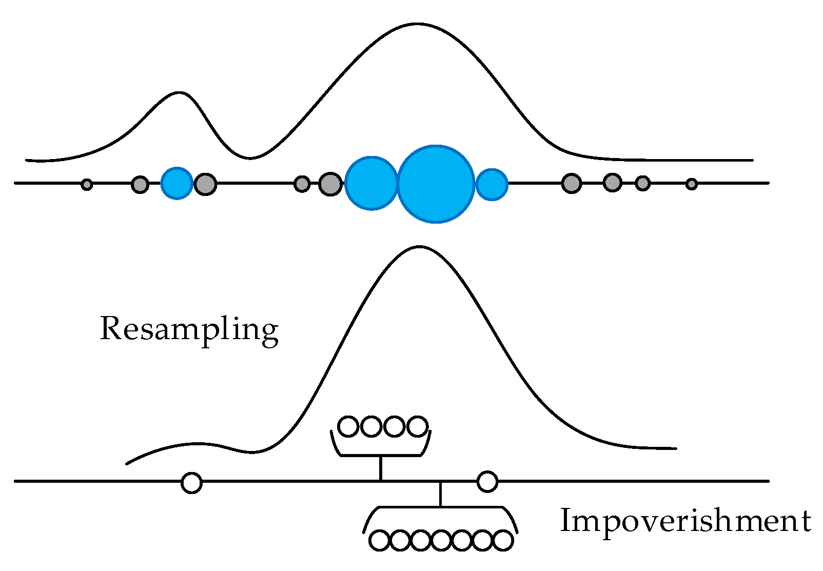
2.2. Particle Filter Method

The PF approach is an implementation of Bayesian filtering by Sequential Monte Carlo (SMC) sampling. The main idea is to express the required posterior pdf of state variables by a set of random particles with associated weights. As the number of particles increases, the true posterior pdf of state variables is equivalently approached [26]. In detail, consider a mass of particles { x t i , w t i } i = 1 N are sampled from the posterior pdf p ( x t | y 1 : t ) , where N is the particle number, x t i represents the random state variables, and w t i denotes the associated weight. The posterior pdf of the state variables is approximated as a discrete function:
p ( x t | y 1 : t ) i = 1 N w t i δ ( x t x t i ) ,
where δ ( · ) is the Dirac delta function.
For the most nonlinear systems, the analytic solution for the posterior pdf p ( x t | y 1 : t ) is often difficult to obtain. To deal with the difficulty in sampling indirectly from the posterior pdf, the sequential importance sampling (SIS) method, which is the basic PF form, is often adopted. The particles are generated from a known importance density, also called proposal distribution, which is easily sampled and represented by q ( x t | y 1 : t ) . The importance weight for each particle is updated in a recursive form, as follows:
w t i = w t 1 i p ( y t | x t i ) p ( x t i | x t 1 i ) q ( x t i | x t 1 i , y t ) ,
Equation (6) provides the mechanism to sequentially update the importance weights, given an appropriate choice of the proposal distribution q ( x t i | x t 1 i , y t ) . Consequently, the choice of the proposal distribution is one of the most critical issues in the design of PF. The optimal proposal density makes the variance of importance weights minimal and significantly improves the efficiency of PF. An appropriate choice for the proposal distribution is usually expressed for simplicity as follows:
q ( x t i | x t 1 i , y t )   =   p ( x t i | x t 1 i ) ,
When the transitional prior pdf is chosen as the proposal distribution, the importance weights only depend on their past values and the likelihood p ( y t | x t i ) . Then, the weights updating formula in Equation (6) is reduced to
w t i = w t 1 i p ( y t | x t i ) ,
The normalized weight is calculated by
w ˜ t i = w t i i = 1 N ( w t i ) 2 ,

2.3. Problem Formulation

The degeneracy phenomenon is one of the major drawbacks of the basic PF scheme. In fact, after a few iterations, all but one particle have negligible weights. These particles’ contribution to the approximation of the posterior pdf is close to zero. This implies that a large computational resource is wasted to update these particles. The degeneracy of PF is measured by the effective sample size N e f f [26], which is defined by
N e f f = 1 i = 1 N ( w ˜ t i ) 2 ,
where w ˜ t i is the normalized weight. According to the N e f f definition, the smaller N e f f indicates the more severe degeneracy. To solve the particle degeneracy problem, a resampling procedure is usually adopted in the PF. This process eliminates the particles with small important weights and replaces them by multiplying particles with large weights. The process is illustrated in Figure 1. In the past decades, various resampling methods have been proposed in literature, and the most commonly used are multinomial resampling, stratified resampling, and residual resampling [13]. After the resampling process, all particles are the same weight. Thus, the posterior pdf is approximated by
p ( x t | y 1 : t ) 1 N i = 1 N δ ( x t x t i ) ,
However, the other serious problem is particle impoverishment sparked by the resampling method. In Figure 1, the solid circles represent the parent particles and the hollow circles denote the offspring particles. The size of the circles represents the corresponding weights of the particles. The blue solid circles are selected particles and the grey solid circles are eliminated particles. The above curve is the prior pdf, and the curve shown below presents the true posterior pdf. As described in Figure 1, in the resampling procedure, only the particles with large weights are selected as the parent particles, others are abandoned. The offspring particles are replicas of the selected particles. This procedure may lead to a dramatic loss of diversity of the offspring particles, characterized by the new particles sharing a few distinct values gathering at a few select places. In other words, after several recursive calculations, the new particle set is difficult to reflect the true posterior pdf. Therefore, how to make appropriate changes to the multiplicative particles according to certain rules to obtain diversity and reduce impoverishment is the core issue. This is the original idea of the modified particle filter algorithm based on the biological immune system.

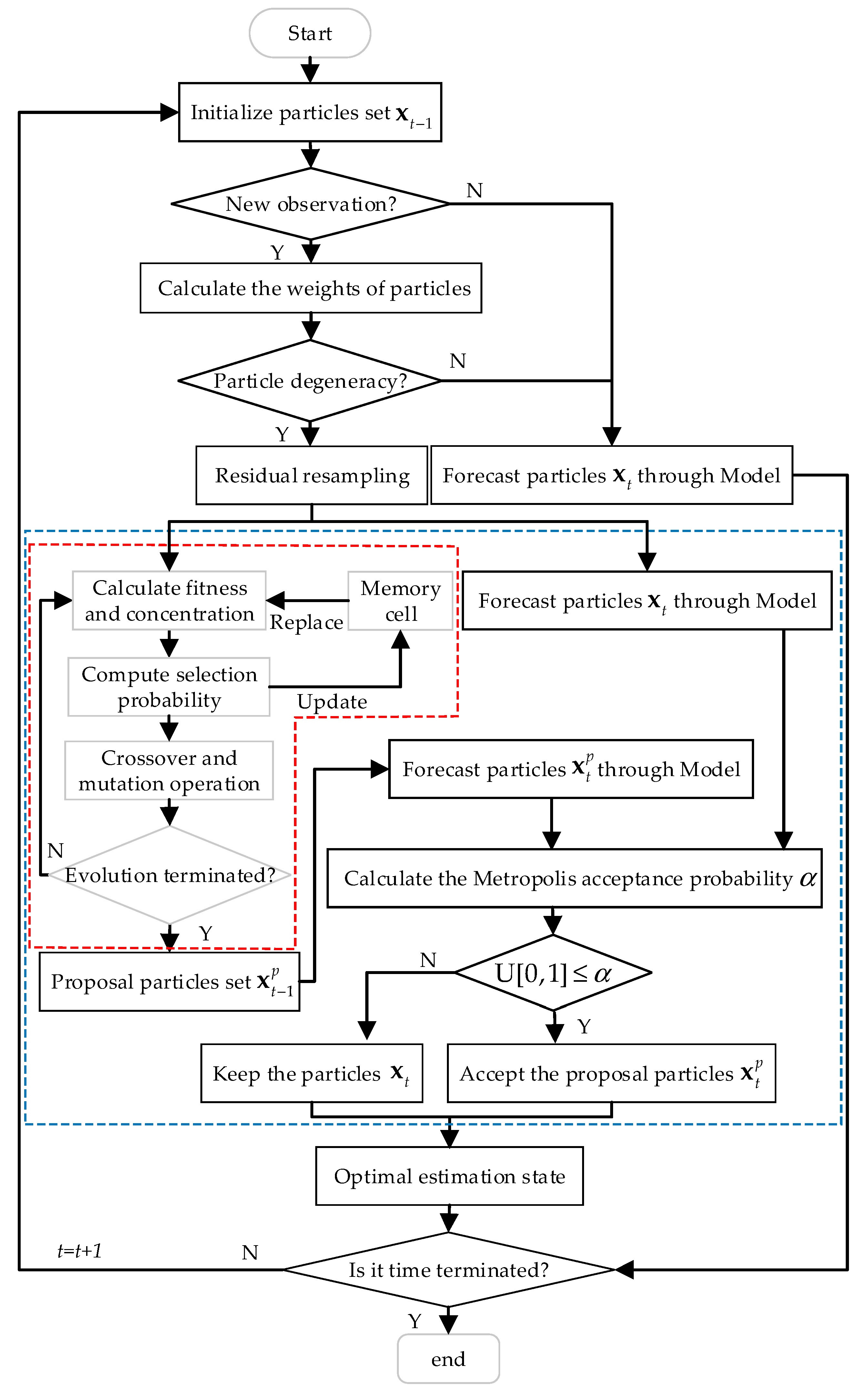
2.4. Immune Evolution Particle Filter with MCMC

2.4.1. Immune Evolution Algorithm (IEA)

The immune system is a multifunction biological defense system, which has evolved to protect bodies against infections from viruses, bacteria, fungi, and also worms and tumor cells [27]. Once pathogens invade the body, they will become antigens and provoke the immune response. When the immune system detects the foreign invasive antigens, the immune cells will propagate a mass of cloned antibodies. The cloned antibodies are selected from the top candidate antibodies listed in descending order by selection probability. Through the division and differentiation of cells, immune cells generate diverse antibodies to destroy the antigens. During the immune study process, the cells propagating the antibodies will be saved as memory cells. When the same or similar antigens appear again, the memory cells will quickly react and produce better antibodies [28]. The immune memory is the distinct feature of the immune system.
The artificial immune evolution algorithm is a type of algorithm inspired by biological immune system theories. It simulates the adaptive capacity of the immune system to propagate antibodies against the foreign invasive antigens. It implements the recognition of invasive antigens, and the generation of diverse antibodies, immune memory, self-regulation, and other functions [29]. There have been many successful applications of IEA, such as optimization, data mining, video target tracking, industrial applications, and Internet of Things services [29,30,31,32].

2.4.2. Immune Evolution Particle Filter Proposed

The aim of this study is solving the particle impoverishment problem. Based on the same demand of improving individual diversity and quality, PF and immune evolution can be linked together. Corresponding to the biological immune system, the foreign invasion antigens indicate the state or parameters of optimal problems to be solved; the antibodies generated by the immune system represent the candidate particles for the variable estimation. The distinct features, which are useful for improving diversity, are discussed below.
Similar to the basic GA, the immune system produces offspring antibodies by genetic operators such as selection, crossover, and mutation. However, the selection process is not only according to the fitness of individuals, but also considering the diversity of the selected ones. According to the crossover rate, parent antibodies exchange part of their information to generate the new offspring antibodies. The crossover operator expands the search space of candidate solutions and finally achieves the global search purpose. At the same time, the mutation may also happen in the offspring antibodies, according to the mutation rate. This process produces new genes which are not included in the initial population, or recovered genes lost during the selection. The mutation operator maintains population diversity and prevents premature convergence. This antibody diversity preservation mechanism is worth learning to solve the impoverishment problem of standard PF. Until reaching the termination condition, the iteration is finished.
In practice, as the first step of this mechanism implementation, the particle selection is implemented to achieve the goal of promotion and suppression of particles based on the fitness and the concentration. The term fitness measures the degree of matching between observations and candidate particles by fitness function. The term concentration indicates the similarity degree of the particle with other particles by concentration function. The particles with higher fitness will be promoted and the ones with higher concentration will be suppressed. In this way, the diversity of particles is further ensured. Thus, the problem of super individuals is mitigated and the solution space is extended. In addition, inspired by the immune system, the immune memory is designed to store the optimal particles and generate better offspring particles for each iteration.
The abovementioned diversity preservation idea, immune memory, and genetic operators are adopted in the proposed algorithm IEPFM. These functions need to be improved to fit the particle filter in DA. Figure 2 displays the algorithm process of IEPFM. The idea of immune evolution is described in the red dotted frame. Note that the aim of immune evolution process is creating new candidate particles for MCMC simulation, which happens after residual resampling.
The detailed assimilation process includes the following steps:
Step (1). At the assimilation initial time step t = 0 initializes particle set { x 0 i , w 0 i } i = 1 N from the state variable prior pdf p ( x 0 ) , where w 0 i = 1 / N .
Step (2). The particles set state propagates according to the model and particle set { x t 1 i , w t 1 i } i = 1 N . The new particles { x t i , w t i } i = 1 N are forecasted through model, where w t i = 1 / N .
Step (3). If the new observation is available at current time step t , use the new observation to calculate the selection probability of particles. Otherwise, skip to step (13) and the final estimated state is obtained.
Step (4). At each observation time, the memory cell is constructed. The length of memory cell is M , half of the total number of particles (i.e., M = N / 2 ).
Step (5). In this study, the fitness is proportional to the likelihood. However, a common choice of the likelihood density function is the Gaussian distribution that describes the misfit between the state predictions x t i and the observations y t , scaled by the (usually a priori defined) standard deviation of the observation error σ [17]. Thus, the fitness can be estimated as follows:
f i t n e s s t i = ( 1 2 π σ ) m exp ( ( y t x t i ) T ( y t x t i ) 2 σ 2 ) ,
Step (6). Calculate the normalized weights of particles { x t i , w ˜ t i } i = 1 N according to (8) and (9). Then, the effective sample size N e f f can be calculated according to (10). If N e f f N r , go to the next step, otherwise, forecast particles { x t i , w t i } i = 1 N through the model and skip to step (13).
Step (7). Calculate the concentration of particles as follow:
C t i = n simi N ,
where n simi is the number of particles with high affinity of particle i . Particles with high concentration should reduce their chosen probability, and vice versa.
Step (8). The selection probability of each particle is obtained as:
p choose = ω p fit + ( 1 ω ) p con = ω f i t n e s s t i j = 1 N f i t n e s s t j + ( 1 ω ) C i β ,
where ω and β are adjustment constants. In IEPFM, the selection probability of each particle is determined by its fitness and concentration. Then, the particle set will be sorted by selection probability. The optimal particle, which has the highest selection probability, will be stored in the memory cell at every iteration. If the memory cell is full, the worst particle of them will be replaced.
Step (9). Crossover can operate between two cross parents, which are selected randomly according to the crossover probability p c . Considering the state of double-coding and the simplicity, parent particles produce offspring by linear arithmetic crossover. The crossover operator is defined as:
{ x 1 = k x 1 + ( 1 k ) x 2 x 2 = ( 1 k ) x 1 + k x 2 ,
where k is a random number generated from the interval [ 0 , 1 ] .
Step (10). Mutation strategy is simulated to promote the diversity of particles. Mutation can operate between two mutation parents, which are selected randomly according to the mutation probability p m . The mutation operator is expressed as:
x = 2 x H x L + ε ,
where x H and x L represent the particles with high and low selection probability, respectively; ε is a perturbation vector, which is drawn from the uniform distribution on U ( b , b ) with b , which is small compared to the width of the target distribution.
Step (11). Cycle from step (5) to step (10) until the maximum evolution generation is achieved. Otherwise, use MCMC simulation to obtain optimal particle set { x ^ t i , w ^ t i } i = 1 N , where { w ^ t i } i = 1 N = 1 / N . Further details are described below.
Step (12). Calculate the optimal estimate state as
x ˜ t = i = 1 N x ^ t i × w ^ t i ,
Step (13). If time step is terminated, the whole process stops. Otherwise, make t = t + 1 and return to step (2), and cycle the above procedures.

2.4.3. Markov chain Monte Carlo (MCMC) Simulation

The MCMC and sequential Monte Carlo methods have emerged as the two main tools to sample high dimensional probability distributions [33]. The key idea of MCMC simulation is based on using Markov chain to explore the target distribution. The immune evaluation particle filter procedure generates candidate particles x t 1 p . Then, each candidate particle is re-evaluated from time t 1 to t by Equation (1), and the Metropolis acceptance probability α is used to determine whether to move from x t 1 to x t 1 p or not; α is calculated as follows
α = min ( 1 , p ( y t | x t p ) p ( y t | x t ) ) ,
Only when μ α , where μ U [ 0 , 1 ] , the candidate particle is accepted and replaces the old particle. After the IEPFM process, the new particle set will have a distribution closer to the posterior pdf, and will also have more diversity, thus reducing the potential of particle impoverishment.

3. Results and Discussion

In this section, firstly, the Lorenz96 model is used as the numerical simulation experiment to compare the performance of IEPFM with EnKF and DEPFM. Then, IEPFM is applied for soil moisture data assimilation. The performance of each method is evaluated against the true values using the average root mean square error (RMSE) over all state variables.

3.1. Lorenz96 Model Experiment

The Loren96 model [34] is a high dimensional and strongly nonlinear model often used to validate the new DA algorithms. This model simulates the time evolution of an atmospheric quantity and is described by the ordinary differential equations:
d x j d t = ( x j + 1 x j 2 ) x j 1 x j + F , j = 1 , 2 , J ,
The cyclic boundary conditions are defined by x 1 = x J 1 , x 0 = x J and x 1 = x J + 1 ; F is a constant external forcing term, which is usually chosen as F = 8 for high chaotic behavior.
In this paper, the 40 dimensions Lorenz96 model is chosen for the experiment. The fourth-order Runge-Kutta scheme with a step of Δ t = 0.05 , corresponding to six hours in real life, is used to integrate the model. The model is initialized by choosing F = 8 , except for F = 8.01 at variable x 20 , and running for 1000 time steps. The end states of that run are considered as the initial condition for the DA experiment. The true state variables are obtained by integrating the model. All of the model state variables are observed every five time steps and added to the Gaussian observational noise with error covariance σ obs 2 = 0.2 . The initial particles or ensembles are generated by adding the Gaussian noise with initial covariance σ init 2 = 0.1 . The model error covariance is σ model 2 = 0.1 .

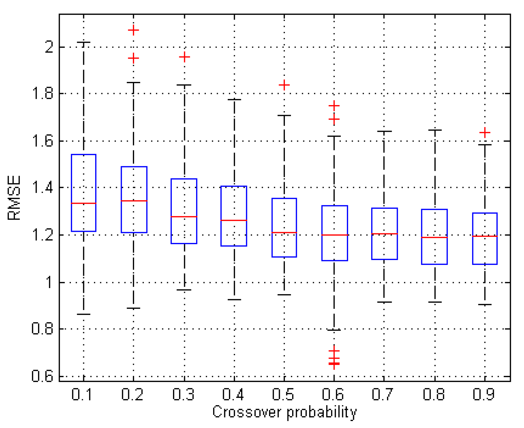
3.1.1. Sensitivity Analysis

To further understand the influence of key parameter settings of IEPFM, a set of experiments are conducted for sensitivity analysis. The average RMSEs are used to evaluate the performance of each setting average for 30 independent runs. The crossover probability p c is varied from 0.1 to 0.9 by steps of 0.1. The experimental results are summarized in Figure 3. For the same mutation probability, the value of RMSE is near 1.2 when p c 0.5 . The lowest RMSE is obtained when p c =   0.8 . Thus, p c =   0.8 is selected for IEPFM.
The same as the crossover probability, the mutation probability ranges from 0.1 to 0.9 steps by 0.1, and the corresponding RMSEs are presented by box plots in Figure 4. It is clearly observed that the results are almost unanimously obtained when p m 0.3 . Therefore, the parameter setting of crossover and mutation probability has no significant impact on IEPFM as a result of MCMC simulation. This conclusion is consistent with that drawn by Abbaszadeh et al. [23]. In this study, p c = 0.8 and p m = 0.3 are adopted, since RMSE resulting from this setting is slightly better.
As for the size of the particle set, Figure 5 gives bar plots of the RMSEs and computing time for different ensemble sizes (i.e., 25, 50, 100, 150, and 200) for 30 independent runs. As shown in Figure 5, the RMSE gradually decreases and computing time sharply increases, along with ensemble size becoming larger. It can be found that the performance of IEPFM improves as the ensemble size increases. But the RMSE shows almost no obvious change since N > 100. After comprehensive consideration of RMSE and computing time, ensemble size is set to 100 in this study.

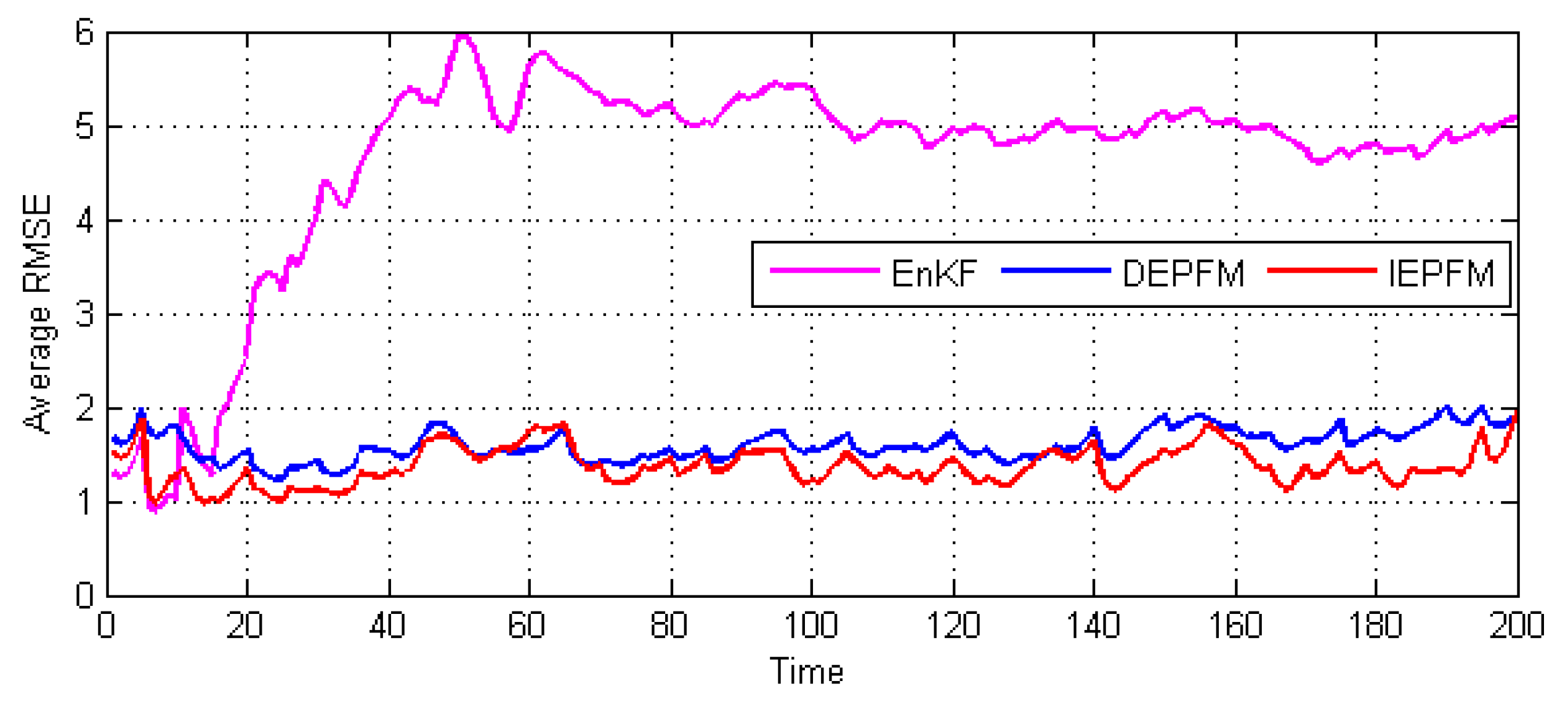
3.1.2. Performance Comparisons

Three DA algorithms with different particles or ensemble members are simulated for 200 time steps and the state variables are estimated by assimilating the observations into the Lorenz96 model. All 40 state variables are selected for comparison. The average RMSEs of 30 independent runs are used to evaluate the performance of DA algorithms. In addition, for IEPFM, the crossover probability p c and the mutation probability p m are set to 0.8 and 0.3, respectively. The parameters of DEPFM are referred to Vrugt et al. [25]. Table 1 shows the experiment results of EnKF, DEPFM, and IEPFM with different ensemble size. From Table 1, it can be observed that EnKF performs poorly in the highly nonlinear dynamics model. However, the particle filters with MCMC simulation improve filter performance significantly, and the REMSs diminish with the increment of the ensemble size. The best state estimation results belong to IEPFM, which offers the lowest RMSE at all different ensemble sizes, as shown in the table.
To intuitively present the effectiveness of IEPFM, the average RMSE (N = 100) of every time step is displayed in Figure 6. As shown in Figure 6, the state values are not correctly estimated by EnKF, except for the beginning of the assimilation. This is most likely because normal distribution is assumed to derive from EnKF analysis scheme, limiting its performance for nonlinear and non-Gaussian models. IEPFM gives much more accurate estimation results than EnKF and DEPFM.

3.1.3. Comparison of Computation Time

To compare the complexity of the three different algorithms, the average computation time corresponding to Table 1 is provided in Figure 7. It is clearly seen that the computation time increases with the increments of ensemble size. The obvious difference is that EnKF increases asymptotically and approximately linearly. However, the computation time of other methods increases rapidly when the ensemble size is greater than 100. This finding is of no surprise, since the IEPFM and DEPFM are combining PF with MCMC simulation, which improve particles diversity through differential evolution or immune evolution during the filtering process. From Figure 7, EnKF is the most efficient, computationally, and IEPFM the least. It is not hard to see from Table 1 that EnKF exhibits rather poor precision. In addition, the gap between IEPFM and DEPFM grows from ensemble size N = 150, since IEPFM searches solution space based on crossover and mutation, and spends time on sorting particles. Considering the RMSE index and computation time, IEPFM is suitable for assimilation of high dimensional and nonlinearity problems for much smaller ensemble size.

3.2. Soil Moisture Data Assimilation Experiment

3.2.1. Study Area

To understand land-atmosphere interactions of the Tibetan Plateau and their influence on the climate of South-East Asia, the SM monitoring of this region is most important. The Tibetan Plateau observatory of plateau scale soil moisture and temperature consists of three regional scale in situ reference networks, including the Maqu network, the Naqu network, and the Ngari network. The Maqu network was installed on the north-eastern fringe of the Tibetan Plateau (33°30′–34°15′N, 101°38′–102°45′E) in July 2008. The network is located in the Yellow River Source Region and in the south of Maqu County in the Gansu province, China (Figure 8). It is also helpful for water management sustainability research, such as reducing river sedimentation, soil water retention, and flood mitigation of the Yellow River [35]. It covers the large valley of the Yellow River and the hills around it, which are characterized by a uniform land cover of short grassland grazed by sheep and yaks. In this area, the elevations of stations range from 3430 m to 3750 m above mean sea level. According to the Koeppen Classification System, this site has a cold and wet climate, with rainy summers and dry winters due to monsoons [36].

3.2.2. The Land Surface Model and Data Preparation

The LSM used in this study is the Variable Infiltration Capacity (VIC) model. The VIC model is a semi-distributed LSM accounting for the balances of water and energy, originally developed jointly at the University of Washington and Princeton University. It is a grid cell based macroscale hydrology model used to simulate various hydrologic variables, such as SM, evapotranspiration, snow accumulation and melt, runoff, baseflow, and various heat fluxes [37]. The surface runoff and baseflow are subsequently routed through the river network based on grids, and simulate streamflow at selected points within the basin. The model can run either at a sub-daily time step with a full energy balance, or at daily time step in water balance mode.
This study performs the VIC model version 4.2.c. In order to drive the model, VIC requires meteorological forcing files, vegetation data, and soil information for each grid cell. The meteorological forcing files, including at least precipitation, maximum and minimum temperature, and the average wind speed, are extracted from the China ground climate daily dataset (version 3.0) developed by the China Meteorological Information Center. The vegetation information is obtained from Maryland land cover dataset and the soil information is gathered from the China Soil Map Based Harmonized World Soil Database (version 1.1) provided by Cold and Arid Regions Sciences Data Center at Lanzhou (http://westdc.westgis.ac.cn).
To obtain the VIC model parameters of the study area, simulations were performed over the Source Region of the upper Yellow River in China at a spatial resolution of 0.25°, which made 250 model grid cells. The VIC model was calibrated by forcing the model and adjusting parameters that govern infiltration and baseflow recession to match simulated streamflow, with naturalized observations obtained from the selected hydrologic station in the same recording period of 2007–2013. The assumption made is that the adjusted parameters are the optimal values, and keep constant in the following experiment.

3.2.3. Observations Preparation

The Maqu network spans an area of approximately 40 km × 80 km, covering more than one resolution grid cell. In the study area, the observed soil moisture of participating assimilation grid cells is calculated from monitoring sites by inverse distance weighted interpolation method. Since the depth of top soil layer of VIC model is 10 cm and all record data of the Maqu network is at least at 5 and 10 cm, the only soil moisture at 10 cm is updated by the assimilation of observed soil moisture. When assimilating the weighted mean of in situ SM data, the biases between the single point measurement-based and model-based SM cannot be avoided. The bias correction is necessary and required before assimilation experiment. In this paper, the cumulative distribution function (CDF) matching technique is used to rescale the in situ soil moisture into the VIC model space. Finally, the VIC model begins to run from March 1, 2011, to eliminate the spin-up period, but only the data after March 31, 2012, is it used for the data assimilation experiments at daily time step.

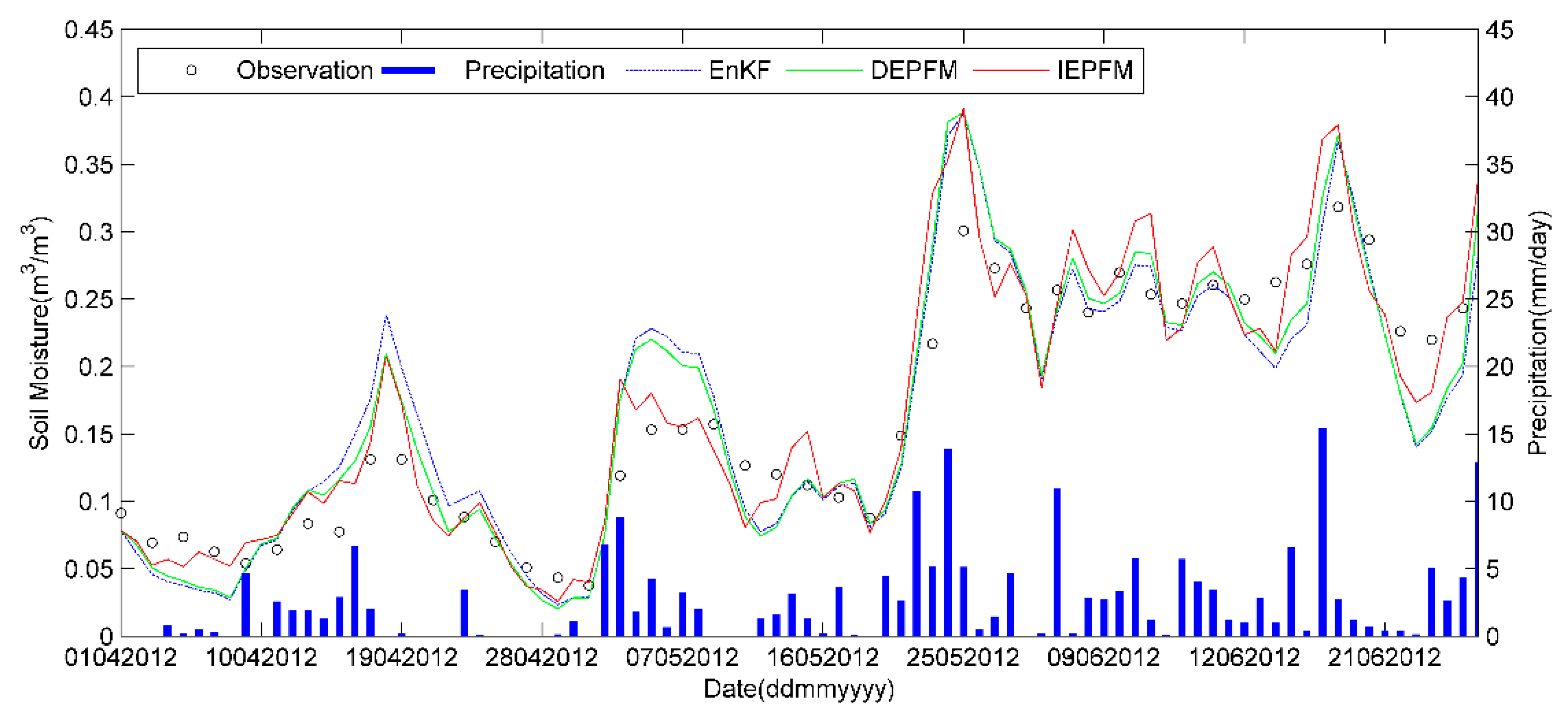
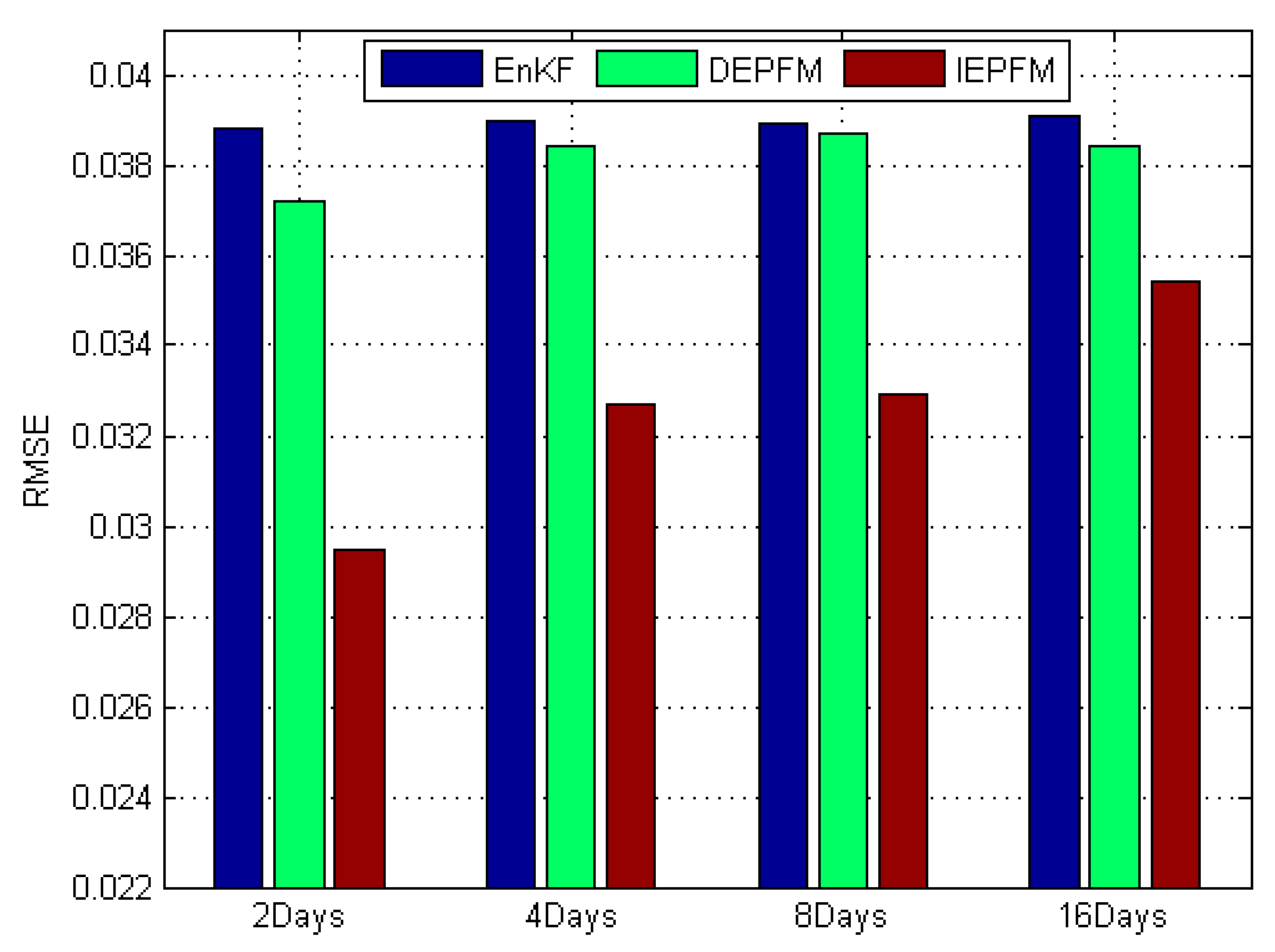
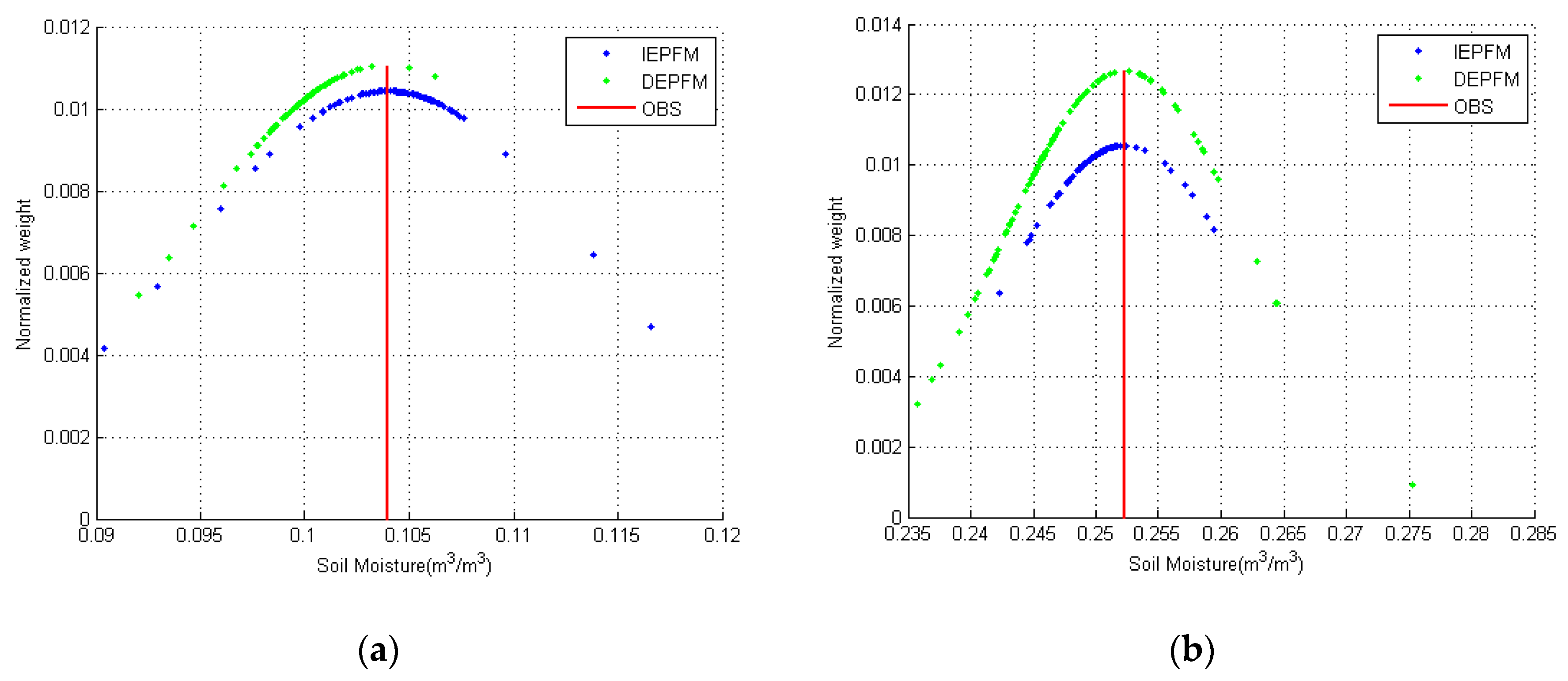
3.2.4. Results and Analysis

The SM assimilation experiments are performed to assess whether IEPFM can improve the VIC model simulations better than other DA methods in the forecast period. The focus is on the effectiveness of IEPFM in solving particle impoverishment. The classical assimilation algorithms EnKF and DEPFM are used to assimilate observed data into the VIC model to estimate surface SM on a daily time step scale. Then, the forecast results of three DA methods are compared with the observations. The ensemble size is set to 100 and the initial particles are sampled from a Gaussian distribution with mean zero and standard deviation σ mod el = 0.05 , obtained from the model error. According to the specific calibration result of the Maqu network, the RMSE is reduced from 0.06 to 0.02 m3/m3, which can be considered as the absolute accuracy of each station of this network [36]. One option is to use this accuracy value to characterize the observation error, which is same across the three methods. The other parameters of evolution algorithms are followed to the numerical simulation experiment.
1. Soil moisture analysis
The DA improvements of EnKF, DEPFM, and IEPFM are assessed by comparing the simulations to the in situ soil moisture observations every two days, shown in Figure 9. The daily precipitation data is also displayed during the simulation period, represented by stem plots in the figure. Figure 9 indicates the following points: Firstly, the results of the three assimilation methods can reflect the overall change trend of the surface SM. It is not hard to see that strong consistency exists between the change trend of SM and the precipitation data. Especially with the increase of precipitation, the SM obviously increases in the flood season in June. In that period, the gap between the model simulation result with DA and observations has increased. According to the forecast SM curves of the three methods, it could be clearly seen that IEPFM generates the most accurate SM, followed by DEPFM, and EnKF produces the worst results farthest from the observations.
2. Performance metrics
The evaluation of the three DA methods’ performance is based on the three metrics: the RMSE, the mean absolute bias (MAB), and the correlation coefficient (R). The lower RMSE or MAB, and the greater R, indicate better performance of forecast SM. Table 2 presents the RMSE (m3/m3), the MAB (m3/m3), and the R (−) of the three DA methods. The conclusion can be drawn that IEPFM algorithm leads to the best statistic scores for the assimilation experiment. IEPFM shows a strong correspondence with the observation, as indicated by the highest correlation (0.9502) and the lowest RMSE (0.0295 m3/m3) and MBA (0.0225 m3/m3). As revealed by Table 2, the forecast SM obtained from IEPFM is closer to the observed data than DEPFM and EnKF.
3. Assimilation frequency analysis
In order to further understand the effects of different assimilation frequencies on prediction, four experiments were designed. When other assimilation parameters were consistent, only the assimilation cycles of four group experiments changed following every two days, four days, eight days, and sixteen days. It meant that only one observation was available and could be assimilated into model per cycle. The results of experiments are illustrated in Figure 10. Overall, similar trends can be observed. With the extension of assimilation cycle, the prediction error increases. As shown in the figure, IEPFM performs best with the lowest RMSE among the three algorithms, no matter how the assimilation cycle changes, and DEPFM produces more accurate predictions than EnKF.
4. Particles diversity analysis
The particle diversity based on IEPFM is illustrated in Figure 11. Two subfigures describe the particles and their associated normalized weights of assimilation experiment using DEPFM and IEPFM when the assimilation time steps are t = 45 and t = 70. Although it is difficult to directly judge the accuracy of the two algorithms from the figure, it is clear that particles generated by the two methods are able to represent the true posterior distributions. In each figure, the green and blue particles concentrate the surrounding regions of observation, which also indicates the convergence to the estimates. Overall, the blue particle’s aggregation curve of IEPFM is below, and covered with the green curve of DEPFM in Figure 11. This means that blue particles tend to gather to a more limiting and actual target distribution, and IEPFM generates more diversity particles with large weights. In addition, the MCMC move step is used to reject the particles which move outside the true posterior distributions and accept the particles with excellent performance. Through the process of IEPFM, most of the particles with normalized weights less than 0.04 are eliminated, and the large-weight particles are preserved and evolved.
The scatter diagram Figure 12 is selected for illustration of the particle’s diversity performance in another way. From the figure, it is hard to find the phenomenon of particle impoverishment characterized by many particles sharing the same values, clustering together at a few places, like erect short line segments. Because of crossover and mutation, particles could maintain the diversity and avoid collapsing local optimums. Figure 12 also exhibits that blue particles scatter around the observations and their location center is closer to the observation than green particles. In summary, after genetic operation and MCMC moves in IEPFM procedure, the diversity of particles are promoted.

4. Conclusions

An IEPFM algorithm inspired by the biological immune system has been proposed in this paper to alleviate the particle impoverishment problem of the general PF. The distinguishing feature of IEPFM is a special strategy of generating candidate particles for MCMC move step based on the immune evolution concept. The performance of the proposed IEPFM in estimating the posterior state variables is validated through the two case studies, including the high dimensional and strongly nonlinear atmospheric model and the VIC hydrological model. This study obtains the following findings.
Both assimilation results demonstrate that IEPFM consistently receives the best performance compared with EnKF and DEPFM. The candidates with more prior information may lead to more accurate posterior distribution of state variables during particle evolution procession. The ability of MCMC simulation also improves adequate particle diversity, thus the particle impoverishment problem is mitigated.
An important and interesting finding is that the performance of IEPFM appears almost unaffected by the setting of crossover probability and mutation probability, which are the key parameters of the immune evolution algorithm. Based on this finding, crossover and mutation suggested probabilities are set to 0.8 and 0.3, respectively. The benefit of this approach is in reducing the influence of subjective setting of key parameters on algorithm performance.
Additionally, the ensemble size of particles set to 100 receives similar RMSE as the larger size. This finding is useful for decreasing computational time of IEPFM, since the computational demand increases rapidly when particle number exceeds this value.
Finally, it is not difficult to see that EnKF behaves differently in the two experiments. The performance is not improved significantly with the increase of ensemble size. The results indicate that EnKF has limitations in dealing with strongly nonlinear systems.
However, IEPFM will be validated further with other observations, such as brightness temperatures. Furthermore, some improvements could be made on IEPFM and VIC model. The parameters of VIC model also impact the efficiency of assimilation. Thus, the optimization problem of these model parameters will probably be investigated in the future.

Author Contributions

Conceptualization & methodology, F.J. and R.A.; validation, F.J. and Y.S.; investigation, F.J. and Y.S.; software, F.J; writing—original draft preparation, F.J.; writing—review and editing, R.A. and Y.S.; funding acquisition, R.A.

Funding

This research is funded jointly by the Key Project in the National Science & Technology Pillar Program during the Twelfth Five-Year Plan Period, grant number 2013BAC03B04; the National Natural Science Foundation of China, grant number 41871326 and 41271361.

Acknowledgments

The authors would like to thank Prof. Su and Dr. Zeng for kindly providing the in situ data. The authors also thank the anonymous reviews for their critical reviews and constructive comments.

Conflicts of Interest

The authors declare no conflict of interest.

References

  1. Parrens, M.; Wigneron, J.P.; Richaume, P.; Mialon, A.; Al Bitar, A.; Fernandez-Moran, R.; Kerr, Y.H. Global-scale surface roughness effects at L-band as estimated from SMOS observations. Remote Sens. Environ. 2016, 181, 122–136. [Google Scholar] [CrossRef]
  2. Brocca, L.; Ciabatta, L.; Massari, C.; Camici, S.; Tarpanelli, A. Soil Moisture for Hydrological Applications: Open Questions and New Opportunities. Water 2017, 9, 140. [Google Scholar] [CrossRef]
  3. Kirby, J.M.; Mainuddin, M.; Ahmad, M.D.; Gao, L. Simplified Monthly Hydrology and Irrigation Water Use Model to Explore Sustainable Water Management Options in the Murray-Darling Basin. Water Resour. Manag. 2013, 27, 4083–4097. [Google Scholar] [CrossRef]
  4. Lievens, H. SMOS soil moisture assimilation for improved hydrologic simulation in the Murray Darling Basin, Australia. Remote Sens. Environ. 2015, 168, 146–162. [Google Scholar] [CrossRef] [Green Version]
  5. Huang, C.; Xin, L.; Ling, L. Retrieving soil temperature profile by assimilating MODIS LST products with ensemble Kalman filter. Remote Sens. Environ. 2008, 112, 1320–1336. [Google Scholar] [CrossRef]
  6. Moradkhani, H. Hydrologic remote sensing and land surface data assimilation. Sensors 2008, 8, 2986–3004. [Google Scholar] [CrossRef] [PubMed]
  7. Dumedah, G.; Coulibaly, P. Evolutionary assimilation of streamflow in distributed hydrologic modeling using in-situ soil moisture data. Adv. Water Resour. 2013, 53, 231–241. [Google Scholar] [CrossRef]
  8. Weerts, A.H.; El Serafy, G.Y.H. Particle Filtering and Ensemble Kalman Filtering for state updating with hydrological conceptual rainfall runoff models. Water Resour. Res. 2006, 42, 123–154. [Google Scholar] [CrossRef]
  9. Evensen, G. Sequential data assimilation with a nonlinear quasi-geostrophic model using Monte Carlo methods to forecast error statistics. J. Geophys. Res. Ocean. 1994, 99, 10143–10162. [Google Scholar] [CrossRef]
  10. Gordon, N.J.; Salmond, D.J.; Smith, A.F.M. Novel approach to nonlinear/non-Gaussian Bayesian state estimation. IEE Proc. F Radar Signal Process. 1993, 140, 107–113. [Google Scholar] [CrossRef]
  11. Montzka, C.; Moradkhani, H.; Weihermüller, L.; Franssen, H.J.H.; Canty, M.; Vereecken, H. Hydraulic parameter estimation by remotely-sensed top soil moisture observations with the particle filter. J. Hydrol. 2011, 399, 410–421. [Google Scholar] [CrossRef]
  12. Mattern, J.P.; Dowd, M.; Fennel, K. Particle filter-based data assimilation for a three-dimensional biological ocean model and satellite observations. J. Geophys Res. Ocean. 2013, 118, 2746–2760. [Google Scholar] [CrossRef] [Green Version]
  13. Fan, Y.R.; Huang, G.H.; Baetz, B.W.; Li, Y.P.; Huang, K.; Li, Z.; Xiong, L.H. Parameter uncertainty and temporal dynamics of sensitivity for hydrologic models: A hybrid sequential data assimilation and probabilistic collocation method. Environ. Model. Softw. 2016, 86, 30–49. [Google Scholar] [CrossRef]
  14. Hartanto, I.M.; Van Der Kwast, J.; Alexandridis, T.K.; Almeida, W.; Song, Y.; van Andel, S.J.; Solomatine, D.P. Data assimilation of satellite-based actual evapotranspiration in a distributed hydrological model of a controlled water system. Int. J. Appl. Earth Obs. Geoinf. 2017, 57, 123–135. [Google Scholar] [CrossRef]
  15. Vrugt, J.A.; ter Braak, C.J.; Diks, C.G.; Schoups, G. Hydrologic data assimilation using particle Markov chain Monte Carlo simulation: Theory, concepts and applications. Adv. Water Resour. 2013, 51, 457–478. [Google Scholar] [CrossRef]
  16. Elsheikh, A.H.; Hoteit, I.; Wheeler, M.F. A nested sampling particle filter for nonlinear data assimilation. Q. J. R. Meteorol. Soc. 2014, 140, 1640–1653. [Google Scholar] [CrossRef]
  17. Plaza Guingla, D.A.; Pauwels, V.R.; De Lannoy, G.J.; Matgen, P.; Giustarini, L.; De Keyser, R. Improving particle filters in rainfall-runoff models: Application of the resample-move step and the ensemble Gaussian particle filter. Water Resour. Res. 2013, 49, 4005–4021. [Google Scholar] [CrossRef] [Green Version]
  18. Bi, H.; Ma, J.; Wang, F. An Improved Particle Filter Algorithm Based on Ensemble Kalman Filter and Markov Chain Monte Carlo Method. IEEE Trans. Geosci. Remote Sens. 2015, 53, 6134–6147. [Google Scholar] [CrossRef]
  19. Dumedah, G.; Coulibaly, P. Integration of an evolutionary algorithm into the ensemble Kalman filter and the particle filter for hydrologic data assimilation. J. Hydroinf. 2014, 16, 74–94. [Google Scholar] [CrossRef]
  20. Mechri, R.; Ottlé, C.; Pannekoucke, O.; Kallel, A. Genetic particle filter application to land surface temperature downscaling. J. Geophys. Res. Atmos. 2014, 119, 2131–2146. [Google Scholar] [CrossRef] [Green Version]
  21. Yin, S.; Zhu, X. Intelligent Particle Filter and Its Application to Fault Detection of Nonlinear System. IEEE Trans. Ind. Electron. 2015, 62, 3852–3861. [Google Scholar] [CrossRef]
  22. Qu, Y.; Qian, X.; Song, H.; Xing, Y.; Li, Z.; Tan, J. Soil Moisture Investigation Utilizing Machine Learning Approach Based Experimental Data and Landsat5-TM Images: A Case Study in the Mega City Beijing. Water 2018, 10, 423. [Google Scholar] [CrossRef]
  23. Abbaszadeh, P.; Moradkhani, H.; Yan, H.X. Enhancing hydrologic data assimilation by evolutionary Particle Filter and Markov Chain Monte Carlo. Adv. Water Resour. 2018, 111, 192–204. [Google Scholar] [CrossRef]
  24. Zhang, H.J. State and parameter estimation of two land surface models using the ensemble Kalman filter and the particle filter. Hydrol. Earth Syst. Sci. 2017, 21, 4927–4958. [Google Scholar] [CrossRef] [Green Version]
  25. Vrugt, J.A. Markov chain Monte Carlo simulation using the DREAM software package: Theory, concepts, and MATLAB implementation. Environ. Model. Softw. 2016, 75, 273–316. [Google Scholar] [CrossRef] [Green Version]
  26. Arulampalam, M.S.; Maskell, S.; Gordon, N.; Clapp, T. A tutorial on particle filters for online nonlinear/non-Gaussian Bayesian tracking. IEEE Trans. Signal Process. 2002, 50, 174–188. [Google Scholar] [CrossRef] [Green Version]
  27. Dudek, G. An Artificial Immune System for Classification with Local Feature Selection. IEEE Trans. Evolut. Comput. 2012, 16, 847–860. [Google Scholar] [CrossRef]
  28. De Castro, L.N.; Timmis, J.I. Artificial immune systems as a novel soft computing paradigm. Soft Comput. 2003, 7, 526–544. [Google Scholar] [CrossRef]
  29. Dasgupta, D.; Yu, S.H.; Nino, F. Recent Advances in Artificial Immune Systems: Models and Applications. Appl. Soft Comput. 2011, 11, 1574–1587. [Google Scholar] [CrossRef] [Green Version]
  30. Han, H.; Ding, Y.S.; Hao, K.R.; Liang, X. An evolutionary particle filter with the immune genetic algorithm for intelligent video target tracking. Comput. Math. Appl. 2011, 62, 2685–2695. [Google Scholar] [CrossRef] [Green Version]
  31. Wang, M.; Feng, S.; He, C.; Li, Z.; Xue, Y. An Artificial Immune System Algorithm with Social Learning and Its Application in Industrial PID Controller Design. Math. Probl. Eng. 2017. [Google Scholar] [CrossRef]
  32. Yang, Z.; Ding, Y.; Jin, Y.; Hao, K. Immune-Endocrine System Inspired Hierarchical Coevolutionary Multiobjective Optimization Algorithm for IoT Service. IEEE Trans. Cybern. 2018. [Google Scholar] [CrossRef] [PubMed]
  33. Andrieu, C.; Doucet, A.; Holenstein, R. Particle Markov chain Monte Carlo methods. J. R. Stat. Soc. 2010, 72, 269–342. [Google Scholar] [CrossRef] [Green Version]
  34. Lorenz, E.N. Predictability: A problem partly solved. Proc. Semin. Predict. 1995, 1, 1–18. [Google Scholar]
  35. Bryan, B.A.; Gao, L.; Ye, Y.; Sun, X.; Connor, J.D.; Crossman, N.D.; Liu, Z. China’s response to a national land-system sustainability emergency. Nature 2018, 559, 193–204. [Google Scholar] [CrossRef] [PubMed]
  36. Su, Z.; Wen, J.; Dente, L.; Velde, R.; Wang, L.; Ma, Y.; Hu, Z. The Tibetan Plateau observatory of plateau scale soil moisture and soil temperature (Tibet-Obs) for quantifying uncertainties in coarse resolution satellite and model products. Hydrol. Earth Syst. Sci. 2011, 15, 2303–2316. [Google Scholar] [CrossRef] [Green Version]
  37. Liang, X.; Lettenmaier, D.P.; Wood, E.F.; Burges, S.J. A simple hydrologically based model of land surface water and energy fluxes for general circulation models. J. Geophys. Res. Atmos. 1994, 99, 14415–14428. [Google Scholar] [CrossRef]
Figure 1. The particle impoverishment phenomenon caused by resampling procedure.
Water 11 00211 g001
Figure 2. The overview of IEPFM.
Water 11 00211 g002
Figure 3. Box plots of the RMSE with different crossover probability.
Water 11 00211 g003
Figure 4. Box plots of the RMSE with different mutation probability.
Water 11 00211 g004
Figure 5. Bar plots of the RMSE and computing time with the same conditions.
Water 11 00211 g005
Figure 6. Comparison of the assimilation results of average RMSE at every time step.
Water 11 00211 g006
Figure 7. Comparison of the average computation time at different ensemble sizes.
Water 11 00211 g007
Figure 8. (a) Location of the study area (black rectangle); (b) SRTM DEM of Maqu monitoring network and location of the monitoring sites of the network.
Water 11 00211 g008
Figure 9. Comparison of the assimilation results of EnKF, DEPFM, and IEPFM with VIC model.
Water 11 00211 g009
Figure 10. Bar plots of the RMSEs obtained by three methods with the same parameters and different assimilation frequencies.
Water 11 00211 g010
Figure 11. Comparison of the particle distribution and normalized weights produced by DEPFM and IEPFM on different assimilation days. (a) t = 45, (b) t = 70. The blue and green points present the particles generated by IEPFM and DEPFM, respectively. The corresponding SM of red line denotes the observation.
Water 11 00211 g011
Figure 12. Scatter diagrams of the particles generated by IEPFM and DEPFM on different assimilation days. (a) t = 45, (b) t = 70. The blue and green circles present the particles generated by IEPFM and DEPFM, respectively. The corresponding SM of red line denotes the observation.
Water 11 00211 g012
Table 1. Comparison of REMS for the Lorenz96 model.
Ensemble SizeEnKFDEPFMIEPFM
N = 25 4.62443.22362.4721
N = 50 4.62221.84391.8256
N = 100 4.61281.52601.3661
N = 150 4.67101.22421.1160
N = 200 4.66851.18641.1038
Table 2. Comparison of the performance of three DA algorithms.
DA AlgorithmsRMSEMABR
EnKF0.03880.03030.9103
DEPFM0.03720.02910.9181
IEPFM0.02950.02250.9502

