Systemic Flood Risk Management: The Challenge of Accounting for Hydraulic Interactions


__Kwakkel.png)
Abstract
1. Introduction
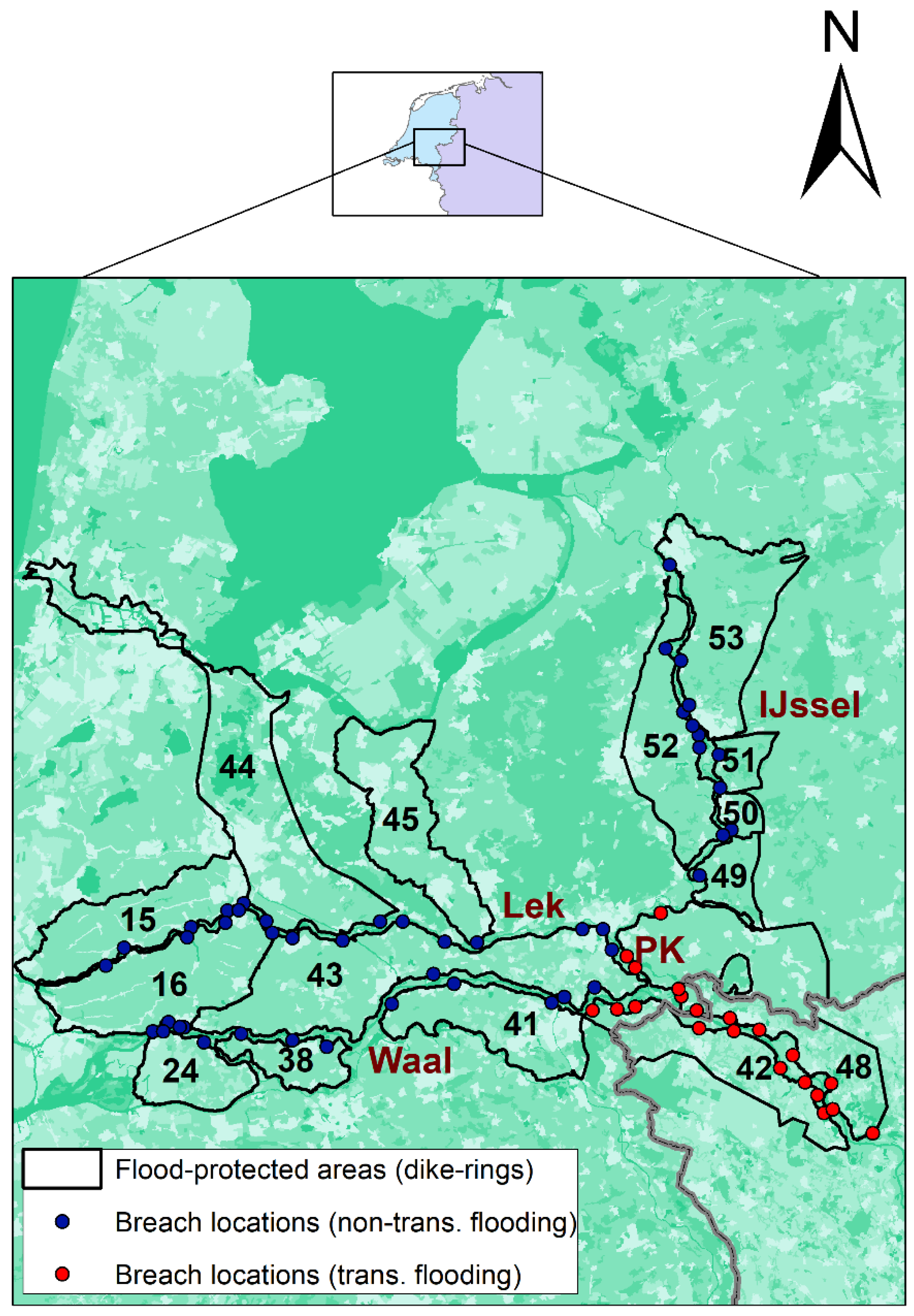
2. Case Study
3. Simulation Model
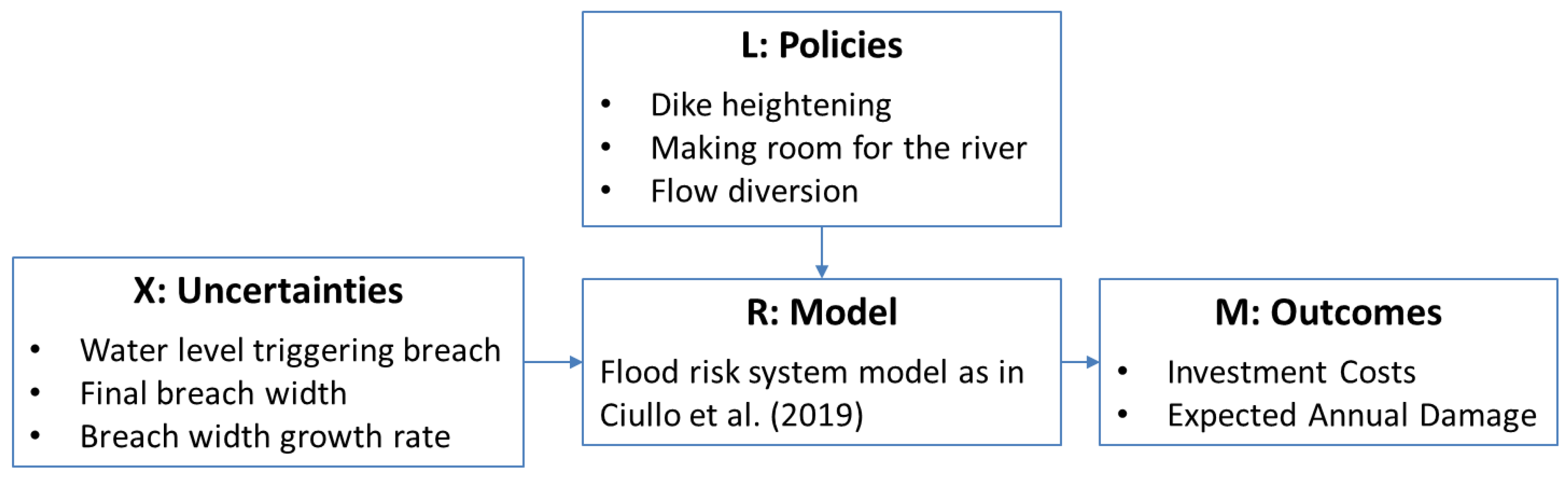
3.1. Policies (L)
3.2. Model Uncertainties (X)
3.3. Model Outcomes (M)
4. Method
- Striving for overall risk reduction and neglecting hydraulic interactions,
- ibid, but accounting for hydraulic interactions, and
- also accounting for risk distribution.
4.1. Policy Problem Formulations
4.2. Generating Alternatives
4.3. Evaluate Alternatives Under Uncertainty
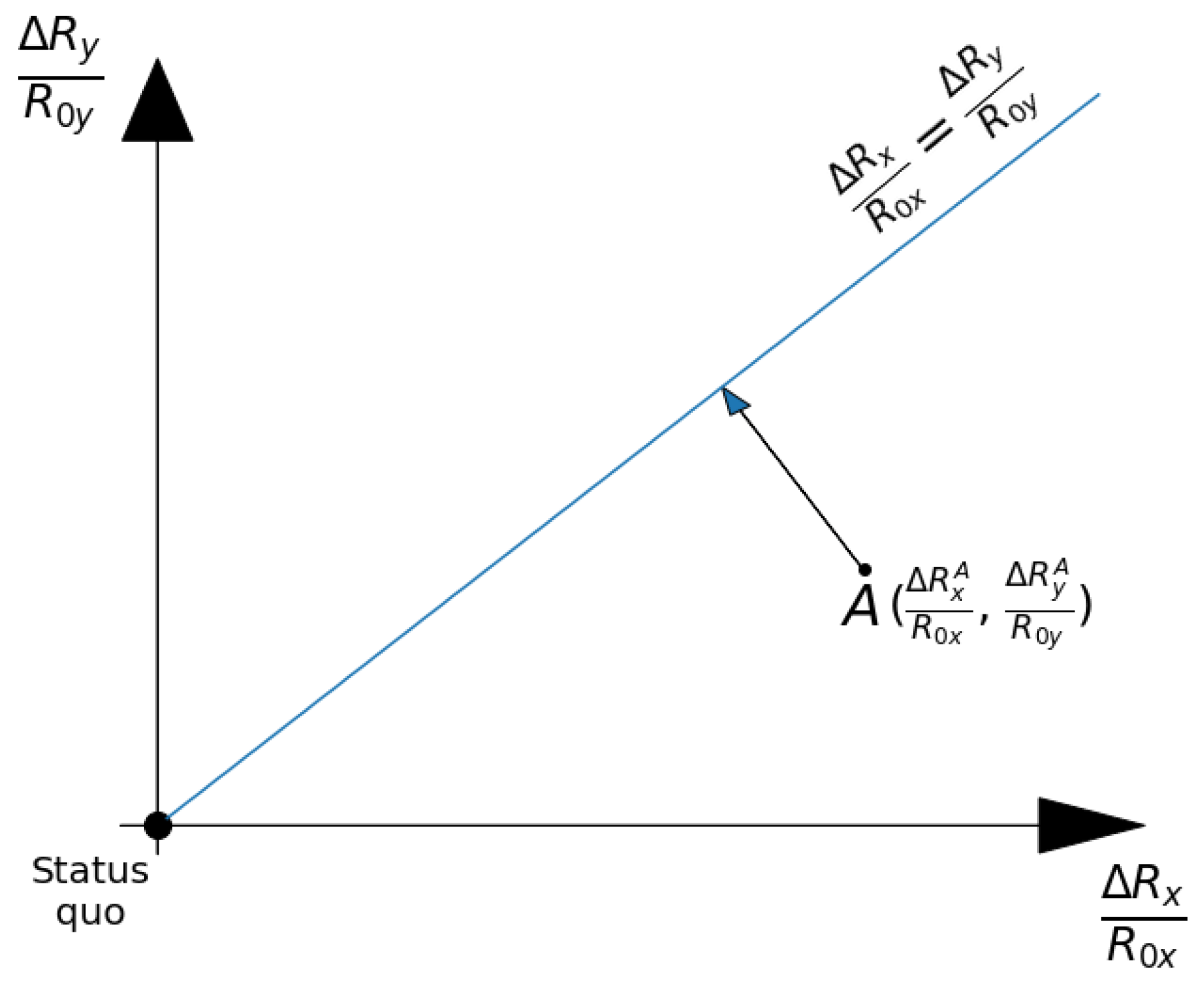
4.4. Evaluating Robustness Under Different Attitudes Towards Risk
5. Results
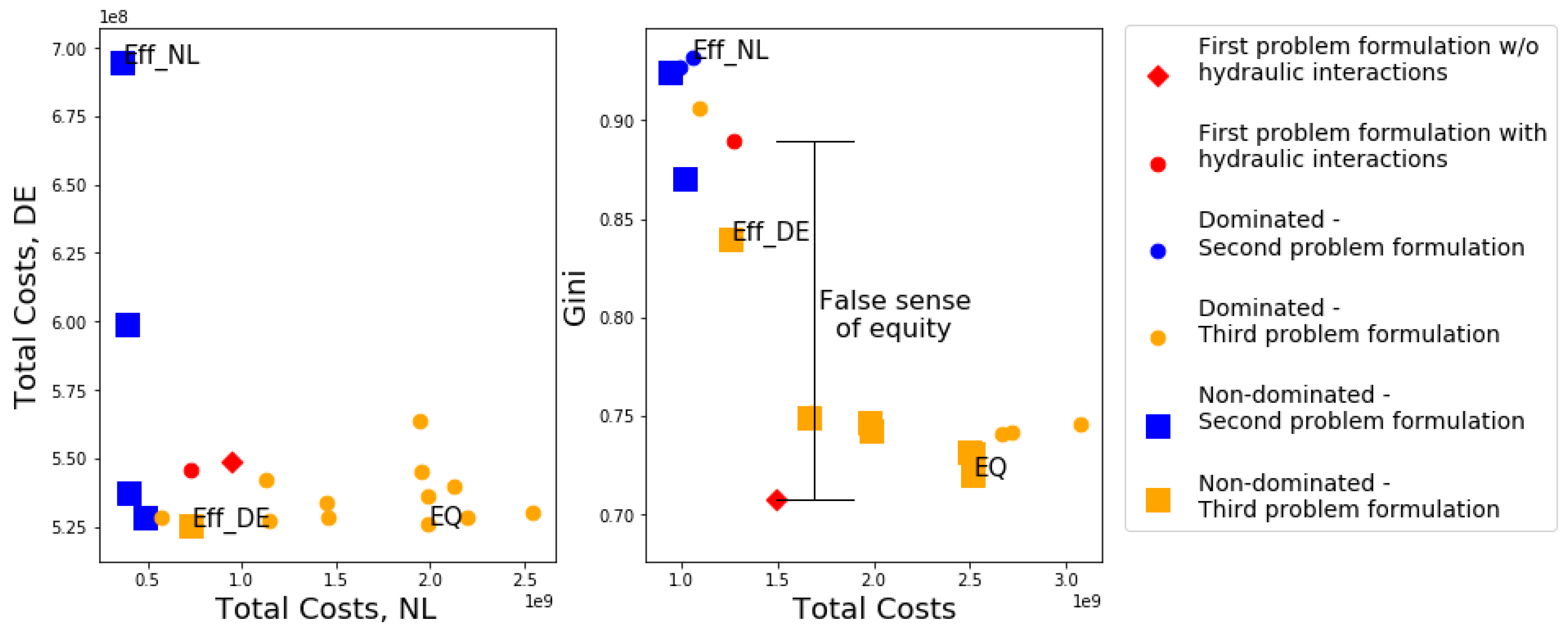
5.1. Generating Alternatives
5.2. Evaluating Robustness Under Different Attitudes Towards Risk
6. Discussion and Conclusions
Supplementary Materials
Author Contributions
Funding
Conflicts of Interest
References
- Di Baldassarre, G.; Castellarin, A.; Brath, A. Analysis of the effects of levee heightening on flood propagation : Example of the River Po, Italy. Hydrol. Sci. J. 2009, 54, 1007–1017. [Google Scholar] [CrossRef]
- Van Mierlo, M.C.L.; Vrouwenvelder, A.; Calle, E.O.F.; Vrijling, J.K.; Jonkman, S.N.; de Bruijn, K.M.; Weerts, A.H. Assessment of flood risk accounting for river system behaviour. Int. J. River Basin Manag. 2007, 5, 93–104. [Google Scholar] [CrossRef]
- De Bruijn, K.M.; Diermanse, F.L.M.; Van Der Doef, M.; Klijn, F. Hydrodynamic system behaviour: Its analysis and implications for flood risk management. E3S Web Conf. 2016, 7, 11001. [Google Scholar] [CrossRef]
- Vorogushyn, S.; Bates, P.D.; de Bruijn, K.; Castellarin, A.; Kreibich, H.; Priest, S.; Schröter, K.; Bagli, S.; Blöschl, G.; Domeneghetti, A. Evolutionary leap in large-scale flood risk assessment needed. Wiley Interdiscip. Rev. Water 2017, 5, 1–7. [Google Scholar] [CrossRef]
- Directive 2007/60/EC of the European Parliament and of the council of October 23, 2007 on the assessment and management of flood risks. Off. J. Eur. Union 2007, L288, 27–34.
- Orlandini, S.; Moretti, G.; Albertson, J.D. Evidence of an emerging levee failure mechanism causing disastrous floods in Italy. Water Resour. Res. 2015, 51, 7995–8011. [Google Scholar] [CrossRef]
- Hansson, S.O. Philosophical problems in cost-benefit analysis. Econ. Philos. 2007, 23, 163–183. [Google Scholar] [CrossRef]
- Kind, J.M. Economically efficient flood protection standards for the Netherlands. J. Flood Risk Manag. 2014, 7, 103–117. [Google Scholar] [CrossRef]
- Eijgenraam, C.; Brekelmans, R.; Hertog, D.D.E.N.; Roos, K. Optimal Strategies for Flood Prevention. Manag. Sci. 2017, 63, 1644–1656. [Google Scholar] [CrossRef]
- Brekelmans, R.; Den Hertog, D. Safe Dike Heights at Minimal Costs: The Nonhomogeneous Case. Oper. Res. 2012, 60, 1342–1355. [Google Scholar] [CrossRef][Green Version]
- Hayenhjelm, M. What Is a Fair Distribution of Risk. In Handbook of Risk Theory; Roeser, S., Hillerbrand, R., Sandin, P., Peterson, M., Eds.; Springer: Berlin, Germany, 2012. [Google Scholar] [CrossRef]
- Ciullo, A.; de Bruijn, K.M.; Kwakkel, J.H.; Klijn, F. Accounting for the uncertain effects of hydraulic interactions in optimising embankments heights: Proof of principle for the IJssel River. J. Flood Risk Manag. 2019. [Google Scholar] [CrossRef]
- Kasprzyk, J.R.; Nataraj, S.; Reed, P.M.; Lempert, R.J. Many objective robust decision making for complex environmental systems undergoing change. Environ. Model. Softw. 2013, 42, 55–71. [Google Scholar] [CrossRef]
- Coello Coello, C.; Lamont, G.B.; Van Veldhuizen, D.A. Evolutionary Algorithms for Solving Multiobjective Problems; Springer: Raleigh, NC, USA, 2007. [Google Scholar] [CrossRef]
- Silva, W.; Klijn, F.; Dijkman, J. Room for the Rhine Branches in the Netherlands. What the Research Has Taught Us; WL, Delft & RIZA: Arnhem, The Netherlands, 2001. [Google Scholar]
- Lammersen, R.; Kroekenstoel, D. Transboundary effects of extreme floods along the Rhine in Northrhine-Westfalia (Germany) and Gelderland (The Netherlands). In Floods, from Defence to Management; van Alphen, J., van Beek, E., Taal, M., Eds.; Taylor & Francis Group: London, UK, 2005; pp. 531–536. [Google Scholar]
- Lempert, R.J.; Popper, S.W.; Bankes, S.C. Shaping the Next One Hundred Years: New Methods for Quantitative, Long-Term Policy Analysis; MR-1626, RAND: Santa Monica, CA, USA, 2003. [Google Scholar]
- FLOODsite. Flood Risk Assessment and Flood Risk Management. An Introduction and Guidance Based on Experiences and Findings of FLOODsite (an EU-funded Integrated Project). Deltares Delft Hydraul. Available online: floodsite.net/html/partner_area/project_docs/T29_09_01_Guidance_Screen_Version_D29_1_v2_0_P02.pdf 140 (accessed on 29 November 2019).
- Van Schijndel, S.A.H. The planning kit, a decision making tool for the Rhine branches. In Proceedings of the 3rd International Symposium Flood Defence, Nijmegen, The Netherlands, 25–27 May 2005. [Google Scholar]
- De Grave, P.; Baarse, G. Kosten van Maatregelen: Informatie Ten Behoeve van Het Project Waterveiligheid 21e Eeuw (Deltares rep. 1204144-003). Available online: http://edepot.wur.nl/346748 (accessed on 29 November 2019).
- Kollat, J.B.; Reed, P.M. The value of online adaptive search: A performance comparison of NSGA-II, -NSGAII, and MOEA. In International Conference on Evolutionary Multi-Criterion Optimization (EMO 2005). Lecture Notes in Computer Science; Coello Coello, C., Aguirre, A., Zitzler, E., Eds.; Springer: Berlin, Germany, 2005; pp. 389–398. [Google Scholar]
- Hadka, D.; Reed, P. Borg: An Auto-Adaptive Many-Objective Evolutionary Computing Framework. Evol. Comput. 2013, 21, 231–259. [Google Scholar] [CrossRef] [PubMed]
- Zitzler, E.; Thiele, L.; Laumanns, M.; Fonseca, C.M.; da Fonseca, V.G. Performance assessment of multiobjective optimizers: An analysis and review. IEEE Trans. Evol. Comput. 2003, 7, 117–132. [Google Scholar] [CrossRef]
- Giuliani, M.; Castelletti, A. Is robustness really robust? How different definitions of robustness impact decision-making under climate change. Clim. Chang. 2016, 135, 409–424. [Google Scholar] [CrossRef]
- Kwakkel, J.H.; Eker, S.; Pruyt, E. How Robust is a Robust Policy? Comparing Alternative Robustness Metrics for Robust Decision-Making. In Robustness Analysis in Decision Aiding, Optimization, and Analytics; Springer: Singapore, 2016; pp. 221–237. [Google Scholar]
- McPhail, C.; Maier, H.R.; Kwakkel, J.H.; Giuliani, M.; Castelletti, A.; Westra, S. Robustness Metrics: How Are They Calculated, When Should They Be Used and Why Do They Give Different Results? Earth’s Futur. 2018, 6, 169–191. [Google Scholar] [CrossRef]
- Wald, A. Statistical Decision Functions; Chapman & Hall: London, UK; New York, NY, USA, 1950. [Google Scholar]
- Hurwicz, L. An Optimality Criterion for Decisionmaking under Ignorance. In Uncertain. Expect. Econ. Essays Honour GLS Shackle; Augustus M. Kelley: New York, NY, USA, 1953. [Google Scholar]
- Kwakkel, J.H. The Exploratory Modeling Workbench: An open source toolkit for exploratory modeling, scenario discovery, and (multi-objective) robust decision making. Environ. Model. Softw. 2017, 96, 239–250. [Google Scholar] [CrossRef]
- Gini, C. Measurement of Inequality nd Incomes. Econ. J. 1921, 31, 124–126. [Google Scholar] [CrossRef]


| Uncertainty | Water Level Triggering Failure | Final Breach Width | Breach Growth Rate |
|---|---|---|---|
| Values | Given by fragility curves at each location | Between 35 and 350 m | The final breach width can be reached in 1, 3, or 6 days |
| Water Level Triggering Failure | Final Breach Width | Breach Growth Dynamic |
|---|---|---|
| Water levels given by the fragility curves at a failure probability of 0.5 | The final breach width reaches a maximum width of 150 m | The final breach width is reached in 3 days |
| First Scenario | Second Scenario | Third Scenario | Minimin | Hurwicz = 0.8 | Hurwicz = 0.2 | Minimax ( = 0) | |
|---|---|---|---|---|---|---|---|
| Policy 1 | 3 | 5 | 3 | 3 | 3.4 | 4.6 | 5 |
| Policy 2 | 9 | 2 | 6 | 2 | 3.4 | 7.6 | 9 |
| Policy 3 | 7 | 1 | 11 | 1 | 3 | 9 | 11 |
© 2019 by the authors. Licensee MDPI, Basel, Switzerland. This article is an open access article distributed under the terms and conditions of the Creative Commons Attribution (CC BY) license (http://creativecommons.org/licenses/by/4.0/).
Share and Cite
Ciullo, A.; De Bruijn, K.M.; Kwakkel, J.H.; Klijn, F. Systemic Flood Risk Management: The Challenge of Accounting for Hydraulic Interactions. Water 2019, 11, 2530. https://doi.org/10.3390/w11122530
Ciullo A, De Bruijn KM, Kwakkel JH, Klijn F. Systemic Flood Risk Management: The Challenge of Accounting for Hydraulic Interactions. Water. 2019; 11(12):2530. https://doi.org/10.3390/w11122530
Chicago/Turabian StyleCiullo, Alessio, Karin M. De Bruijn, Jan H. Kwakkel, and Frans Klijn. 2019. "Systemic Flood Risk Management: The Challenge of Accounting for Hydraulic Interactions" Water 11, no. 12: 2530. https://doi.org/10.3390/w11122530
APA StyleCiullo, A., De Bruijn, K. M., Kwakkel, J. H., & Klijn, F. (2019). Systemic Flood Risk Management: The Challenge of Accounting for Hydraulic Interactions. Water, 11(12), 2530. https://doi.org/10.3390/w11122530