Article

Measuring Surface Velocity of Water Flow by Dense Optical Flow Method

1
College of Mechanical & Electronic Engineering, Northwest A & F University, Yangling 712100, China
2
College of Water Resources and Architectural Engineering, Northwest A & F University, Yangling 712100, China
*
Author to whom correspondence should be addressed.
Water 2019, 11(11), 2320; https://doi.org/10.3390/w11112320
Submission received: 21 September 2019 / Revised: 31 October 2019 / Accepted: 1 November 2019 / Published: 6 November 2019
(This article belongs to the Section Hydraulics and Hydrodynamics)

Abstract

:
Recent advances in video processing technology have provided a new approach to measuring the surface velocity of water flow (SVWF). However, most of the previous researches using video processing technology depended on tracers for target tracing, requiring spraying tracers in the measurement process. These methods are not convenient for velocity measurement. In this study, a dense optical flow method (Farneback optical flow method) was used to process the water flow video to get the estimated SVWFs. The estimated SVWFs were verified by the actual SVWFs measured by a portable propeller velocimeter. The regression analyses between the estimated SVWFs and the measured SVWFs were conducted. The coefficient of determinations (R2) of the estimated and the measured SVWFs in different test regions are between 0.81 and 0.85. The average relative errors of the estimated and the measured SVWFs in all test regions are no more than 6.5%. The results indicate that the method had a good accuracy in estimating the SVWF and is a feasible and promising approach to analyzing the surface velocity distribution of water flow.

1. Introduction

Velocity measurement of water flow is an important task in hydrological monitoring [1,2,3]. The commonly used methods are using contact measurement instruments, such as propeller velocimeters and electromagnetic flow velocimeters. These devices can directly measure multi-point velocities by completely submerging in water but are susceptible to damage [4]. Ultrasonic Doppler velocimetry uses a non-contact measurement device for measuring flow velocity [5,6,7]. It utilizes the Doppler effect of the ultrasonic wave to measure the frequency between the incident wave and the reflected wave to obtain the flow velocity, but it can’t reflect the velocity distribution of water flow, and the equipment installation is complicated [8]. Therefore, it would be valuable to develop a new convenient and easy-to-use flow velocity measuring method.
With the development of image and video processing technologies, flow velocity measurement methods based on video processing techniques have been proposed. Fujita et al. [9,10] proposed a high-precision surface velocity of water flow (SVWF) measuring method known as the particle imaging velocimetry (PIV) method. This method calculated the SVWF by measuring the displacement of tracer particles within a short time. Jodeau et al. [11] used large scale particle image velocity (LS-PIV) method to measure the SVWF in a mountain stream during high flow conditions due to a reservoir release, and the SVWF was converted into depth-averaged velocities to calculating discharges. Han et al. [12] employed micro-PIV technique to measure the water flow rates for three types of T-shaped micro-channel, obtaining the velocity distributions on the cross section of the microchannels. PIV method is suitable for analyzing complex flow velocity field distributions [13,14]. However, it requires spraying of tracing particles continuously, and it also has strict requirements in terms of the shape, size, and scattering rate of the tracer objects [15,16,17,18]. Jeanbourquin et al. [19] took the floating wastes on the sewer water surface as tracers, using PIV method to estimate sewer flow velocity. However, the method has obvious limitations in the absence of floating matter.
Dense optical flow (DOF) method is a tracer-independent object motion measurement method based on video processing techniques [20,21]. It is a point-by-point method for deriving the moving direction and velocity of targets from analyzing the displacement of these targets in two successive video images [22,23,24,25]. A few studies based on the DOF method have already been conducted in velocity measurement field. Wu et al. [26] applied the DOF method to estimate the red blood cell (RBC) velocity based on acquired capillary videos, indicating this method has the potential to provide more specific and detailed information of RBC velocity in microcirculation. Zheng et al. [27] developed a measurement method for the acquisition of the thermal smoke flow velocity profiles based on the optical flow method in fire building experiments, using the traditional point measurement and simulation results to verify the feasibility of the optical-based method. The results indicated that the optical flow method was a feasible measurement method for fire smoke flow fields. However, few researches on the measurement of surface velocity of water flow (SVWF) by DOF method have been found.
In this study, we aim to explore the feasibility of measuring SVWF by DOF method. We recorded the channel flow videos by a camera, and processed the video by DOF method to obtain the estimated flow surface velocity field. A portable propeller velocimeter was used to obtain the actual SVWF. The regression analysis of estimated and actual velocities was carried out to verify the feasibility and accuracy of the method.

2. Methodology

2.1. Principle Analysis of DOF Method

DOF method is one of object motion estimation methods based on video processing techniques. It has two hypotheses: The gray level observed at any object point remains unchanged for a short time (gray level invariant hypothesis); the adjacent points in the image plane move in a similar way (velocity smoothing constraints) [28,29,30]. The calculation principle is as follows.
As shown in Figure 1, we suppose that each small grid represents a pixel. The pixel P in the image represents a tracing target point. It moves to pixel P’ within the time interval (∆t) of two successive images.
Using symbols I(xp, yp, t) to represent the gray value of P(xp, yp) at time t, the gray value of P’(xp + ∆x, yp + ∆y) at time t + ∆t can be expressed as I(xp + ∆x, yp + ∆y, t + ∆t). According to the above gray scale invariant hypothesis:
I ( x p , y p , t ) = I ( x p + Δ x , y p + Δ y , t + Δ t )
Using the Taylor series expansion to expand Equation (1):
I ( x p + Δ x , y p + Δ y , t + Δ t ) = I ( x p , y p , t ) + I x Δ x + I y Δ y + I t Δ t + ε
Applying equation (1) and ignoring the higher order terms (ε) in Equation (2), the following equation can be obtained:
I x Δ x Δ t + I y Δ y Δ t + I t = 0
Using u and v to represent the component of the optical flow vector along the X and Y directions respectively:
u = Δ x / Δ t
v = Δ y / Δ t
According to Equations (4) and (5), Equation (3) can be turned into:
I x u + I y v + I t = 0
Equation (6) is the fundamental equation of optical flow method. There are many methods to calculate DOF. The Farneback optical flow method (FOFM) based on gray level invariant hypothesis is more accurate than other optical flow methods [31,32,33]. In this study, the FOFM was used to solve the problem.
For a small image neighborhood area (with yellow marks in Figure 1), the gray level function F(x, y) of the pixel X = (x y)T can be approximately expressed by a binary quadratic polynomial:
F ( x , y ) = a 0 + a 1 x + a 2 y + a 3 x 2 + a 4 y 2 + a 5 x y
Equation (7) can be written in matrix form.
F ( X ) = X T A X + b T X + c
where:
c = a 0
b = ( a 1 a 2 ) T
A = ( a 3 a 5 / 2 a 5 / 2 a 4 )
The gray value of the pixels X at time t is:
F t ( X ) = X T A t X + b t T X + c t
After a short time interval ∆t, the displacement of X is ∆X (∆x, ∆y), so the gray value of (X +X) is:
F t + Δ t ( X + Δ X ) = ( X + Δ X ) T A t + Δ t ( X + Δ X ) + b T t + Δ t ( X + Δ X ) + c t + Δ t
Turning Equation (13) into:
F t + Δ t ( X + Δ X ) = X T A t + Δ t X + ( b t + Δ t + 2 A t + Δ t Δ X ) T X + Δ X T A t + Δ t Δ X + b T t + Δ t Δ X + c t + Δ t
According to the hypothesis of gray level invariant hypothesis:
F t ( X ) = F t + Δ t ( X + Δ X )
Equating the coefficients of Equations (12) and (14):
A t = A t + Δ t
b t = b t + Δ t + 2 A t + Δ t Δ X
c t = c t + Δ t + Δ X T A t + Δ t Δ X + b T t + Δ t Δ X
Turning Equation (17) into:
A t + Δ t Δ X = 1 / 2 ( b t + Δ t b t )
Ideally At+t and At should be equal but in practice we have to make the following approximation:
A M = 1 / 2   ( A t +   A t + Δ t )
Introducing:
Δ b = 1 / 2   ( b t + Δ t b t )
Using AM to r At+t, the Equation (19) can be turned into:
A M Δ X = Δ b
To reduce the influence of noise, the error function e(X) of the neighborhood area (D) of the target pixel is constructed. The displacement (∆X) of the target point during the corresponding time is determined by minimizing the error function e(X), from which the velocity of the pixel is deduced.
e ( X ) = Δ D D ω ( Δ D ) A M ( X + Δ D ) Δ X Δ b ( X + Δ D ) 2
where ωD) the Gauss weighting function in neighborhood area D. In this study, we used a 5 × 5 pixels neighborhood area. The ωD) is used to reflect the influence degree of each point in the neighborhood area. The closer each pixel is to the target pixel in the neighborhood area, the greater the value of the Gauss weighting function is.

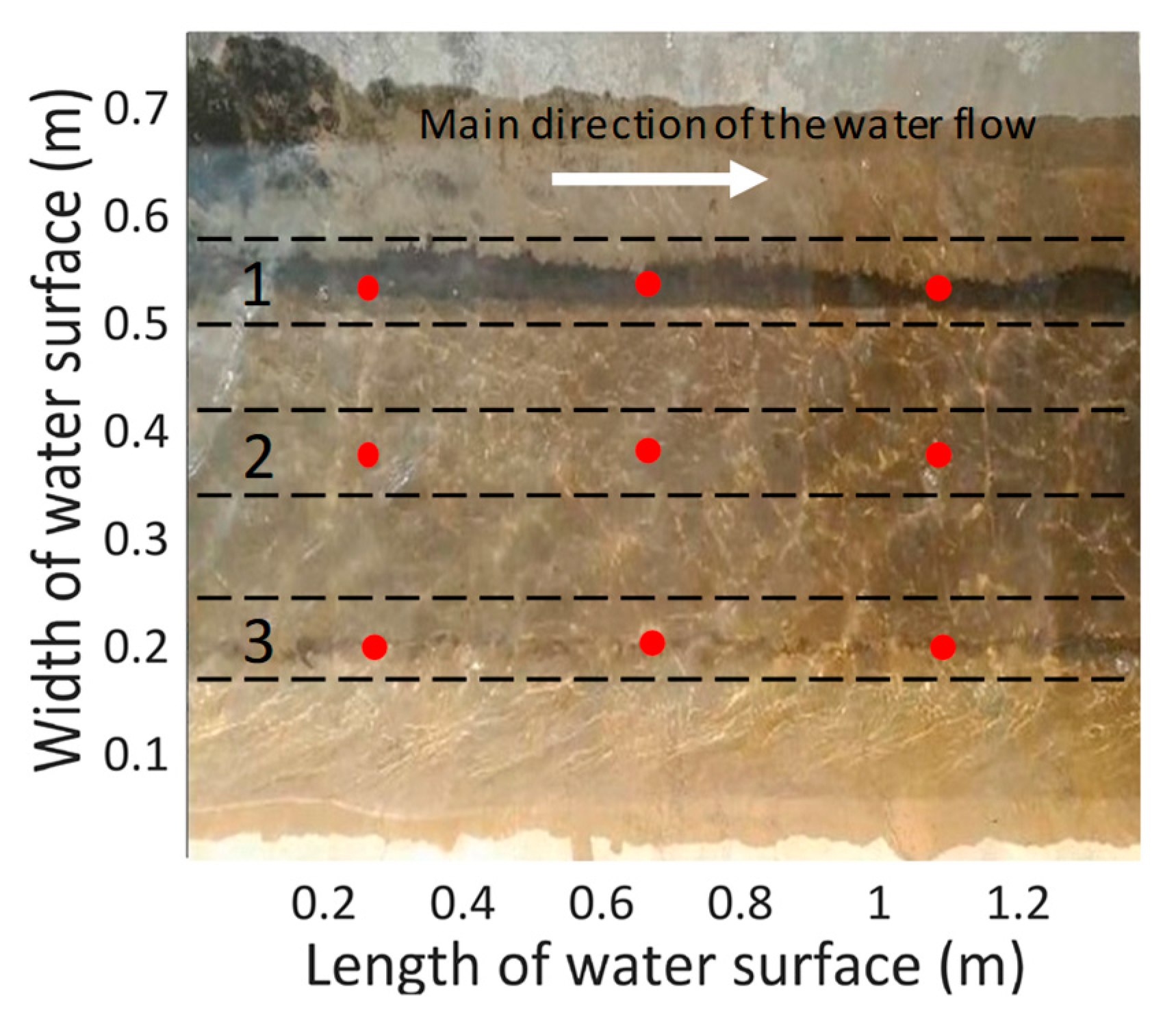
2.2. Experiment Design

The flow velocity measurement experiments were carried out in a standard trapezoidal channel (15 m in length, 150 cm in upper width, 30 cm in bottom width, and 60 cm in depth) in the experimental irrigation station of Northwest A & F University, Yangling, Shaanxi Province, China. The optical flow method estimates the flow velocity by identifying the movement of the ripples. If the water surface is shaded, the ripples change dramatically from the bright area to the shaded area, which cannot be accurately identified. Therefore, the experiment was carried out under the condition of good light and no shadows on the water surface.

2.2.1. Experiment Preparatory Work

The flow video materials were recorded by a camera. We fixed the camera on a tripod. The lens was set to be parallel to the water flow surface and one meter away from the water surface. The image captured by camera needed to be calibrated to obtain the relationship between the actual distance and the pixels [34,35,36,37]. A rectangular box of 20 cm × 25 cm was used to calibrate. After calibration, when the lens was one meter away from the water surface, the actual distance represented by one pixel was 2.13 mm.

2.2.2. Actual Flow Velocity Measurement and Video Acquisition

We carried out 20 tests. For each test, we made the channel pass through different discharges and keep the flow stable. The types of the flow were subcritical flow. Three typical regions on the water surface were selected to measure their SVWF and each region contained three measurement points, as shown in Figure 2. The width of each typical region was 6.5 cm, and the length was 136 cm (the length of the channel within the video recording range). In velocity measurement, the SVWF in the main direction (the direction parallel to the channel bank) was the most concerned. The actual SVWF in the main direction was measured by an LS300-A portable propeller velocimeter (Weifang Huayu Hydrological Science and Technology Co., Ltd, Weifang, China) with an accuracy of 0.001 m/s. The diameter of the propeller was 15 mm. The propeller was put into the water 1 to 2 cm to measure the SVWF. According to the ideal relationship between channel depth and flow rate, the shallow flow velocity is very close to the surface velocity. Thus, we assumed that the velocity measured by the velocimeter was the surface velocity. After the velocities of nine measurement points were measured, the velocimeter was moved out of the recording range of the camera to get the flow video material (at least 10 s) without interference. We repeated the velocity measurement and video acquisition five times for each test. The average of five measured SVWFs of each point was regarded as the actual SVWF of that point. The average of the measured SVWF of three target points in a region was considered as the actual SVWF of that region.

2.2.3. Video Processing

For each test, we intercepted a 5 s (30 frames per second) video clip from corresponding non-interference recorded video. These video clips were processed with the FOFM for SVWF estimation. The original image resolutions of captured videos were 1080 × 1920 pixels. To improve the computational efficiency and stability of the results, the image resolutions were converted to 360 × 640 pixels while calibrating and calculating optical flow. The video processing was executed in the MATLAB environment on an computer (i7-4790K CPU @ 4.00 GHz) (ASUS Computer (Shanghai) Co., Ltd., Shanghai, China). The processing algorithm was called the Computer Vision System Toolbox of MATLAB 2018b.

3. Results and Discussion

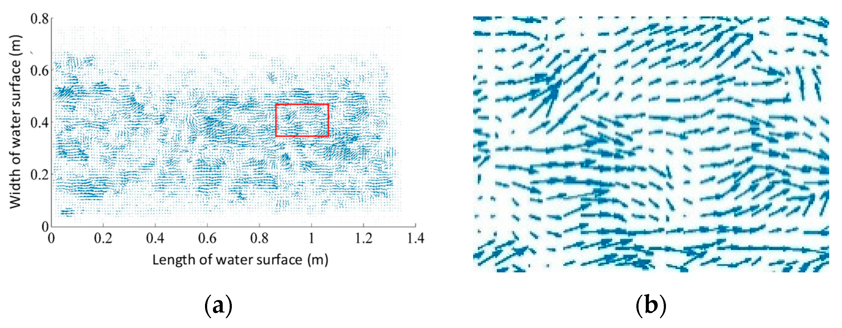
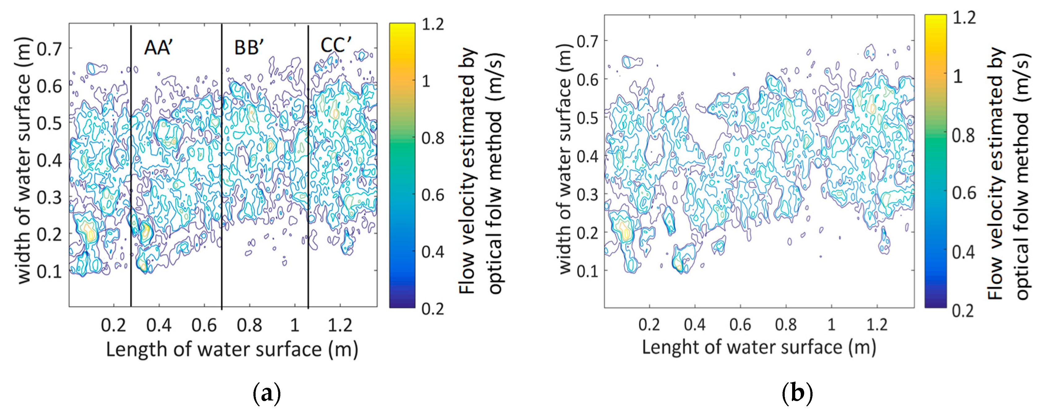
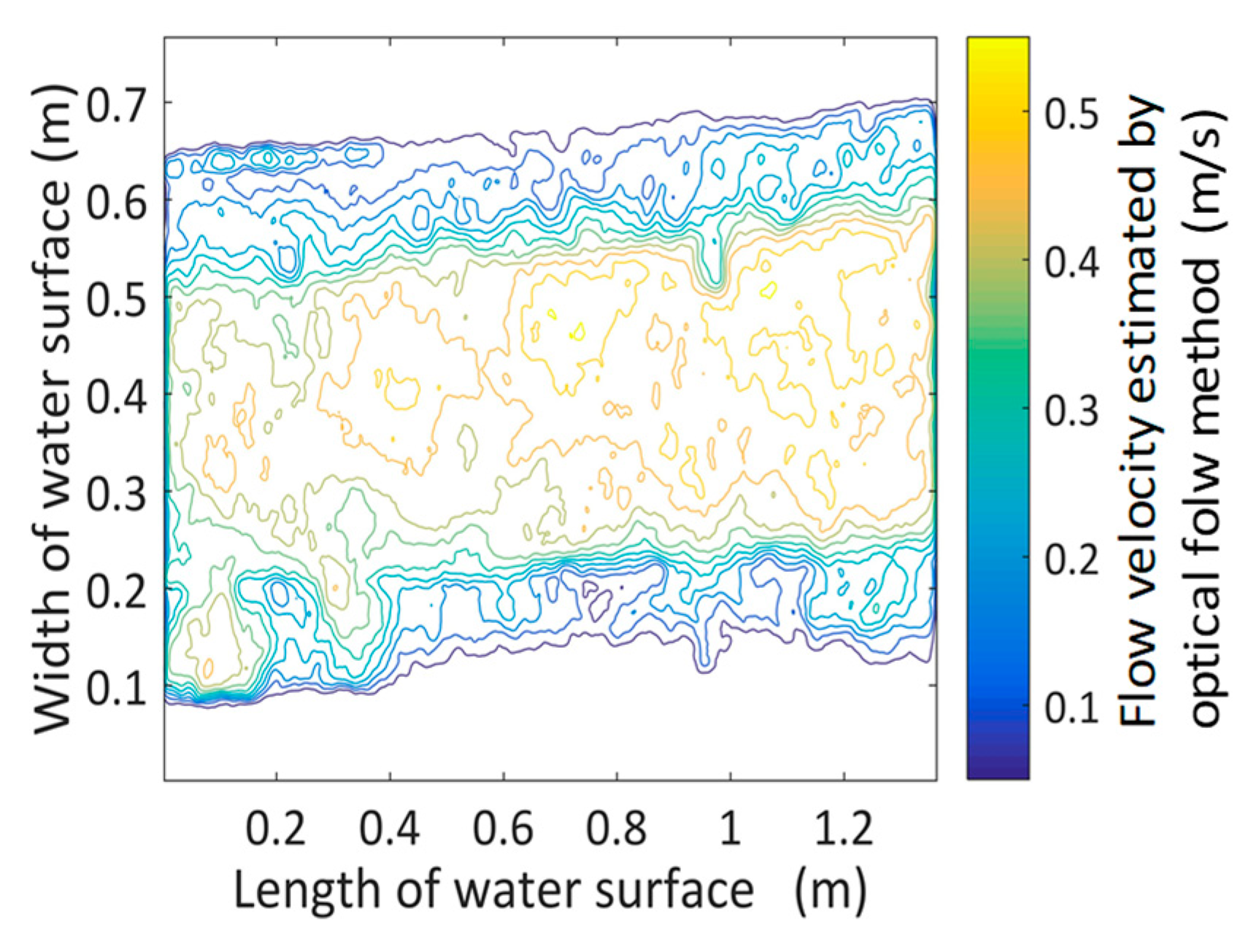
3.1. Water Flow Surface Velocity Field

The pixel displacement of the target point in two consecutive frames can be obtained by FOFM. According to the relationship between the pixel and the actual distance (2.13 mm/pix), the actual displacement of the target point can be deduced. The SVWF of the target point in the time interval of two successive frames can be calculated. On the test computer, it took 0.09 s to derive the vector SVWF distribution map from two frames of image using FOFM. The vector SVWF field is shown in Figure 3a.
As can be seen from Figure 3b (the local enlargement diagram of the area marked by the red box in Figure 3a), the direction of SVWF is not completely parallel to the channel bank. In this study, we mainly focused on the SVWF in the main direction (vm). To obtain the value of vm, we decomposed the vector velocity into the velocity component in the main direction and the velocity component perpendicular to the main direction (vp). The surface velocities of water flow mentioned below refer to the velocities along the main direction.

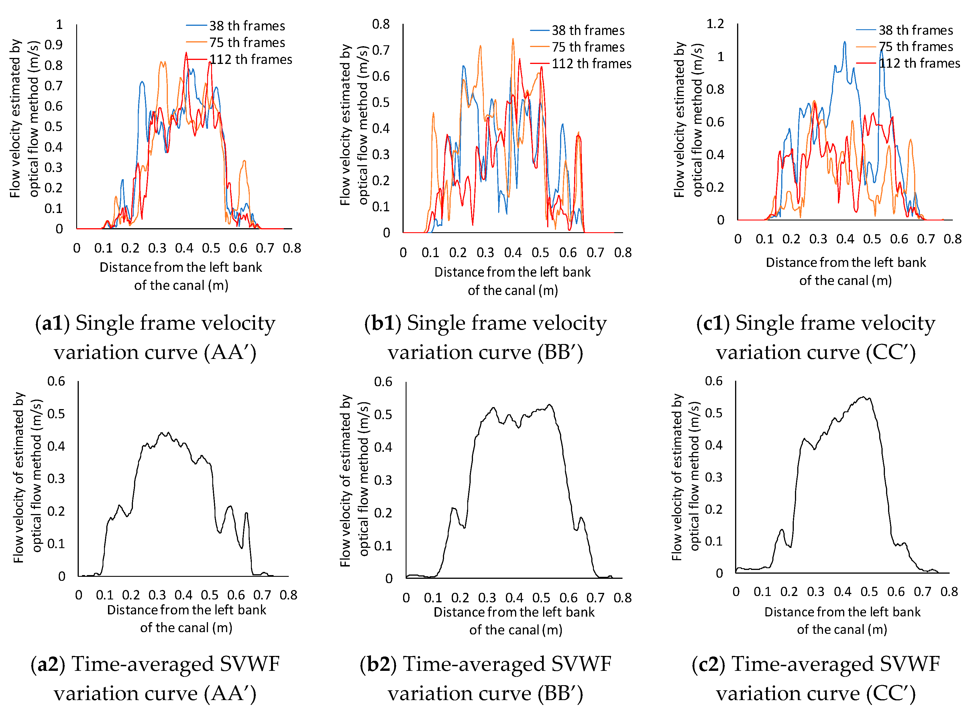
3.2. Time-Averaged SVWF

Using FOFM, a velocity field map can be obtained according to two successive frames of images. It was stipulated that the velocity field map derived from the first frame and the second frame images was called the velocity field map of the 1st frame, and the velocity field map derived from the second frame and the third frame images was called the velocity field of the 2nd frame, and so on.
Because of the complex flow on the water surface and the dramatic variation of water surface ripple, the estimated SVWF fields of different video frames were different (Figure 4). Figure 5 shows the relationship between the SVWF of each target point on three straight lines (AA’, BB’, CC’ in Figure 3) and its distance from the left bank of the channel of the selected three typical frame images (38th frame, 75th frame and 112th frame). It could be seen from the graphs (Figure 5a1–c1) that although the variation trend curves of SVWF was roughly in line with the distribution characteristic of the SVWF in the channel, they fluctuated greatly. The consistency of peaks and troughs of SVWF variation trend curves of the same straight line in different frames was unfavorable. However, after average-processing of the SVWFs obtained from 150 frames of images, the SVWF variation trend curves tended to be stable (Figure 5a2–c2). In order to obtain relative stable velocity estimation, we averaged SVWFs of all frames of a video clip in each test. The time-averaged SVWF (va) distribution is shown in Figure 6.

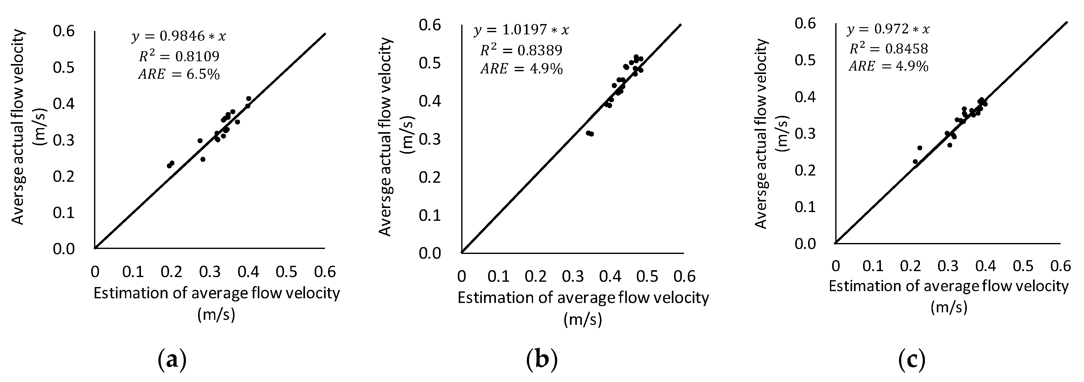
3.3. Velocity Estimation and Error Analysis

In one test, five measurements were repeated and five video clips were obtained within the measurement interval. Taking region 1 (Figure 2) as an example, the average value of all va in region 1 of five videos was taken as the estimated average SVWF (hereinafter referred to as the estimated SVWF). According to the aforementioned method, the estimated velocities in each region were obtained. Then regression analysis of average actual SVWFs (measured by the velocimeter) and the estimated SVWFs were made to evaluate the accuracy and reliability of the FOFM (Figure 7). The regression formulas are listed in Table 1.
As shown in Figure 7, the estimated SVWFs of regions 1 (Figure 7a) and 3 (Figure 7c) ranged from 0.2 to 0.4 m/s, and the estimated SVWFs of region 2 (Figure 7b) ranged from 0.3 to 0.5 m/s. The distribution ranges of estimated velocity were approximately the same as the measured velocity distribution ranges. The correlation coefficients (R2) between estimated SVWFs and average measured SVWFs in regions 1, 2, and 3 were 0.8109, 0.8389, and 0.8458, respectively. The R2 of each region was greater than 0.8, which indicated that the estimated velocity in each region had a strong correlation with the actual average velocity. The average relative errors (ARE) of estimated SVWFs and measured SVWFs in regions 1, 2, and 3 were 6.5%, 4.9%, and 4.9%, respectively. The results showed that the FOFM had a good accuracy in estimating the SVWF of each water surface region. Furthermore, it meant the method adopted was a feasible and promising approach to analyzing the SVWF.

4. Conclusions

In this study, the FOFM was introduced into the measurement of SVWF. The surface vector velocity field of water flow was obtained by this method. In velocity measurement, the SVWF in the main direction is the most concerned, thus the estimated vector velocities were transformed into the velocity along the main direction of the water flow. Because the velocity field of different frames changed dramatically, the velocity field of any frame image could not reflect the average velocity distribution of the flow surface in the time interval. Therefore, the estimated SVWFs were averaged over time, and the time-averaged SVWFs were obtained.
Finally, the regression analysis between the estimated SVWFs and the measured SVWFs were conducted, and the results showed that the estimated velocity could well reflect the actual velocity. At the same time, the performance of the estimated velocity in three regions of the flow surface was evaluated. The results showed that the method had good estimation effect in different regions of the flow surface. The adopted DOF method (FOFM) was concluded to be a better and more promising option in measuring SVWF and estimating the flow field distribution on the surface of water flow approximately.
Note that, although the FOFM is a simple and easy-to-use method, which can obtain the SVWF without continuously spraying tracers, the performance of the method is affected by the distribution of light on the surface of the flow. The FOFM is based on gray level invariant hypothesis. Once shadow appears in some areas of the image, the gray levels of the target points going through unshaded area to shaded area will change, obviously. It will have mismatches while using the FOFM to track these target points. The mismatches of these target points will affect the calculation of velocity. If there are shadows on the water surface in some areas during video recording, it may affect the calculation of optical flow and lead to larger errors in the estimation results. The video used in this study was recorded in clear weather and clear water flow, and the influence of shadows on the water surface on this method needs further researches.

Author Contributions

Research conceptualization, H.W. and X.M.; data curation, H.W., R.Z. and X.M.; methodology, H.W., R.Z. and X.G.; writing—original draft, H.W.; writing—review & editing, X.M.

Funding

This research was financially supported by the 13th Five-Year Plan for the Key Project of Research and Development (grant No. 2016YFC0400203) and the National Key R & D Program of China (No. 2017YFC0403202).

Conflicts of Interest

The authors declare no conflicts of interest.

References

  1. Siebert, S.; Burke, J.; Faures, J.M.; Frenken, K.; Portmann, F.T. Groundwater Use for Irrigation–A Global Inventory. J. Hydrol. Earth Syst. Sci. Discuss. 2010, 7. [Google Scholar] [CrossRef]
  2. Pereira, L.S.; Oweis, T.; Zairi, A. Irrigation management under water scarcity. J. Agric. Water Manag. 2002, 57, 175–206. [Google Scholar] [CrossRef]
  3. Kim, Y.; Evans, R.G.; Iversen, W.M. Remote Sensing and Control of an Irrigation System Using a Distributed Wireless Sensor Network. J. IEEE Trans. Instrum. Meas. 2008, 57, 1379–1387. [Google Scholar]
  4. Aricò, C.; Corato, G.; Tucciarelli, T. Discharge estimation in open channels by means of water level hydrograph analysis. J. Hydraul. Res. 2010, 48, 612–619. [Google Scholar] [CrossRef]
  5. Kawanisi, K.; Razaz, M.; Ishikawa, K. Continuous measurements of flow rate in a shallow gravel-bed river by a new acoustic system. J. Water Resour. Res. 2012, 48, 5547. [Google Scholar] [CrossRef]
  6. Katakura, K.; Alain, P. Ultrasonic measurement method for transversal component of water flow velocity. In Proceedings of the International Symposium on Underwater Technology, Tokyo, Japan, 16–19 April 2002; pp. 45–48. [Google Scholar]
  7. Yoo, M.W.; Kim, Y.D.; Lyu, S. Flowrate and Velocity Measurement in Nakdong River Using ADCP. In Advances in Water Resources and Hydraulic Engineering; Springer: Berlin/Heidelberg, Germany, 2009; pp. 1946–1949. [Google Scholar]
  8. Bradley, A.A.; Kruger, A.; Meselhe, E.A. Flow measurement in streams using video imagery. J. Water Resour. Res. 1999, 38, 51. [Google Scholar] [CrossRef]
  9. Fujita, I.; Muste, M.; Kruger, A. Large-scale particle image velocimetry for flow analysis in hydraulic engineering applications. J. Hydraul. Res. 1998, 36, 397–414. [Google Scholar] [CrossRef]
  10. Fujita, I.; Aya, S. Refinement of LS-PIV Technique for Monitoring River Surface Flows. J. Water Res. 2000. [Google Scholar] [CrossRef]
  11. Jodeau, M.; Hauet, A.; Paquier, A.; Le Coz, J.; Dramais, G. Application and evaluation of LS-PIV technique for the monitoring of river surface velocities in high flow conditions. J. Flow Meas. Instrum. 2008, 19, 117–127. [Google Scholar] [CrossRef] [Green Version]
  12. Han, W.; Wang, H. Measurements of water flow rates for T-shaped microchannels based on the quasi-three-dimensional velocities. J. Meas. Sci. Technol. 2012, 23, 055301. [Google Scholar] [CrossRef]
  13. Fujita, I.; Tsubaki, R. A Novel Free-Surface Velocity Measurement Method Using Spatio-Temporal Images. J. Hydraul. Meas. Exp. Methods 2002. [Google Scholar] [CrossRef]
  14. Gunawan, B.; Sun, X.; Sterling, M. The application of LS-PIV to a small irregular river for inbank and overbank flows. J. Flow Meas. Instrum. 2012, 24, 1–12. [Google Scholar] [CrossRef] [Green Version]
  15. Bin Asad, S.M.S.; Lundström, T.S.; Andersson, A.G.; Hellström, J.G.I.; Leonardsson, K. Wall Shear Stress Measurement on Curve Objects with PIV in Connection to Benthic Fauna in Regulated Rivers. J. Water 2019, 11, 650. [Google Scholar] [CrossRef]
  16. Fang, S.Q.; Chen, Y.P.; Xu, Z.S.; Otoo, E.; Lu, S.Q. An Improved Integral Model for a Non-Buoyant Turbulent Jet in Wave Environment. J. Water 2019, 11, 765. [Google Scholar] [CrossRef]
  17. Bai, R.; Zhu, D.; Chen, H.; Li, D. Laboratory Study of Secondary Flow in an Open Channel Bend by Using PIV. J. Water 2019, 11, 659. [Google Scholar] [CrossRef]
  18. Scarano, F. Tomographic PIV: principles and practice. J. Meas. Sci. Technol. 2013, 24, 012001. [Google Scholar] [CrossRef]
  19. Jeanbourquin, D.; Sage, D.; Nguyen, L. Flow measurements in sewers based on image analysis: automatic flow velocity algorithm. J. Water Sci. Technol. A J. Int. Assoc. Water Pollut. Res. 2011, 64, 1108–1114. [Google Scholar] [CrossRef]
  20. Milan, S.; Roger, B.; Vaclav, H. Image Processing, Analysis, and Machine Vision; Chapman & Hall Computing: Boca Raton, FL, USA, 1993. [Google Scholar]
  21. Xiaoping, H.; Ahuja, N. Motion and structure estimation using long sequence motion models. J. Image Vis. Comput. 1993, 11, 549–569. [Google Scholar] [CrossRef]
  22. Zach, C.; Pock, T.; Bischof, H. A Duality Based Approach for Realtime TV-L1 Optical Flow. J. DAGM 2007, 214–223. [Google Scholar] [CrossRef]
  23. Weinzaepfel, P.; Revaud, J.; Harchaoui, Z.; Schmid, C. DeepFlow: Large Displacement Optical Flow with Deep Matching. In Proceedings of the 2013 IEEE International Conference on Computer Vision, Sydney, Australia, 1–8 December 2013; pp. 1385–1392. [Google Scholar]
  24. Chiuso, A.; Favaro, P.; Jin, H.; Soatto, S. Structure from motion causally integrated over time. J. IEEE Trans. Pattern Anal. Mach. Intell. 2002, 24, 523–535. [Google Scholar] [CrossRef]
  25. Pei, S.C.; Lin, G.L. Vehicle-type motion estimation by the fusion of image point and line features. J. Pattern Recognit. Soc. 1998, 31, 333–344. [Google Scholar]
  26. Wu, C.C.; Zhang, G.; Huang, T.C.; Lin, K.P. Red blood cell velocity measurements of complete capillary in finger nail-fold using optical flow estimation. J. Microvasc. Res. 2009, 78, 319–324. [Google Scholar] [CrossRef] [PubMed]
  27. Zheng, Y.; Zhou, X.D.; Ye, K.; Liu, H.; Cao, B.; Huang, Y.B.; Ni, Y.; Yang, L.Z. A two-dimension velocity field measurement method for the thermal smoke basing on the optical flow technology. J. Flow Meas. Instrum. 2019, 70, 201637. [Google Scholar] [CrossRef]
  28. Horn, B.K.P.; Schunck, B.G. Determining optical flow. J. Artif. Intell. 1981, 17, 185–203. [Google Scholar] [CrossRef] [Green Version]
  29. Kearney, J.K.; Thompson, W.B. Bounding Constraint Propagation for Optical Flow Estimation. In Motion Understanding; Springer: Boston, MA, USA, 1988. [Google Scholar]
  30. Ke, R.; Li, Z.; Tang, J.; Wang, Y. Real-Time Traffic Flow Parameter Estimation from UAV Video Based on Ensemble Classifier and Optical Flow. J. IEEE Trans. Intell. Transp. Syst. 2018, 1–11. [Google Scholar] [CrossRef]
  31. Farneback, G. Fast and accurate motion estimation using orientation. In Proceedings of the 15th IAPR International Conference on Pattern Recognition, Barcelona, Spain, 3–8 September 2000. [Google Scholar]
  32. Farneback, G. Two-Frame Motion Estimation Based on Polynomial Expansion. J. Lect. Notes Comput. Sci. 2003, 363–370. [Google Scholar] [CrossRef] [Green Version]
  33. Farneback, G. Very high accuracy velocity estimation using orientation tensors, parametric motion, and simultaneous segmentation of the motion field. In Proceedings of the IEEE International Conference on Computer Vision, Cambridge, MA, USA, 6 August 2002. [Google Scholar]
  34. Zhang, Z. Flexible camera calibration by viewing a plane from unknown orientations. In Proceedings of the Seventh IEEE International Conference on Computer Vision, Kerkyra, Greece, 20–27 September 1999. [Google Scholar]
  35. Geiger, A.; Moosmann, F.; Car, O.; Schuster, B. Automatic camera and range sensor calibration using a single shot. In Proceedings of the IEEE International Conference on Robotics and Automation, St. Paul, MN, USA, 14–18 May 2012; pp. 3936–3943. [Google Scholar]
  36. Hoang, V.D.; Danilo, C.H.; Jo, K.H. Simple and Efficient Method for Calibration of a Camera and 2D Laser Rangefinder. In Lecture Notes in Computer Science; Springer: Berlin, Germany, 2014; pp. 561–570. [Google Scholar]
  37. Dong, W.; Isler, V. A Novel Method for Extrinsic Calibration of a 2-D Laser-Rangefinder and a Camera. IEEE Sens. J. 2018, 18, 4200–4211. [Google Scholar] [CrossRef]
Figure 1. The schematic diagram of a target point tracking.
Water 11 02320 g001
Figure 2. Flow velocity measurement sketch.
Water 11 02320 g002
Figure 3. Vector velocity distribution map (a) and its local enlargement map (b).
Water 11 02320 g003
Figure 4. Contour map of the surface velocity of water flow (SVWF) of different frames estimated by Farneback optical flow method: (a) contour map of the 38th frame; (b) contour map of the 40th frame.
Water 11 02320 g004
Figure 5. Single frame SVWF variation curves and corresponding time-averaged SVWF variation curves of AA’, BB’ and CC’.
Water 11 02320 g005
Figure 6. Time-averaged SVWF distribution.
Water 11 02320 g006
Figure 7. Regression analysis and error estimation: (a) region 1; (b) region 2; and (c) region 3.
Water 11 02320 g007
Table 1. Regression formulas and error analysis.
RegionsRegression FormulaR2ARE
1 y = 0.9846 x 0.81096.50%
2 y = 1.0197 x 0.83894.87%
3 y = 0.9720 x 0.84584.88%

