3.1. Literature Data Use
The literature dataset from [
34] was used to evaluate all approximation methods described above. They presented measurements from 51 field tracer experiments performed between 1959 and 1973. In the present study, we excluded the tracer experiments performed on short lengths i.e., with lengths less than 10 kilometers. It can be assumed, that in such cases the results are distorted by the influence of the initial transversal and vertical mixing. We also omitted all the experiments with noncentral tracer inputs (i.e., tracer input at the bank, input at multiple points, etc.) because of the lack of data for these particular tracer experiments.
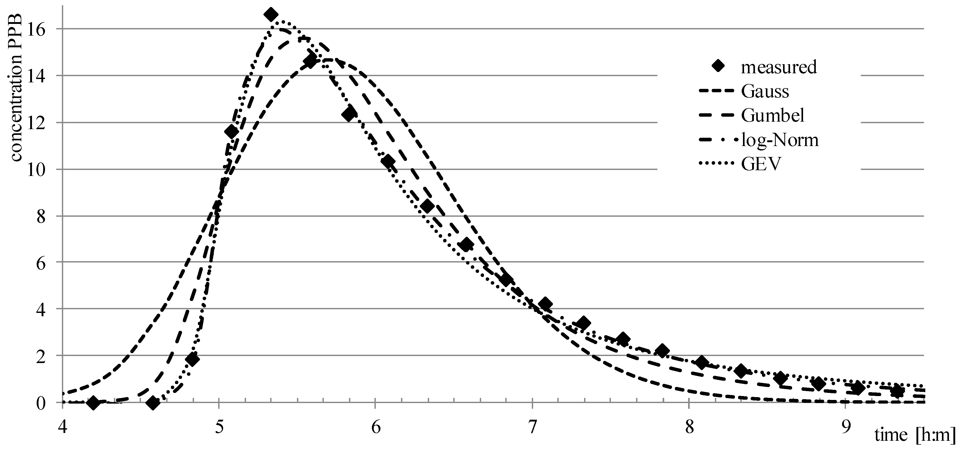
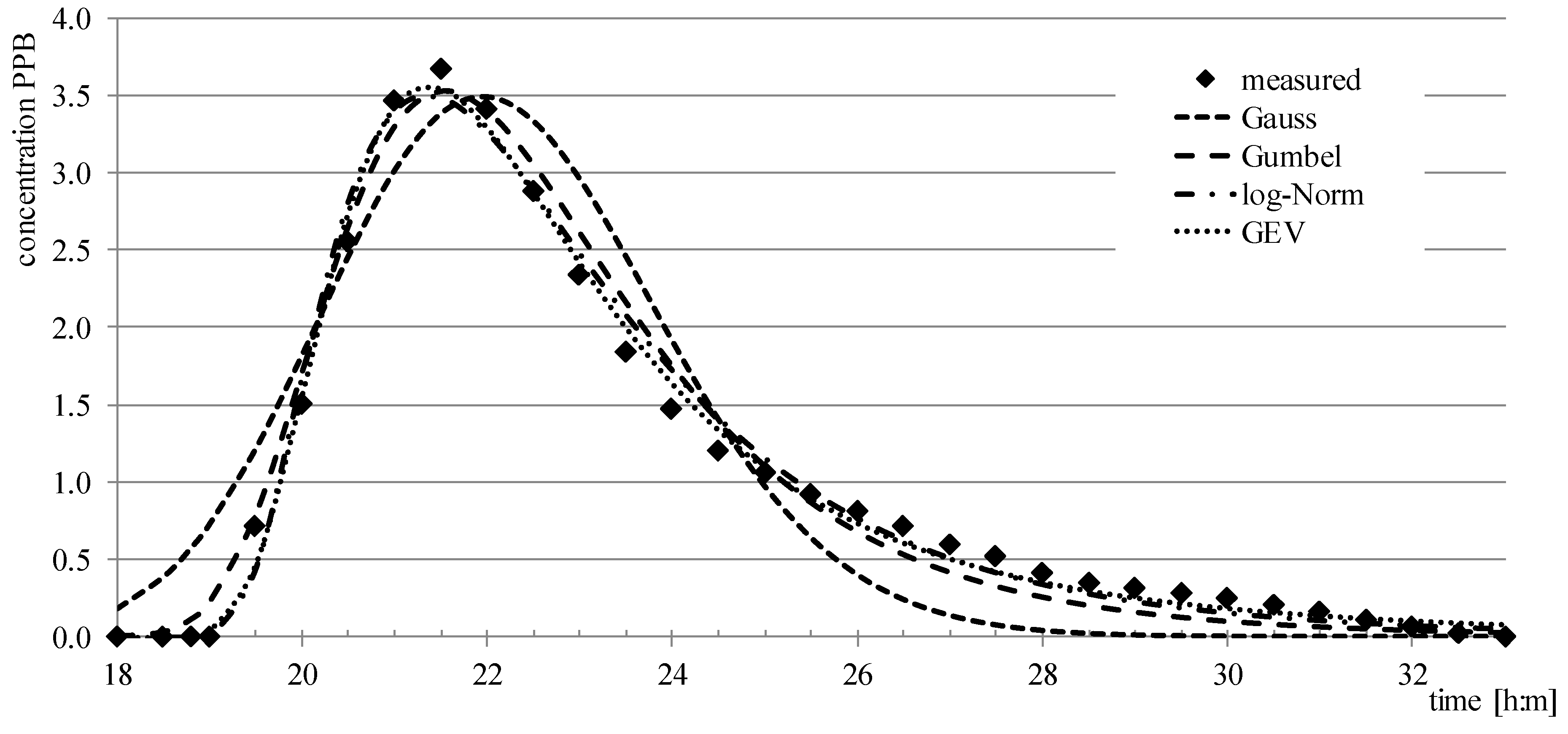
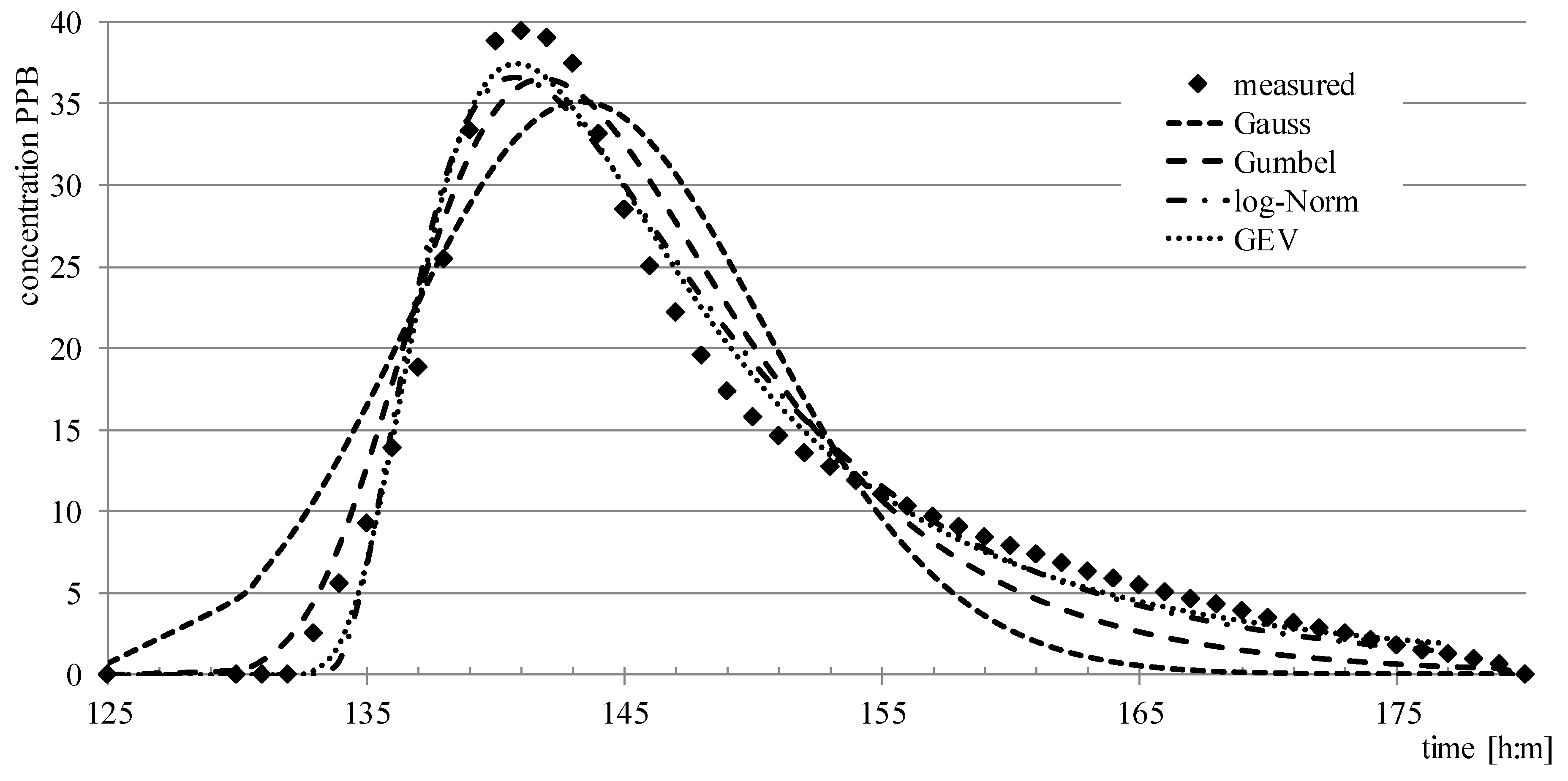
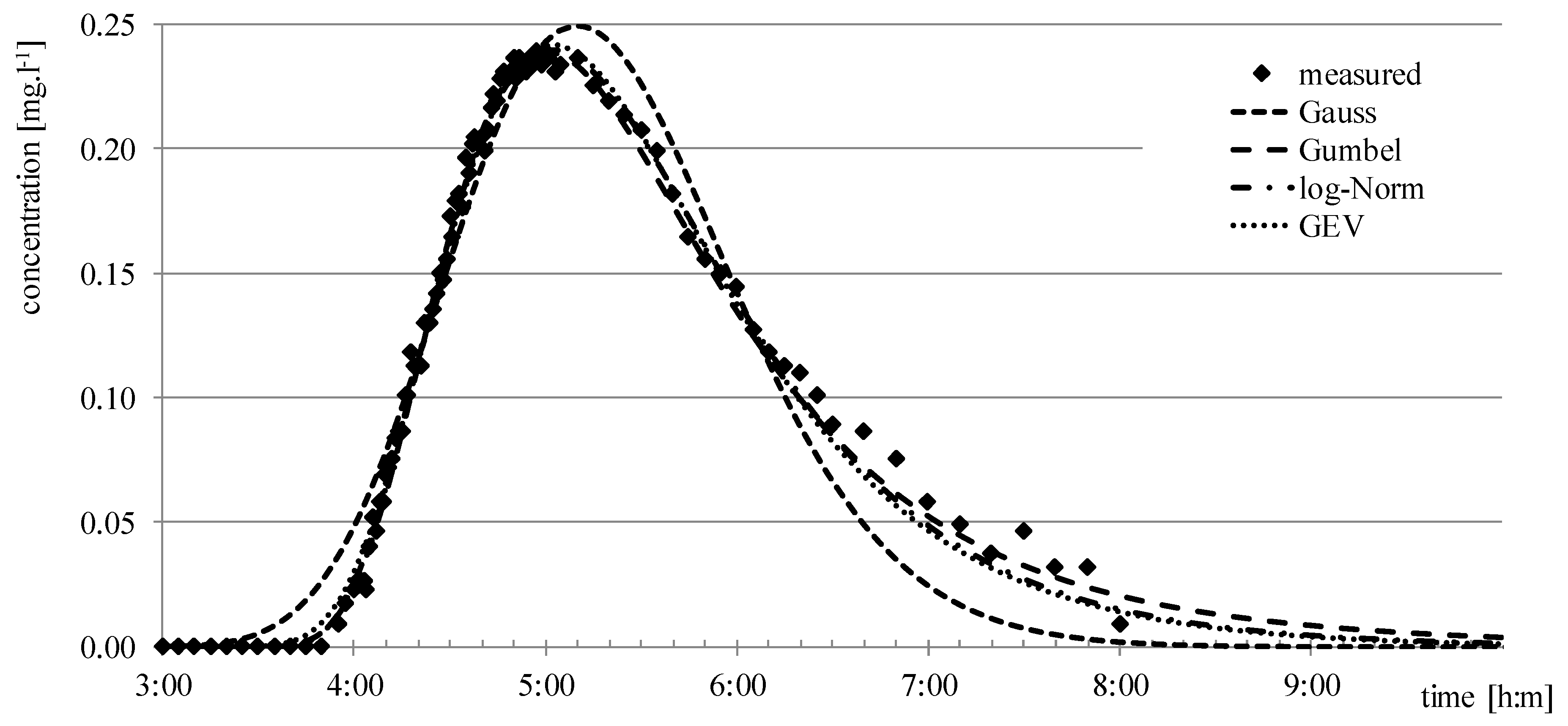
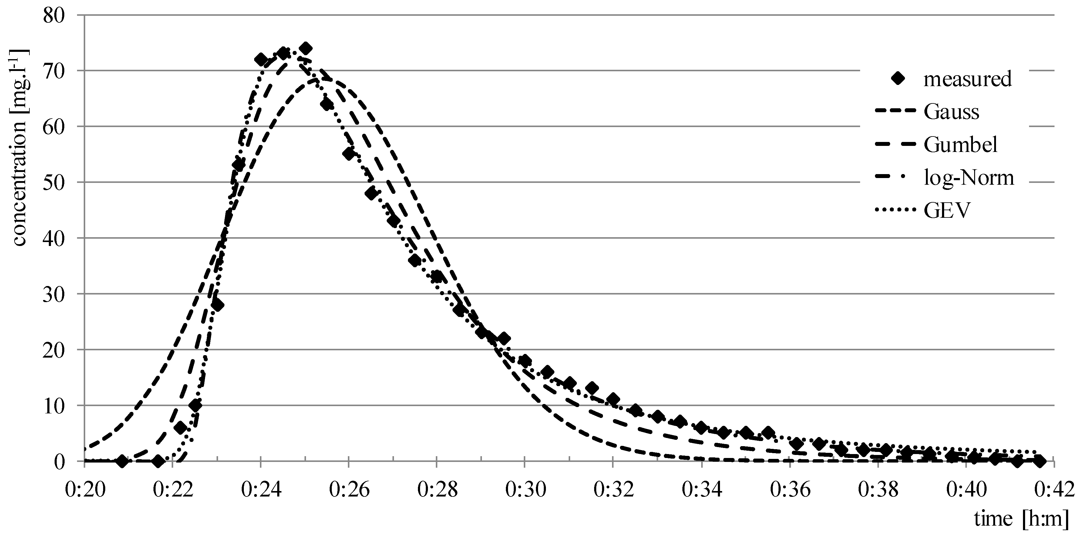
As a result, 29 tracer experiments with overall measurements in 141 profiles (there were up to 8 measuring profiles in each tracer experiment) were selected. Statistical evaluation was performed for each profile using each of the applied approximation methods (GaussD, GumbelD, LogNormD, and GEVD). This focused on finding the best fit between the measured values and the approximation with the considered method, i.e., to find the optimal set of method parameters providing the best goodness of fit based on the minimal root mean square error (RMSE) between the measured and approximated values, i.e.,
where RMSE is the root mean square error (kg.m
−3), c
m,t is the measured value (concentration) at the time
t (kg.m
−3), c
a,t is the approximated value in the time
t (kg.m
−3),
t1 is the measurement start time (sec) and
t2 is the measurement end time (sec), NRMSE (Eq. 24) is the normalized root mean square error (–), and
cmax and
cmin are the maximal and minimal concentration in each particular experiment (kg.m
−3).
The optimal set of parameters were analyzed and set up using the built–in Excel Solver function. The target value was the RMSE and the variable parameters were the peak time (mode), the scale parameter (to replace the term M/A in corresponding equations), and the corresponding method parameters (dispersion coefficient variance, shape parameters). The target value was the main indicator for the optimization process, looking for a minimum value for this indicator to achieve the maximum conformity of the measured and modelled data for the evaluated parameters. Limits for the peak time for the optimization process were typically set up from 0.8 up to 1.2 of the real (experimental) peak time to give some variability for the optimization process. Theoretically, there should be no limits, but by setting such limits, the convergence of the optimization procedure was secured. The scale parameter limits were set up to have a maximal difference of 0.001 (1‰) difference between the sum of the tracer in modelled and experimental values. There were just formal limits for other parameters, e.g., the dispersion coefficient should a nonzero and positive value, the lower boundary coefficient k (see (17) should be positive and less than 1 (0 < k < 1).
The considered rivers exhibited a large variability of hydraulic conditions. The length of the experiments was in the range from 2.5 up to 294 km (1.6–183 miles), while the range of discharges and velocity was from 0.48 up to 6824 m
3.s
−1 (17–241000 cfs—cubic feet per second) and from 0.07 up to 1.86 m.s
−-1, respectively. All the data are listed in
Table 1.
3.2. Field Experiments Data Use
The ability of the methods to approximate the 1D dispersion in extreme conditions of the channel with submerged vegetation in a large portion of the cross-sectional area was also tested.
For these tests, experimental data from three tracer studies in Malá Nitra, Šúrsky, and Malina streams conducted between 2012 and 2016 were used. These tracer experiments focused on the determination of longitudinal and transversal dispersion coefficients and on pollutant spreading within the primary mixing zone (prior to the transversal and vertical homogenization). In the first two streams, kitchen salt was used as tracer and the water conductivity was measured. For the experiment on the Malina stream we used a coloring agent (E133, brilliant blue) as a tracer, with subsequent spectrophotometric detection of agent concentration. In all the cases evaluated in this paper, an instantaneous input of the tracer was applied.
The discharge in all experiments was determined using the cross-section velocity method. For velocity determination the device SonTeK Flow 3D tracker was used. Water level slopes were determined using the GPS precise levelling method (with ±10 mm accuracy), and based on the water level slope, the roughness (Manning) coefficient was calculated using the Manning’s formula [
35].
The Malá Nitra stream is located within the village of Veľký Kýr (N48.181799°, E18.155373). The experiments were performed in two reaches with lengths of 785 and 1340 meters. The first reach of the stream was straight and the second was slightly curved in both directions (left and right bend). The channel at the bed was about 4 m wide with a bank height of 2.5 m and a bank slope of approximately 1:2. The discharge in selected experiments used for the method tests ranged from 0.230 up to 0.235 m3.s−1. The hydraulic roughness was n = 0.035 (Manning coefficient) and the water level slope was found to be approximately 1.5‰. The stream in the considered reach is prismatic with a width of 5.5 m and a water depth in the range from 0.4 to 0.6 m. The range of the determined longitudinal dispersion coefficient was from 0.5 to 2.5 m2.s−1. The experiments were performed in high summer (July 2012), when submerged vegetation was present to a large extent.
The second tracer study was carried out on a straight reach of the Šúrsky stream, located close to the village of Svätý Jur (Slovakia, N48.232957°, E17.202934°). The field measurements were made in a 300 m to 500 m long straight reach with a relatively prismatic cross-section profile. The discharge, the channel width, the maximum depth, and the average velocity were in the range 0.38 to 0.43 m3.s−1, 4 to 5.5 m, 0.4 to 0.8 m, and 0.245 to 0.282 m.s−1, respectively. The range of the determined longitudinal dispersion coefficient was from 0.63 to 0.98 m2.s−1. Field experiments were performed in spring (March 2014) when the presence of submerged vegetation was very low.
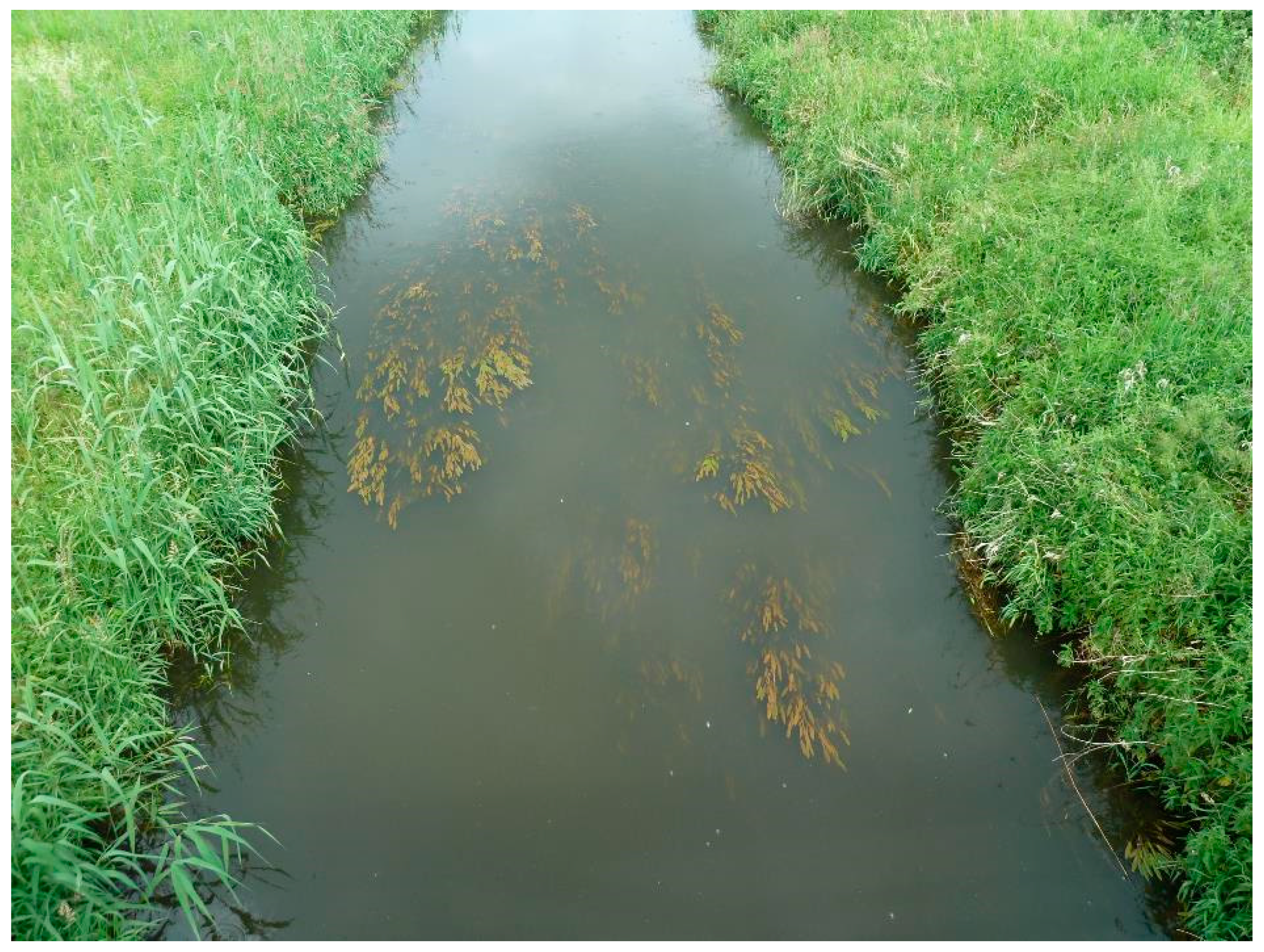
The last field tracer experiment was performed at the Malina stream in West Slovakia in 2016. Originally, the constructed cross-section profile was significantly influenced by vegetation. The measured discharge during the experiments was 0.408 m
3s
−1. The water level slope, specified by levelling measurements, was about 0.45‰. The stream shape in the examined stream section can be considered prismatic, the width was around 5 m, the average depth was 0.88 m with a maximum value of about 1 m. The dispersion coefficient was 0.95 m
2.s
−1. The experiment was performed in high summer (August 2016), with up to approximately one meter of emerged vegetation on the banks, as well as submerged vegetation in the central part of the channel. This vegetation on the stream banks and bed created dead zones for the flow. A picture of the vegetation and hydraulic conditions in this stream is shown on
Figure 4.
The main characteristics of all three streams used for tracer experiments in Slovakia are listed in
Table 2.
In all the three rivers used for field experiment data, the length was smaller than the length of rivers from the literature data. Therefore, the question of the 1D well-mixed assumption should be questioned.
Vertical mixing in a river needs, typically, a length of L
mix-vert = 100*h [
20], where h is the water depth. In the three Slovakian rivers, water depth h was always < 1 m (on average, 0.5, 0.6, and 0.88 m). So, L
mix-vert < 100 (from 50 to 88 m). This means in the field measurement the assumption of vertical mixing holds.
The estimation of the length for transversal mixing L
mix-transv is more difficult because no established theory exists to predict transverse mixing rate [
36]. This rate is related to several boundary conditions of the mixing process (riverbank/riverbed irregularities, vegetation, meandering, bends, islands, confluences). The vegetation is expected to affect Manning coefficient [
37], which is related to the friction factor, the shear velocity, and, ultimately, to the transverse mixing rate.
For scaling analysis, again, the length for transverse mixing is L
mix-transv = c
1*(W²/*h), where W is channel width and c
1 is a numerical constant related to the rate of the process of transversal mixing [
38]. In the three Slovakian rivers, c
1 could be in the order of 20–40, so the L
mix-transv should be in the order of 150–200 m, which is quite a lot shorter than the minimum distance of the field experiments (
Table 2). Hence, the assumption of complete mixing in the cross-section should be valid.


