Article

Site-Scale Integrated Decision Support Tool (i-DSTss) for Stormwater Management

1
Civil and Environmental Engineering Department, South Dakota School of Mines and Technology, Rapid City, SD 57701, USA
2
Civil and Environmental Engineering Department, Colorado School of Mines, Golden, CO 80401, USA
*
Authors to whom correspondence should be addressed.
Water 2019, 11(10), 2022; https://doi.org/10.3390/w11102022
Submission received: 20 August 2019 / Revised: 23 September 2019 / Accepted: 24 September 2019 / Published: 28 September 2019
(This article belongs to the Section Hydrology)

Abstract

:
A site-scale integrated decision support tool (i-DSTss) is developed for selection and sizing of stormwater Best Management Practices (BMPs). The tool has several component modules—hydrology, BMP selection, BMP sizing, and life-cycle cost analysis (LCCA)—integrated into a single platform. The hydrology module predicts runoff from small catchment on event and continuous basis using the Green-Ampt and Curve Number methods. The module predicted runoff from a small residential area and a parking lot with R2 value of 0.77 and 0.74, respectively. The BMP selection module recommends a BMP type appropriate for a site based on economic, technical, social and environmental criteria using a multi-criteria optimization approach. The BMP sizing module includes sizing options for green roofs, infiltration-based BMPs, and storage-based BMPs. A mass balance approach is implemented for all types of BMPs. The tool predicted outflow rates from a permeable pavement with R2 value of 0.89. A cost module is included where capital, operation and maintenance, and rehabilitation costs are estimated based on BMP size obtained from the sizing module. The i-DSTss is built on an accessible platform (Microsoft Excel VBA) and can be operated with a basic skillset. The i-DSTss is intended for designers, regulators, and municipalities for quick analysis of scenarios involving interaction among several factors.

1. Introduction

Urbanization impacts the quality of urban water resources, and ineffective stormwater treatment plays a major role. Land use change due to urbanization alters hydrological characteristics of watersheds by increasing impervious cover [1,2]. Consequently, stormwater infiltration is reduced and runoff is increased [3,4]. The United Nations Population Fund predicted that by 2030 more than 60% of the world’s population will live in urban areas [5]. Increased buildings, roadways, and parking lot densities associated with urbanization result in an expansion of impervious cover in urban watersheds. Thus, BMPs are implemented to achieve an integrated stormwater management [6]. The term BMP encompasses both structural (engineered or built infrastructure) and non-structural practices (operational or procedural practices; e.g., minimizing use of chemical fertilizers and pesticides) [7]. Green infrastructure (GI) is an evolving stormwater management approach using natural processes. Low impact development practices (LIDs) specifically emphasize better management of urban stormwater through reductions in post-development runoff by increasing on-site infiltration and reducing impervious surface cover [8].
GI solutions can be applied on different scales ranging from individual houses or buildings to a broader landscape level. At the largest scale, the preservation and restoration of natural landscapes (e.g., forests) are critical components of green infrastructure. On the local level, GI practices include rain gardens, permeable pavements, green roofs, infiltration planters, trees and tree boxes, and rainwater harvesting systems. Thus, at the local scale, the term GI may overlap with LID practices [9]. Across the nation, there is increasing interest in the use of LID practices as a means of reducing urban runoff and associated pollutant loads to receiving waters [1,10,11], and LID practices have become a common alternative to conventional stormwater solutions (e.g., grey infrastructures involving curb, gutter, sewer and storage systems) in urban watershed management. LID practices represent practices that are mainly implemented on-site to control stormwater at the source and restore natural hydrologic processes to pre-development conditions. In contrast, BMP is a broader term that includes both structural approaches and non-structural practices intended to reduce runoff and/or pollution from stormwater discharge [12]. The U.S. Environmental Protection Agency (EPA) considers LID practices as a stormwater control best management practice (BMP) and, along with other federal agencies, is encouraging the implementation of LID practices.
LID site design is typically based on factors such as area, depth, vegetation, and other site conditions including weather, precipitation amount, soil type, land use, slope, and percent impervious area [13,14]. LID practices are typically applied to mitigate hydrologic imbalances; however, inadequate attention has been given to the potential impacts on aquatic ecosystems and human health associated with stormwater contaminants. Although contaminant removal is not typically an explicit design criterion, infiltration-based LID practices usually improve water quality [15,16], yet BMP design for water quality improvement in engineered infiltration systems is often based on assumed performance or non-site-specific empirical estimation rather than premised on a fundamental understanding of pollutant removal mechanisms for the specific BMP at a specific site [17]. Thus, BMP design tools capable of more detailed analysis of peak flow reduction and water quality improvement are needed. More research is needed to properly characterize the interactions between hydrologic impacts of LID practices, processes for contaminant removal, and water quality performance. The BMP sizing tool within the i-DSTss includes a physically based mass balance approach for the design of infiltration and storage based BMPs.
Planning level decisions such as BMP placement are typically performed at the watershed scale [2]. Several watershed scale planning level tools have been developed for stormwater management (e.g., System for Urban Stormwater Treatment and Analysis IntegratioN (SUSTAIN)), however, these tools do not include detailed analysis for BMP sizing at the site-scale. These models are relatively complex, require extensive data processing, and modeling expertise to setup and operate. Other simplified tools are available that are based on empirical approaches. The prediction accuracy of these simplified tools is low relative to the more complex tools, and they are usually applicable to specific location where they were initially developed. The i-DSTss is a user-friendly tool that includes rigorous approaches used in the more complex tools (e.g., Storm Water Management Model (SWMM)). The tool includes an optimization approach for selection and sizing of BMPs at the site-scale. The BMP sizing module within i-DSTss can be used to design multiple types of BMPs based on user-defined flow reduction. The BMP selection module leverages resources from existing international stormwater BMP database and is designed to allow inclusion of new BMPs as they become available.

2. Overview of Decision Support Tools in Stormwater Management

The objective of this work is to develop an integrated site-scale Decision Support Tool that allows for selection and optimization of individual stormwater BMPs adaptable across the diverse climates and regional policies and practices. Stormwater management tools vary with respect to their capabilities and degree of complexity. Some have multiple component modules with ability to run hydrologic, water quality, and cost benefit analysis while others can handle only some of these processes. Some are developed for specific locations while others are applicable nationwide. Examples of such tools include the California Phase II LID Sizing Tool and the Minimal Impact Design Standards (MIDS) calculator that were developed for California and Minnesota states respectively. In contrast, other models such as SWMM and SUSTAIN can be applied in multiple locations nationwide. Some of the stormwater modeling tools include optimization feature with capability to iteratively determine the best solution (e.g., type and size of BMP). There are several other models without an optimization feature that are implemented in a simple forward-modeling (i.e., non-iterative) approach to evaluate alternatives where users can test ‘what if’ scenarios. This approach is time consuming and the solutions may not be optimal. Among the tools listed in Table 1, only EPA SUSTAIN and RSWMM-Cost include cost-based optimization approach for selection and placement of BMPs. Models with and without optimization features have been applied for design and assessment of performance of stormwater management systems and to compare alternative designs and operating policies. Optimization methods provide optimal values of system design and lead to the highest levels of system performance and can be used to eliminate inferior alternatives. The i-DSTss translates complex processes into an easy to use application with a graphical user interface for data inputting and displaying outputs. This feature allows the use of the tool by a broad range of users with different skillsets. However, the i-DSTss is not meant to replace other commonly used relatively robust stormwater tools such as SWMM with respect to hydrology and water quality analysis. A summary of existing stormwater management tools and their capabilities in comparison to i-DSTss developed in this study is shown in Table 1.

3. Methodology

The approach for the development of the comprehensive site-scale integrated decision-support tool, i-DSTss, involves creating individual modules and integrating the modules into a single modeling framework applicable nationwide. Specific steps in the development of the tool and relevant modules include:
(1) Development of a hydrology module: The hydrology module uses a physically-based approach and involves modification of existing approaches to develop a user-friendly computationally less-intensive module. This includes (a) translating implicit Green-Ampt and coupled manning’s and continuity equations into explicit equations, (b) developing approaches for tracking soil moisture and evapotranspiration for continuous simulation, and (c) translating Hargreaves equation from daily to sub-hourly for evapotranspiration calculation;
(2) Development of BMP selection module: This includes development of an automated optimization module to select cost effective BMP for a site considering stormwater quality, target water quality, removal efficiency of BMPs and other technical and economic criteria;
(3) Development of BMP sizing module: A physically based mass balance approach is implemented to estimate effective size of a BMP to meet runoff reduction for several types of BMPs including green roof system, infiltration and storage based BMPs;
(4) Development of LCCA module: A cost module is implemented to calculate the cost of BMPs based on the size determined using the BMP sizing module.
Procedures included in the development of each of these modules are provided below. Detailed procedures are provided under Appendix A. Appendix B includes a demonstration of the operation of the tool. To evaluate performance, the modules are compared to observations in Section 4.

3.1. Hydrology Module

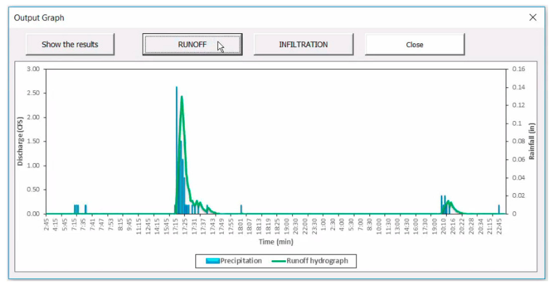
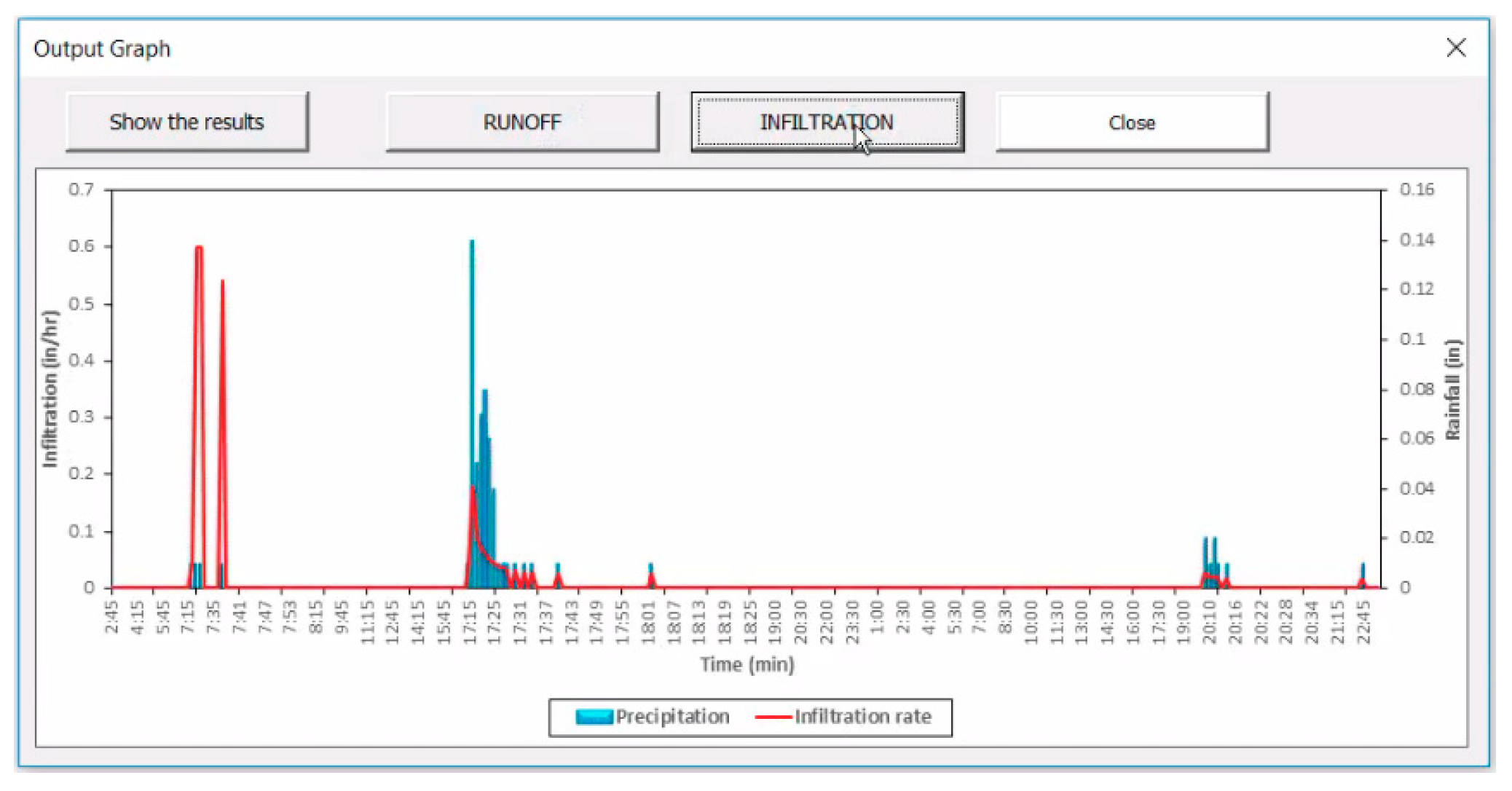
The hydrology module includes a graphical interface for data inputting and displaying outputs. Data inputs include rainfall, temperature time series, and soil data. The outputs include runoff depth and time series of infiltration rates and runoff hydrograph. The graphical user interface includes option for selecting methods for calculating infiltration losses (a Green-Ampt or modified Curve Number methods). The runoff depth estimated from precipitation and infiltration loss is transformed into a runoff hydrograph. The conceptual framework for the hydrology module is shown in Figure 1.
Rainfall-runoff simulation in i-DSTss includes both event and continuous based approaches. Event-based hydrologic modeling reveals how a site responds to an individual rainfall event. In contrast, continuous hydrologic modeling synthesizes hydrologic processes and phenomena over a longer time period that includes soil moisture tracking and its effect on infiltration and runoff. Several rainfall-runoff methods have been developed ranging from empirical approaches (e.g., Curve Number method) to physically based approaches (e.g., Green-Ampt model). Appropriate methods have to be selected based on the type of problem. In the subsequent sections, we present (1) the selection of rainfall-runoff methods, (2) event and continuous simulation approaches in i-DSTss, and (3) detailed procedures for the development and implementation of the various simulation options and rainfall-runoff methods in i-DSTss.

3.1.1. Selection of the Rainfall-Runoff Model

The selection of the rainfall-runoff model is often a compromise between model complexity (simple vs. complex) and availability of input data needed to setup and run the model [30]. The merits of simple versus more complex and physically based hydrologic models have been debated in literature [31]. Green-Ampt and Curve Number methods have been implemented in i-DSTss for runoff estimation. Green-Ampt is a simplified model of the infiltration process that contains realistic physics based on Darcy’s and the continuity equations and, at the same time, enables one to obtain an analytical solution [32]. The model assumes the soil above the wetting front is completely saturated and there is a sharp break in moisture content at the wetting front as water infiltrates into the soil. The Green-Ampt model has been the object of considerable development in the field of soil physics and hydrology due to its simplicity, physical basis, and satisfactory versatility for a wide variety of infiltration problems. Thus, it has been implemented in many of widely applied stormwater models. Another approach for estimation of rainfall excess is the Curve Number method developed by Soil Conservation Service (SCS), now known as the Natural Resource Conservation Service (NRCS) [33]. The Curve Number method is widely used because it is based on readily available input data such as land cover and soils data [20]. Both methods can be used for evaluation of peak runoff estimates for pre- and post-development conditions for the purpose of BMP sizing. The i-DSTss includes event-based and continuous simulation approaches presented in Section 3.1.2. Both Green-Ampt and Curve Number methods are used for event and continuous simulation of runoff within i-DSTss.

3.1.2. Event-Based and Continuous Simulation

An event-based model represents a response to an individual isolated rainfall event over a relatively short period of time ranging from about an hour to several days (e.g., volume of surface runoff, peak runoff, and time to peak). A continuous hydrologic model represents hydrologic responses to a number of rain events and their cumulative effects over a longer duration that includes both wet and dry periods. When long term analysis involving life cycle cost is needed, the continuous simulation option within i-DSTss can be used. Continuous simulation is data intensive and requires tracking soil moisture and evapotranspiration. In contrast, event-based simulation is less data intensive and does not require tracking soil moisture content or evapotranspiration. Event based simulation is frequently used in the design of hydraulic structures, however, when there is a need for long term impact assessment, continuous simulation becomes important.
(a) Event-based runoff estimation module: The site-scale tool has an event-based model for estimation of runoff for design storm events. At times, this may be the only level of tool that is required by planners to provide flood estimates, or it may be applied when data is not sufficient to justify a continuous simulation model.
(b) Continuous simulation runoff module: The continuous simulation model is operated over a longer period of time, which includes time series of rainfall events and inter-storm conditions. The model accounts for changes in soil moisture and its impact on infiltration. The soil moisture accounting includes an option where soil moisture content is set back to dry condition if water input or rainfall ceases for specified period of time depending on the soil type. The approach used to track soil moisture content for continuous simulation in i-DSTss is based on the method implemented in SWMM model [20].
Both event-based and continuous simulation methods in i-DSTss are built on an Excel-VBA platform to facilitate integration to other modules within the i-DSTss that are developed on the same platform (BMP selection, sizing, and cost modules). Detailed procedures are presented in Section 3.1.3 and Appendix A.

3.1.3. Estimation of Runoff Depth and Hydrograph

The runoff estimation approach is based on conservation of mass (the continuity equation). The change in runoff depth (dD/dt) or volume (dv/dt) is calculated using a mass balance approach considering precipitation intensity (i), evapotranspiration rate (e), infiltration rate (f), and runoff rate (Q) as described in Equations (1) and (2) below. Thus, the rate of change of volume and depth of flow is given by:
d v d t = A d D d t = A × ( i e f ) Q
Dividing by the area of the site and replacing the discharge rate, Q with modified Manning’s expression we get coupled continuity-Manning’s equation given by:
d D d t = i e f w × s 1 2 A × n ( D d p ) 5 3
where v is volume of runoff from the site ( m 3 ), A is area of site ( m 2 ), i is intensity of rainfall (m/s), e is evapotranspiration rate (m/s), f is infiltration rate (m/s) calculated using Green-Ampt or Curve Number method, Q is discharge rate (cubic meters per second (cms)), w is width of site (m), s is slope of site (m/m), n is manning’s roughness coefficient, t is time step (s), D is depth of runoff (m), and d p is depth of depression storage (m). Equation (2) is used to estimate the depth of runoff and flow based on i, f, and e. Methods of estimating evapotranspiration (e) and infiltration rates (f) in Equation (2) are presented below.
Evapotranspiration (e): Evapotranspiration in Equation (2) is estimated based on a modified temperature-based evapotranspiration equation developed by Hargreaves [34]. The method requires fewer input parameters and gives reasonable estimates of evapotranspiration. The initial version of Hargreaves equation for evapotranspiration is based on daily time steps. The equation was modified to disaggregate the daily evapotranspiration estimates into sub-hourly estimates using a cosine function given by:
E T s u b h o u r l y = E T d a i l y × ( 0.1302 × Δ t × cos ( 2 π × ( 11.23 + t ) 24 ) )
where Δ t is time step (h) and t is cumulative time (h). Equation (3) gives an estimate of diurnal distribution of daily evapotranspiration based on previous studies [35,36].
Infiltration rate (f): Initially, an implicit Green-Ampt infiltration formulation was evaluated. The implicit Green-Ampt formulation required a longer simulation time. To reduce the simulation time, an explicit method was applied in i-DSTss. After extensive review and comparison of several explicit approaches, an explicit Green-Ampt approach presented by Barry et al. [37] was selected. The explicit approach was compared to the implicit approach and the results were very similar for different soil types [38]. This explicit method uses the W-Lambert function to solve the natural logarithm equation in the Green-Ampt infiltration equation. In i-DSTss, the infiltration rate obtained using explicit Green-Ampt equation or Curve Number method can be used to calculate the depth of runoff using Equation (2). f and e estimated using the approaches discussed above are used to estimate runoff depth using coupled continuity-Manning’s equation (Equation (2)).
Equation (2) is also implicit and can only be solved iteratively. The implicit equation given by Equation (2) was also converted to an explicit equation following the approach by Mizumura where an exponential equation is approximated with a quadratic equation by adding curve fitting coefficients [39]. Equation (2) was modified using this approach to yield:
{ 0.730 × W C O N × Δ t 4 } x 2 + { 0.730 × W C O N × Δ t × ( D 1 d p ) 1 + 0.292 2 × W C O N × Δ t } x        + { 0.730 × W C O N × Δ t × ( D 1 d p ) 2 + 0.292 × W C O N × Δ t × ( D 1 d p )        + 0.0146 × W C O N × Δ t + i * × Δ t } = 0          
After solving this quadratic equation D 2 will be equal to x + D 1 .
Where W C O N = W S 1 / 2 A n , i * = i e f and x = D 2 D 1 where D2 and D1 are depth of runoff in time step 1 and 2. Equation (4) is computationally less intensive than Equation (2). Additional details describing calculation of runoff are provided in Appendix A.

3.2. BMP Selection Module-Optimization Approach

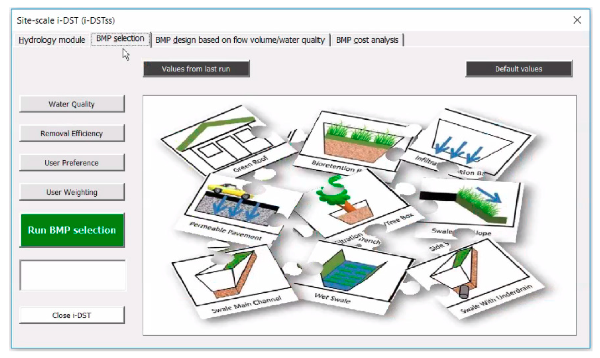
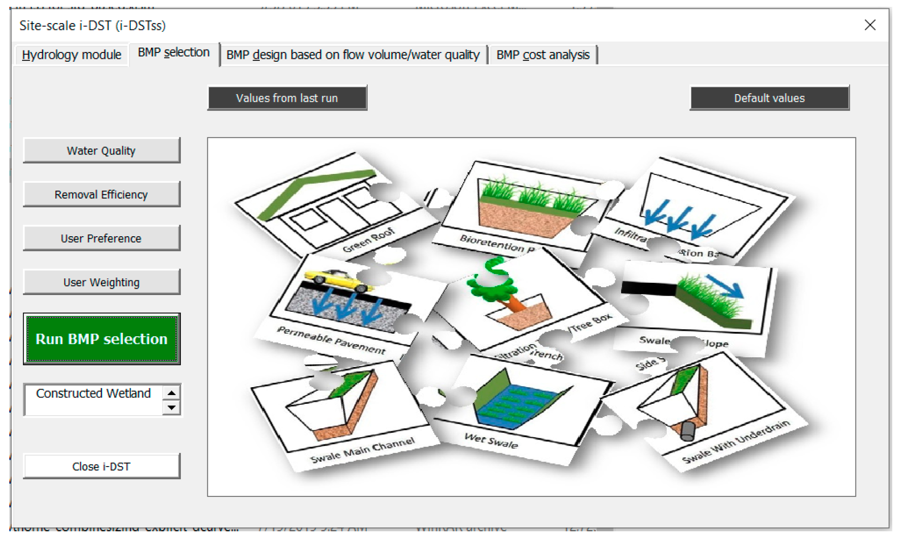
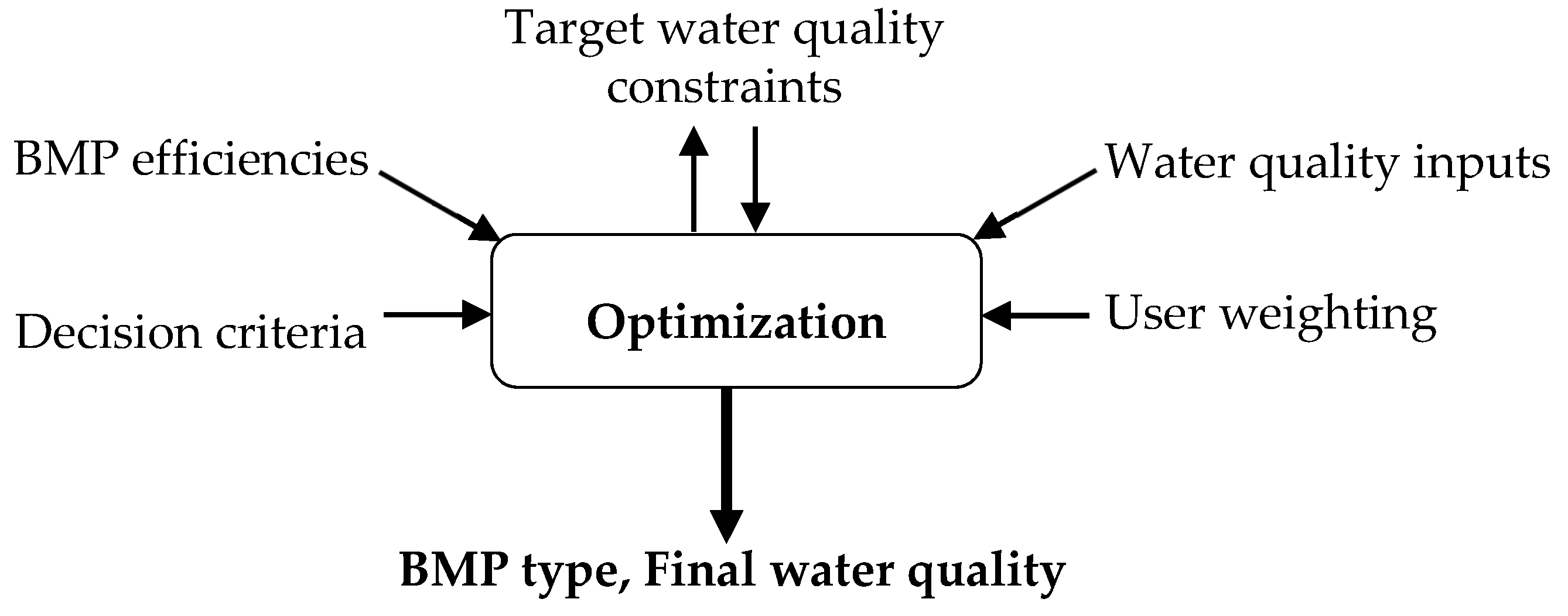
The conceptual framework of BMP selection module is shown in Figure 2. The BMP selection module includes several components integrated into an optimization module that uses an iterative process to generate optimal solutions (solutions that satisfy all of constraints with respect to the multiple objective functions). Inputs to BMP selection module include influent water quality data, list of BMPs and BMP efficiency, target water quality, decision criteria, and weights. Several BMPs are included in the BMP selection module including green roof, rain barrel, cistern, bioretention, grass swale, rain garden, sand filter, dry well, infiltration trench, infiltration basin, box tree, porous pavement, wetland, dry pond, and wet pond. Also, two types of BMPs, vegetated filter strip (VFS) and forebay, were added as a pre-treatment.
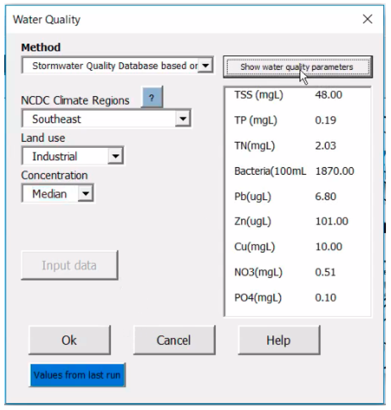
The optimization module evaluates the inputs and selects the best BMP type iteratively with respect to decision criteria including BMP cost while meeting target water quality requirements. The BMP selection module has a built-in water quality database assembled from the National Stormwater Quality Database (NSQD) [40]. This allows users to query the minimum, median or maximum concentration for each pollutant based on National Climatic Data Center (NCDC) climate region, land use and level of pollutant concentration to obtain influent water quality data. The land use categories in the national stormwater quality database include commercial, freeways, industrial, institutional, open space and residential sites. The tool has an option for users to input site specific water quality data if available. The tool also allows specifying target water quality requirements for each of the constituents. Based on input and target water quality, the level of treatment required is calculated for each pollutant. BMP efficiency for each BMP type is obtained from international stormwater BMP database [41]. The tool calculates the treatment efficiency required for each of the pollutants and selects a BMP type that meets the required treatment efficiency.
A linear optimization approach is implemented for BMP selection. The optimization process begins with defining an objective function and constraints. The objective function consists of multiple decision factors including environmental, economic, social and technical criteria. Meeting target water quality is a priority in the optimization process. There are other features included to provide additional flexibility to the tool such as ability to include or exclude BMPs from the selection process. When multiple criteria are involved in the decision-making process, a multi-objective optimization that includes more than one objective function is developed and all the objective functions are optimized simultaneously. The process usually involves optimizing the objective function with respect to some variables in the presence of constraints on those variables. In this study, the objective function is based on multiple decision criteria, thus, it is defined as a Multi-Objective Optimization. In the subsequent sections, we present (1) The Multi-Objective Optimization (MOO), (2) the objective function, and (3) the constraints.

3.2.1. Multi-Objective Optimization (MOO)

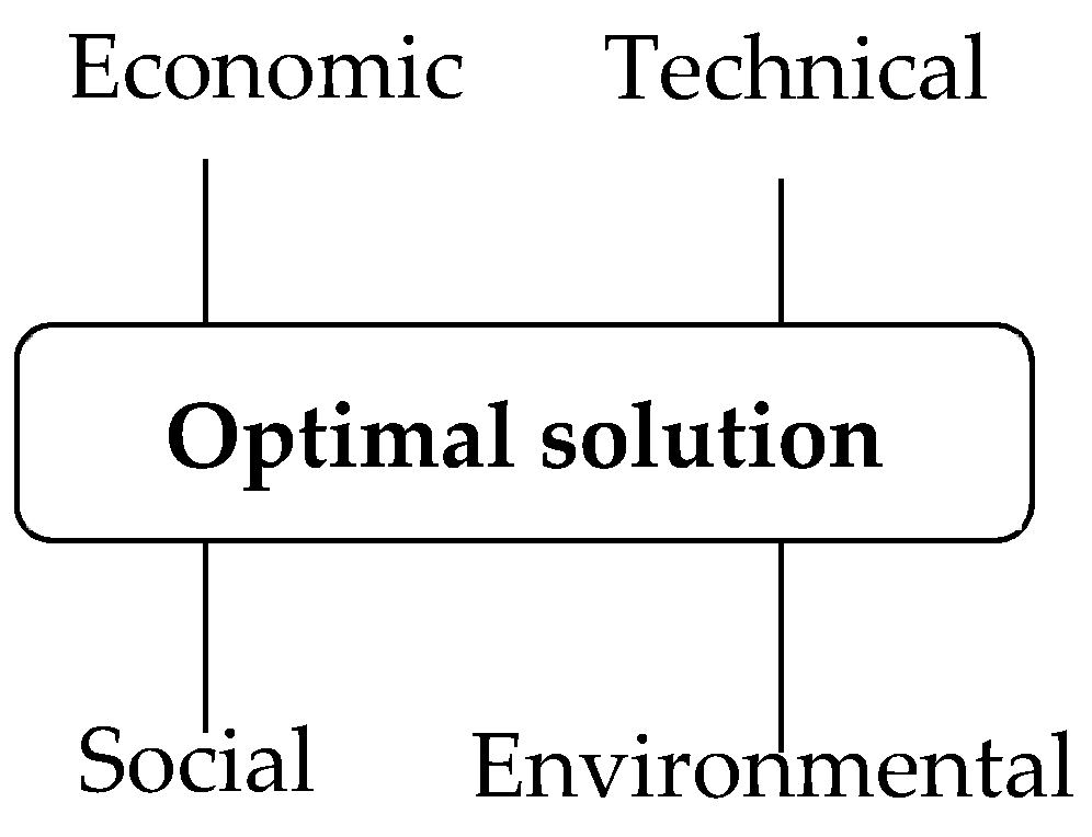
The i-DSTss selects a BMP based on multiple decision criteria (environmental, economic, social, and technical criteria) using MOO approach. MOO concept has already been applied in other researches in urban hydrology and treatment process selection [29,42]. MOO techniques may include multiple conflicting criteria (e.g., economic versus technical) and thus, involve a trade-off between multiple objectives. Analytic Hierarchy Process (AHP) involves assigning weights to different alternatives and a pair-wise comparison of alternatives is used to evaluate trade-offs [43]. In MOO method, multiple alternatives can be compared simultaneously and multiple objective functions are converted into a single objective function and solved as a single optimization problem. The solution in a single objective optimization can be regarded as optimal when the objective function achieves the smallest or largest value (for minimization or maximization problems, respectively) within the solution space defined by constraints. When dealing with conflicting objective functions, the solution can be seen as pareto optimal where no objective function value can be improved without compromising some other objective function value (Figure 3) [44]. When quantities included in the objective function are different (e.g., technical versus economic) normalization can be used to ensure consistency of the optimal solution. The normalized objective functions can be defined using a weighted sum approach. Weights are usually applied to each criterion or objective function based on professional judgment regarding the importance of each criterion to the decision-making. The MOO problem can be converted to a single-objective mathematical optimization problem using a weighted sum method. In a weighted sum method, the single objective function is constructed as a sum of objective functions multiplied by weighting coefficients.

3.2.2. The Objective Function

The i-DSTss selects a BMP type for a site based on environmental, technical, economic and social criteria (discussed earlier) while meeting target water quality or level of treatment defined as constraints in the optimization module. A list of criteria, sub-criteria, and a description is provided in Table 2. Each BMP is assigned weights and ranked based on these sub-criteria. The weights, defined by the user, reflect the importance of each sub-criterion in the BMP selection process. Ranks are defined by experts and are used to reflect the merit of each BMP with respect to a criterion. That is, weights consider only the relative importance of a criterion, while rankings compare the relative suitability of each BMP with respect to a criterion. The weights are assigned qualitatively ranging from 0 to 5, with a weight of 1 indicating a criterion is less important to the decision-making compared to another criterion with a weight greater than 1. Users can assign a weight of zero to one or more of the criteria to exclude the criteria. This may lead to the use of fewer and most relevant criteria (e.g., only economic criterion) in the decision-making. A total score reflecting both weights and ranks is calculated for each BMP which serves as a basis for comparison of BMPs in the BMP selection process. The total score, S, defined as the sum-product of rankings and weights:
S = i = 1 m w i R i
where wi is weight assigned by the user to criterion i, Ri is expert assigned ranking to a BMP based on criterion i. i varies from 1 to m where m is the number of criteria (listed in Table 2). S (calculated for each BMP) refers to the sum-product obtained by multiplying the weights and ranks and summing up the products. If two BMPs meet the target water quality, a BMP that has a lower combined score S is preferred to a BMP with relatively high total score. The objective function is defined as the sum of scores (ΣS) where S is a score for one BMP. Thus, the multi-objective optimization problem is defined as:
O b j   V a l = min j = 1 n S j X j
where Obj Val is the value of the objective function (total scores considering all BMPs), Sj is combined score calculated for one BMP using Equation (5). Xj is a binary decision variable with a value of 0 or 1 and n is number of BMPs. During the optimization process, Xj becomes zero if a BMP is not selected and 1 if selected. The goal is to minimize Obj Val (e.g., cost if cost is the only criterion). Thus, a BMP type is selected based on achieving minimum Obj Val. Note that this is subject to constraints that are chosen by the user, discussed below.

3.2.3. Constraints

The BMP selection module is formulated such that the best BMP is selected with respect to a set of criteria while meeting user defined constraints. Target water quality requirement for each pollutant is defined as one of the constraints that has to be met by the BMP selected. Meeting the target water quality requirements is a priority in the BMP selection process. There are other constraints that are included to provide further flexibility to the user. For instance, users/utilities may want to include or exclude a BMP because of some site-specific reasons. The inclusion of such constraints in the optimization model makes the i-DSTss a flexible tool compared to other tools discussed earlier.
Target water quality constraint: Each BMP has a specific removal efficiency for specific pollutant. The stormwater must be treated to meet the target water quality specified by the user or a standard defined based on regulation. Thus, the process requires defining removal efficiency of each BMP. Data on BMP removal efficiencies from International Stormwater BMP Database [41] is incorporated into the tool. Removal efficiency required to meet target water quality is calculated as:
R e m o v a l   e f f i c i e n c y   r e q u i r e d   ( % ) = ( I n p u t   w a t e r   q u a l i t y T a r g e t   w a t e r   q u a l i t y ) I n p u t   w a t e r   q u a l i t y × 100
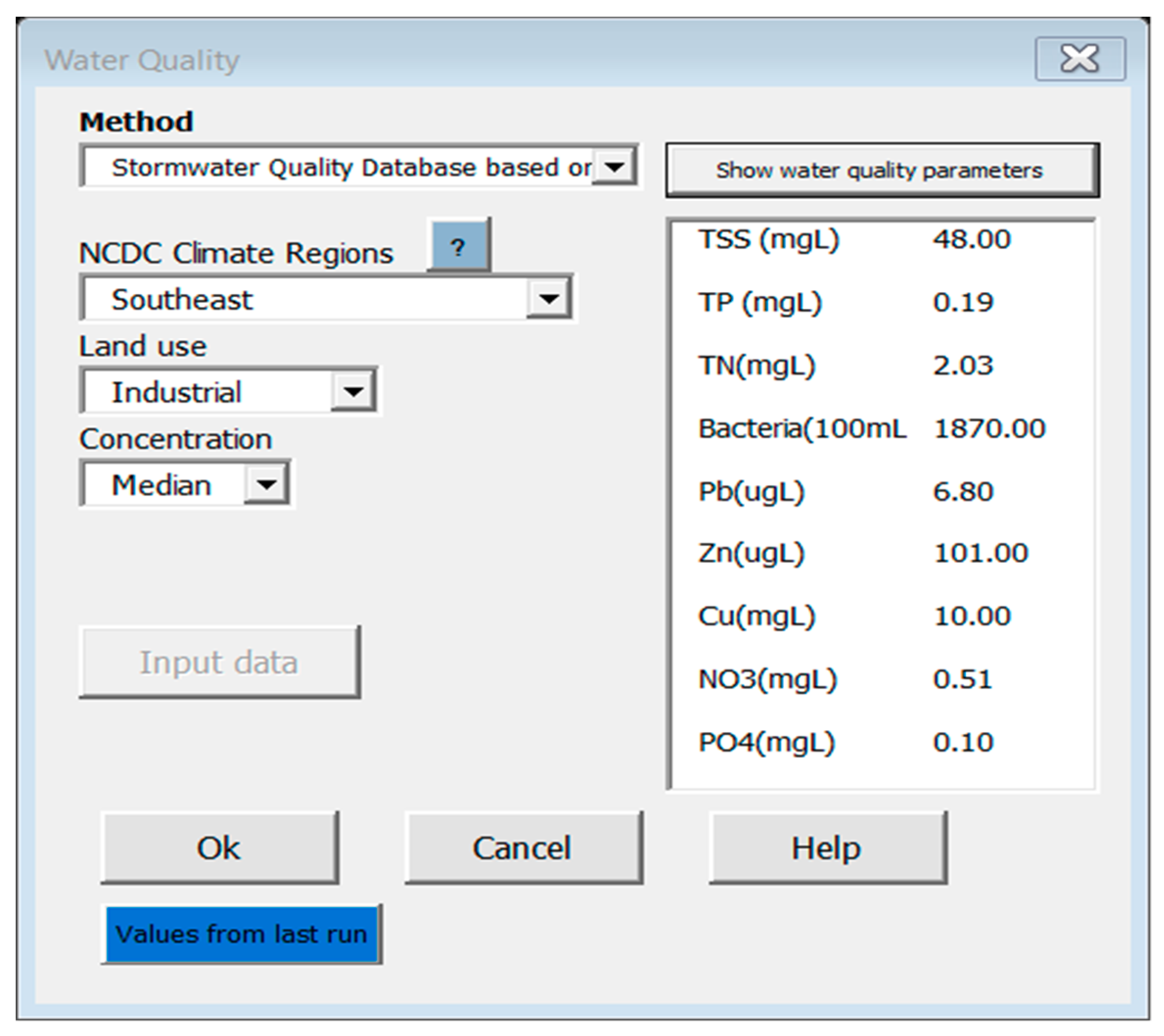
Input water quality in Equation (7) is obtained from NSQD [40]. The NSQD, originally developed based on EPA rain zone, was rearranged by NCDC climate regions and used as database for BMP selection module. Users can select Minimum, 1th quartile, median, 3th quartile or Maximum percentile concentration levels (Figure 4). When the user selects a region, land use and concentration levels, the input water quality data is automatically retrieved from the water quality database. Alternatively, the user can manually enter water quality data specific to the site or based on local event-mean concentrations (EMCs). Pollutants included in the water quality database include TSS, TN, TP, Zn, Cu, Pb, NO3, PO4 and Bacteria (Total Coliform). The target concentration can be set to water quality standard from EPA or user input values. The tool automatically selects a BMP type with treatment performance (removal efficiency) that exceeds the required removal efficiency calculated using Equation (7). The treatment performance is obtained from the International Stormwater BMP database.
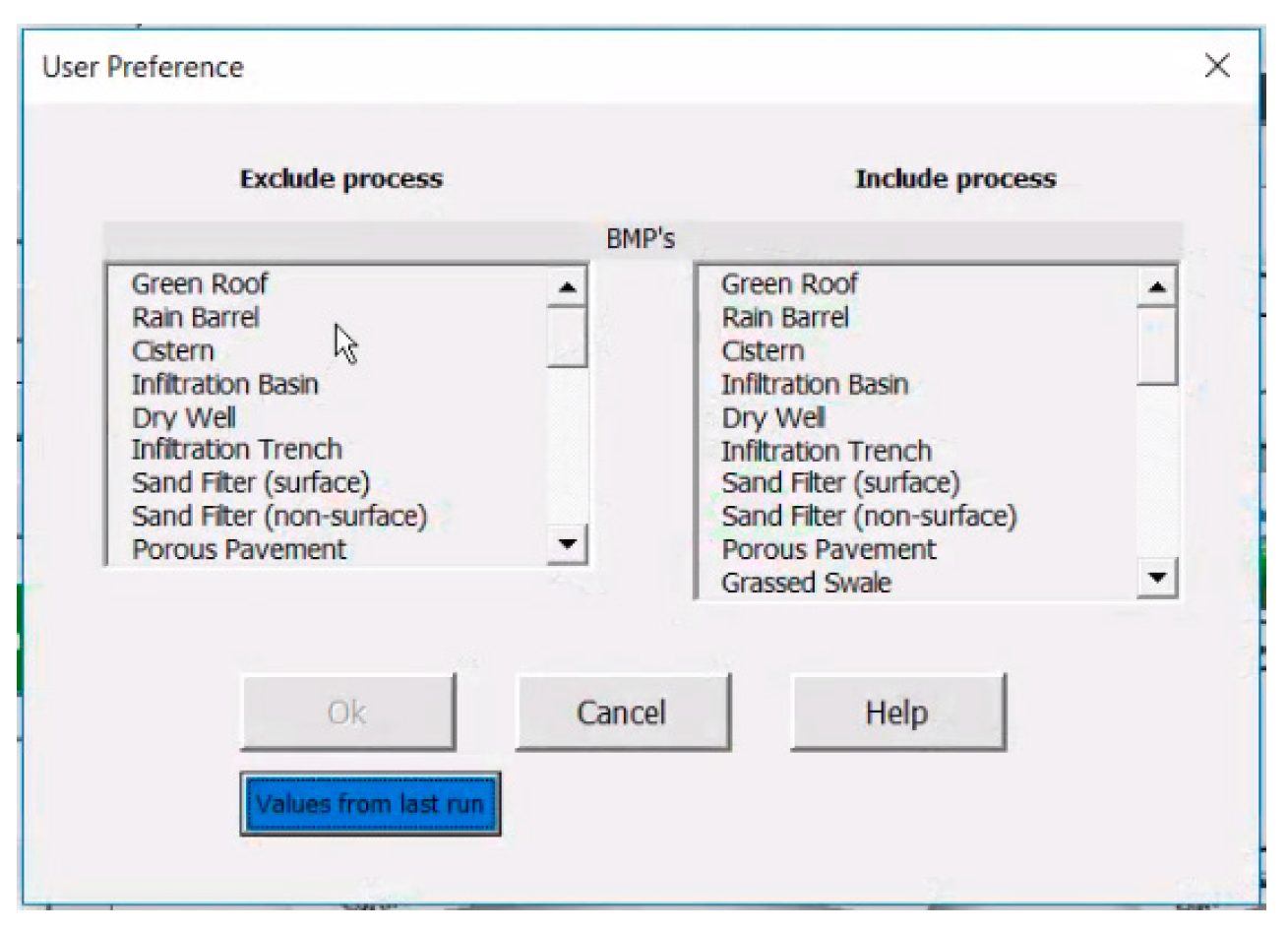
BMP inclusion option: The BMP selection module selects the best BMP option with respect to all criteria including cost that meets the target water quality requirement. However, users may want to keep an existing BMP or may want to include a BMP for site specific reason. The BMP inclusion option within the i-DSTss will include this BMP and add additional BMP if required to meet the target water quality.
BMP exclusion option: A user may want to exclude a BMP type from the selection process for some site-specific reason. The BMP selection module provides flexibility to exclude a BMP from the list.

3.3. BMP Sizing Module

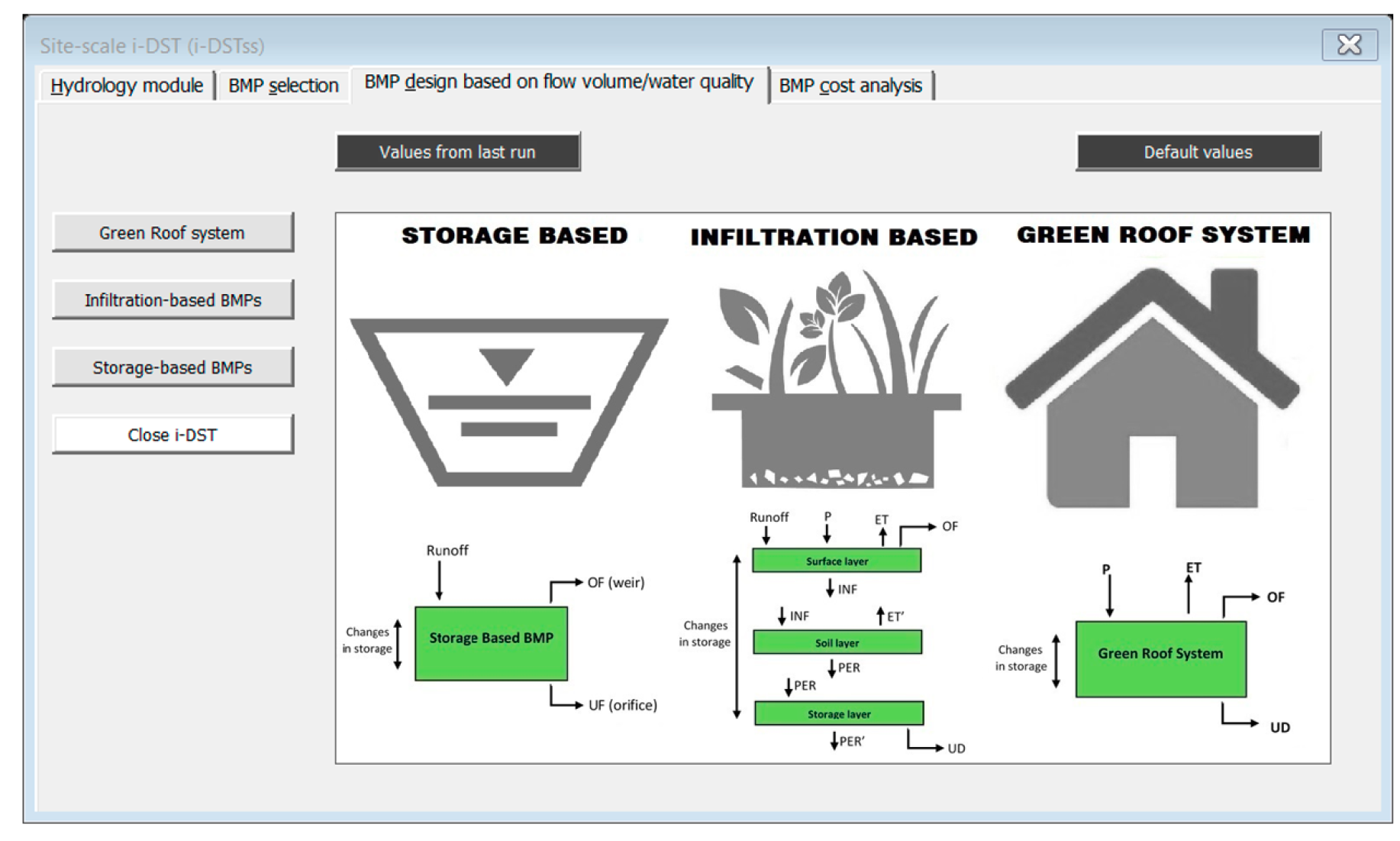
The BMP sizing module is developed to size BMPs based on user-defined percent flow reduction. The BMP could be designed to capture and treat the first flush (e.g., first half-inch of rainfall) or any other user specified percent flow reduction. The tool provides a more flexible option than other simplified approaches that are based on only capturing and treating the first flush. BMPs are classified into three different categories for the purpose of sizing, including: Green roof system, infiltration-based BMPs, and storage-based BMPs.
The BMP sizing tool allows design based on a single or continuous rainfall event. BMPs are traditionally designed based on a single-event rainfall (design storm approach) where peak runoff or volume reduction are used as criteria for BMP design and the designs are usually based on the bigger events. However, during preliminary testing, we observed that a relatively smaller storm event preceded by larger antecedent rainfall could be more critical for sizing than a bigger event with no antecedent rainfall condition. This demonstrates the advantage of tracking soil moisture and water level (storage) in infiltration-based and storage-based BMPs using a continuous simulation approach. The option allows users to evaluate an event or continuous simulation approach and select a more conservative design.
A mass balance approach was applied in the development of all types of BMPs. It is anticipated that the physically based mass balance approach will improve the accuracy of BMP sizing compared to the empirical approaches. For green roof system and infiltration-based BMPs, surface area of BMP is determined based on percent volume captured whereas for storage-based BMPs, a BMP volume, surface area, and outlet geometry are determined based on peak flow reduction. Additional details about the sizing procedures for each BMP category is discussed below and under Appendix A.

3.3.1. Green Roof System

The mass balance approach was applied for green roof system where water input to the green roof system is precipitation and the losses are evapotranspiration, overland flow and underdrain and the difference is change in storage. The water balance equation is given by Equation (8) below.
i E T U D O F = Δ θ Δ t d s o i l
where i is precipitation intensity (mm/h), ET is evapotranspiration rate (mm/h), UD is underdrain rate (mm/h), OF is overflow rate (mm/h), ∆t is time step (h), ∆θ is changing in soil moisture, and dsoil is depth of soil/media (mm). Multiplying the rates by the time step we get:
P E T ' U D ' O F ' = Δ θ × d s o i l
where P is precipitation (mm), ET’ is evapotranspiration (mm), UD’ is underdrain (mm), and OF’ is overflow (mm). Overflow refers to part of the inflow that does not infiltrate or become underdrain discharged through an overflow system. Underdrain refers to flow that originates from gravity water held between field capacity and saturation.
Possible conditions for ET’, UD’ and OF’ calculation included in the model are:
(a)
If   θ < θ W P no   transpiration   , E T ' = E T   calculated   using   Equation   ( 3 ) ,   O F ' = 0 ,   and   U D ' = 0
(b)
If   θ W P θ θ F C E T ' = M i n   ( E T   calculated   using   Equation   ( 3 ) ,   ( θ θ W P ) × d s o i l ) ,   O F ' = 0 ,   and   U D ' = 0  
(c)
If   θ F C < θ < θ s E T = M i n   ( E T   calculated   using   Equation   ( 3 )   and   ( θ F C θ W P ) × d s o i l ) ,   O F = 0   , and   U D ' = ( θ θ F C ) × d s o i l  
(d)
If   i > k s ,   θ = θ s   no   transpiration   , E T = E T   calculated   using   Equation   ( 3 ) O F = ( i k s ) × Δ t ,   and   U D ' = ( θ s θ F C ) × d s o i l
Where θ is calculated soil moisture content, θ W P is soil moisture content at wilting point, θ F C is soil moisture content at filed capacity point, θ s is soil moisture content at saturation, i is precipitation intensity, ks is saturate hydraulic conductivity, Δt is time step and dsoil is depth of soil.
For conditions (a) to (c), θ is calculated using Equation (9). For the last condition (d), the soil is assumed to be saturated, because for green roofs, saturation may occur in a relatively short period of time particularly for high intensity rainfall (i > ks). Based on this assumption, the overflow can be estimated as OF’ = (iks) × ∆t. Based on Feddes model the transpiration ceases when soil is saturated while evaporation may occur, which is calculated using Equation (3) [45].

3.3.2. Infiltration-Based BMPs

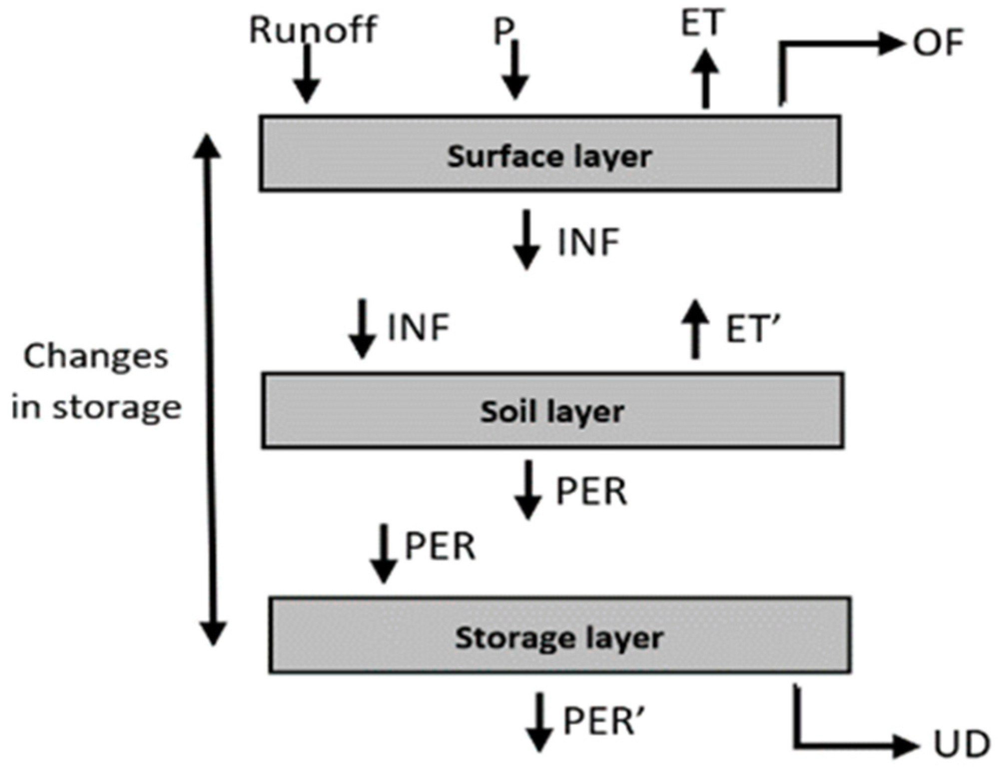
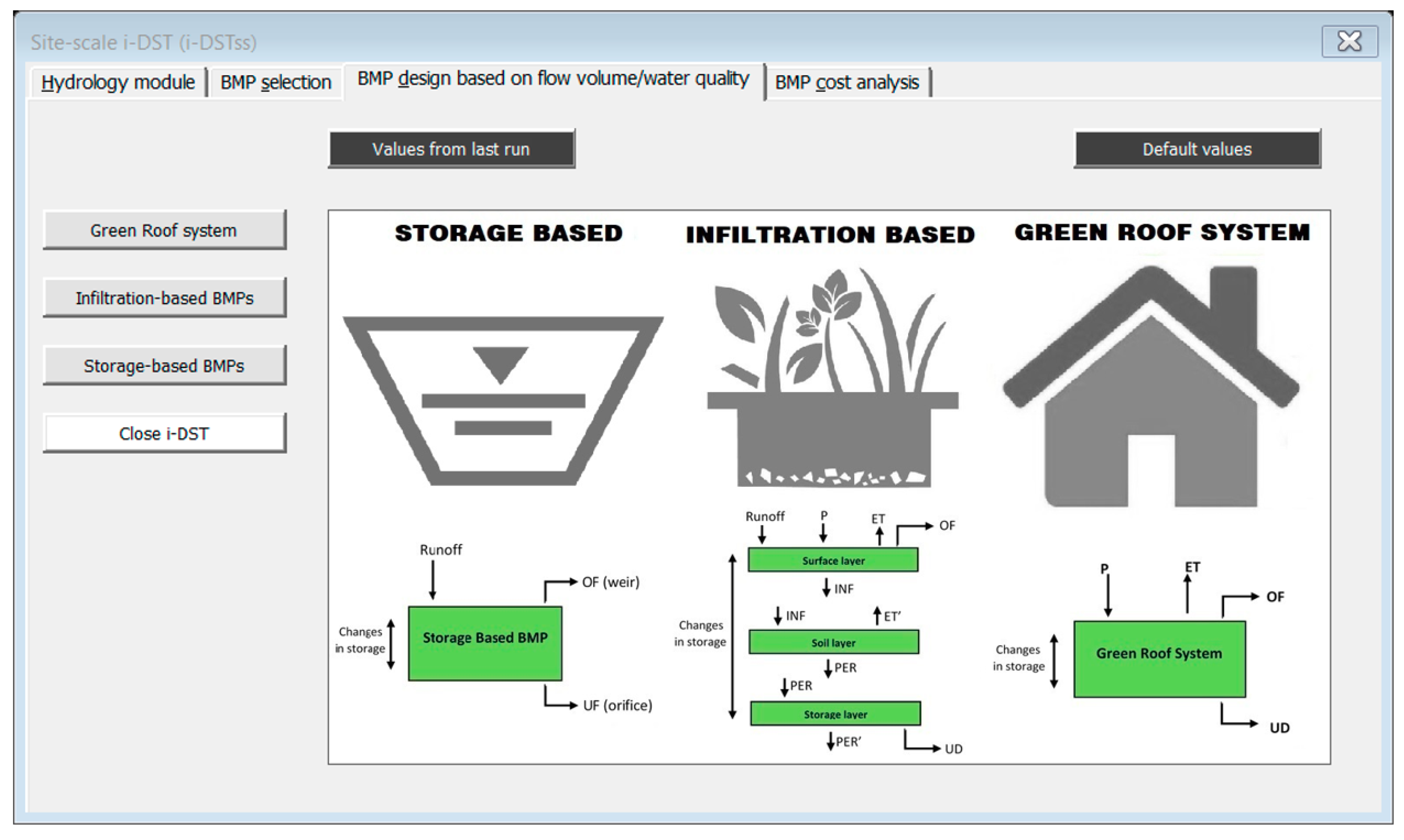
A mass-balance approach was implemented for infiltration-based BMPs for each layer where the outflow from the top layer becomes inflow to the next layer. The number of layers vary in infiltration-based BMPs with some BMP having three layers (surface/ponding layer, a soil layer and a storage/gravel layer) and others with only a surface layer or a combination of surface layer with either soil layer or storage layer (Figure 5). Thus, Infiltration-based BMPs are classified into four groups to account for the variations in the laying system:
(a)
Infiltration-based BMPs with both soil layer and storage layers: Porous pavement, Grass swale (with surface layer), Bioretention (with surface layer), Sand filter (non-surface);
(b)
Infiltration-based BMPs with storage layer but without soil layer: Dry well (with surface layer), Infiltration trench, Sand filter (surface);
(c)
Infiltration-based BMPs with soil layer but without storage layer: Vegetated filter strip, Rain garden (with surface layer), Box tree (with surface layer);
(d)
Infiltration-based BMPs with neither soil layer nor storage layer: Infiltration basin, wetland (surface/ponding layer only).
The mass balance approach was developed to handle these variations in configurations.
The mass balance equations for each layer are given in Equations (10) to (12).
Surface   layer :   P + R u n o f f E T I N F O F = Δ s 1 Δ t
Soil   layer :   I N F E T ' P E R = Δ s 2 Δ t
Storage   layer :   P E R P E R U D = Δ s 3 Δ t
where INF is infiltration rate, Δs is changes in storage, PER, and PER’ are percolation rates into and out of a storage layer respectively. Darcy’s principle is applied to calculate percolation rate.
i f   θ θ F C     P E R = 0 , this suggest that suction is greater than gravity and water is held tightly with the soil, thus, percolation will not occur.
i f   θ > θ F C     P E R = k s e H C O ( θ s θ ) , gravity forces are greater than suction forces and water percolates downward (drainage occurs). Here k s is saturated hydraulic conductivity, H C O is decay constant typically in the range of 5 to 15, θ s is soil moisture content at saturation, θ F C is soil moisture content at filed capacity, and θ is soil moisture content during the time interval [20].
The goal is to determine the surface area of the BMP based on percent flow captured. Thus, the tool can also generate a design curve relating percent flow captured to a sizing factor (defined as the ratio of BMP area to impervious area).

3.3.3. Storage-Based BMPs

The BMPs under this category include dry pond and wet pond. A level pool routing approach is implemented for storage-based BMPs. Level pool routing is a procedure based on mass balance applicable to hydraulic structures like reservoirs, dams, and stormwater ponds. The key assumption is a horizontal water surface and negligible velocity in the reservoir. This allows an invariable relationship between storage (water surface height) and discharge, because any change in storage results in a change in the uniform water surface elevation and in turn the height of water above the flow control devices [46]. Storage/level pool routing in i-DSTss includes multiple orifices and weirs as outlet structures and sizes storage volume and outlet geometry based on an optimization approach. The routing method determines water surface elevation, elevation-storage curve, elevation-discharge curve and a storage-discharge curve.
An optimization approach was applied for sizing the reservoir and outlet structures. The objective function is set to minimize the reservoir volume which could lead to reduction in excavation cost and/or the surface area required to install the BMP. There are several constraints included in the optimization procedure including target peak flow reduction, drawdown time, and restrictions on diameter of orifices and width of weirs. The outputs are reservoir size, outlet geometry, and outflow hydrograph. The conceptual framework for the optimization of storage-based BMPs is shown in Figure 6.
The mass balance equation for sizing the reservoir and the outlet is given by:
i × A B M P + R u n o f f E × A B M P U F × A B M P O F × A B M P = Δ s Δ t
Inflow into the pond is the runoff from the watershed plus the precipitation volume during the time step over the pond. Here the precipitation volume during the time step over the pond is relatively small compared to the runoff from the site because the pond assumed to have a small area relative to the watershed area, thus precipitation volume over the pond is neglected. Outflow out of the pond is the sum of overflow rate (over the weir), underflow rate (through orifices), and volume of evaporation (E) during the time step from the pond. Again, the E volume during the time step from the pond is relatively small especially for smaller time intervals because the pond has a small area relative to the watershed area, thus E from the pond is also neglected.
Therefore, by neglecting evaporation and precipitation we will have:
I n f l o w O u t f l o w = Δ s Δ t
R u n o f f U F O F = Δ s Δ t
where UF (cms) is the underflow (orifice flow), OF (cms) is the overflow output (weir flow), and Δst (cms) is rate of change in storage. Details on the development of procedures for design of storage-based BMPs is provided in Appendix A.

3.4. Cost Module

A cost module is included where capital, operation and maintenance (O&M), and BMP rehabilitation costs are estimated based on BMP size obtained from the sizing module [47,48,49]. The total life cycle cost of project is the summation of capital, O&M, rehabilitation, administrative, and inspection costs for a life span of project calculated based on inflation rate and rate of return for a specific region.
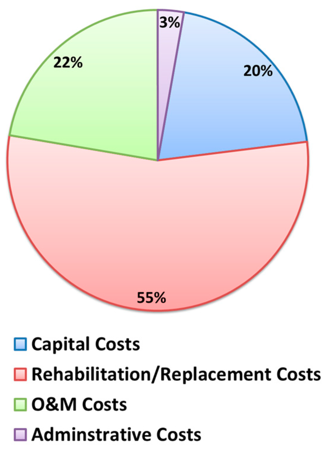
The cost components considered in the calculation of life cycle cost of a project are shown in Table 3. Capital costs occur in the first year when the stormwater control is installed. The rehabilitation or replacement costs occur every few years depending on type and size of BMP and location of project. The O&M costs occur annually throughout the life of the BMP [50]. Present value is used to compare scenarios with respect to total cost. An example of how the capital, the O&M, and the rehabilitation costs are distributed over time is shown in Figure 7. Also, an example of the distribution total cost into capital, O&M, rehabilitation, and administrative costs during the lifetime of project is shown in Figure 8. Equation (18) is used to calculate the total cost and Equation (19) is used to calculate present value.
BMP construction cost is calculated as:
C o n s t r u c t i o n   c o s t = α V β
where V is BMP volume, α and β are coefficients that vary with BMP type [48]. Capital cost is calculated as:
C a p i t a l   c o s t = C o n s t r u c t i o n   c o s t + L a n d   c o s t + C o s t   c o n t i n g e n c y
Land cost is a user input and cost contingency is calculated as a percentage of the construction cost.
The total cost is given by:
T o t a l   c o s t = C a p i t a l   c o s t + O & M   c o s t + R e h a b i l i t a t i o n   c o s t + A d m i n i s t r a t i v e   c o s t
O&M and administrative costs are also estimated as a percentage of the construction cost.
The tool calculates present value (PV) for a series of capital, O&M and rehabilitation costs occurring at different time periods during the lifetime of the project. PV for the lifetime of project is calculated based on total cost and discount rate.
P V = i = 1 n T C i × ( 1 + d i s c o u n t   r a t e ) i
where i refers to the year number and n is the lifetime of project in years.
T C i is total cost for the ith year, calculated as:
T C i = T o t a l   c o s t i × ( 1 + i n f l a t i o n   r a t e ) i
Capital costs are subject to financing costs and consist primarily of land, construction and contingency costs [48]. The construction costs for each BMP is calculated as a function of BMP size and adjusted for year and location of construction based on the Engineering News-Record (ENR) construction cost index database. A summary of cost categories is shown in Table 3.

4. Verification of Component Modules

The section includes verification of component modules presented in Section 3 including hydrology module and BMP sizing modules using field observations. The section also includes evaluation of scenarios for BMP selection module.

4.1. Hydrology Module

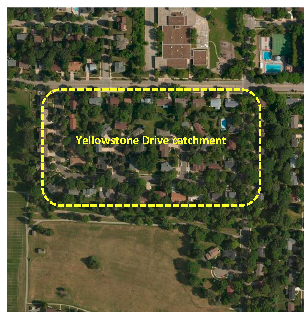
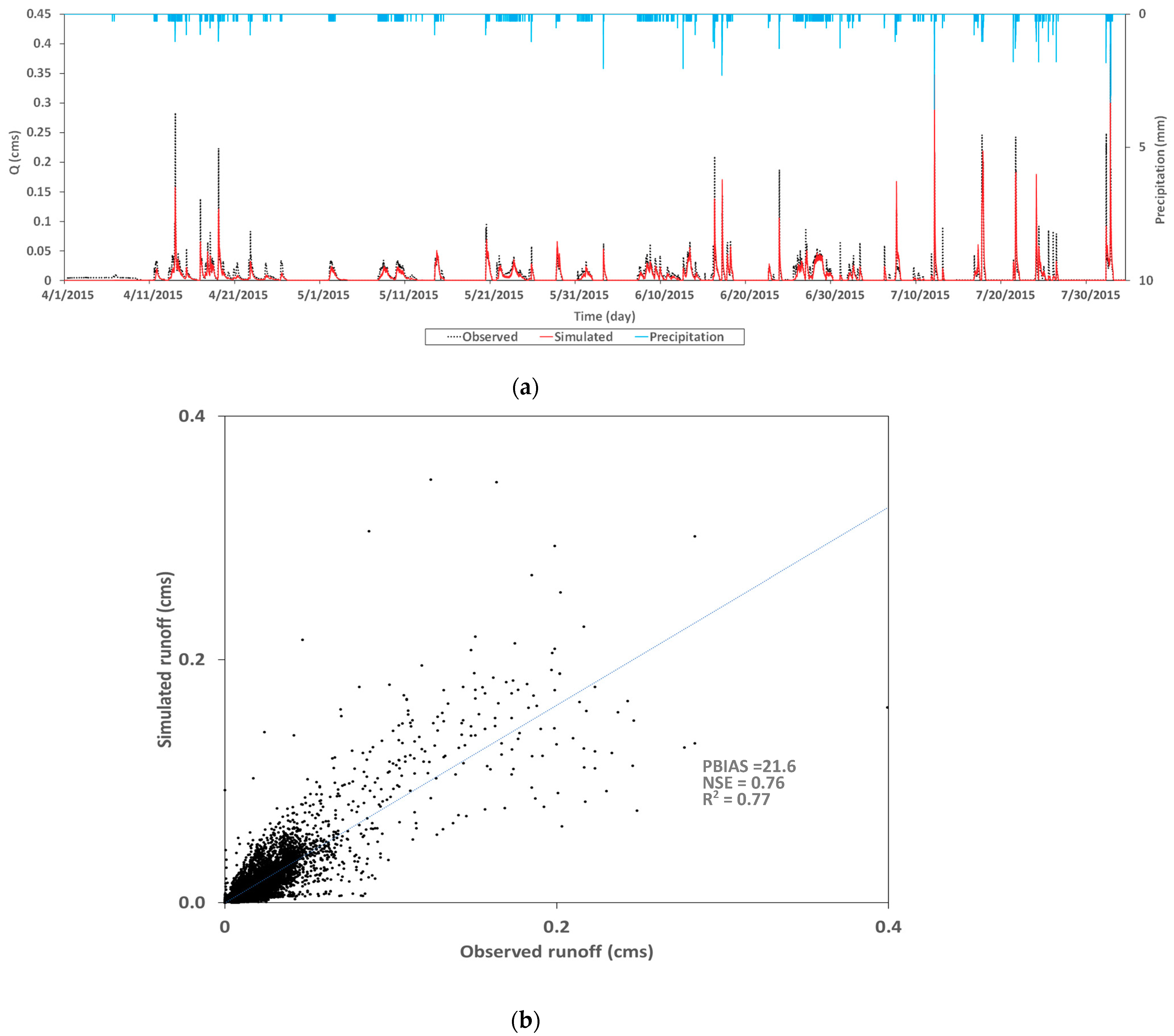
The outputs from the hydrology module were compared to observed data from a 6.4 ha catchment in Yellowstone Drive in Madison, Wisconsin [51]. Plan view of Yellowstone Drive catchment in Madison, Wisconsin is shown Figure 9. Percentage of area under various land cover types in Yellowstone Drive catchment is shown in Table 4. Precipitation data for a period of 4 months at one-minute time interval was obtained. The comparison of observed and simulated hydrograph for the site is shown in Figure 10.
Most papers discussing calibration of watershed models (e.g., [52,53]) use the coefficient of determination, R2, to measure the quality of calibration, which describes the degree of co-linearity between simulated and observed values and varies from 0 to 1. The model fit obtained in this work is relatively good (R2 = 0.77) given that R2 values greater than 0.5 are considered acceptable [54]. Although R2 has been widely used for model evaluation, this statistic is oversensitive to outliers and insensitive to additive and proportional differences between simulated values and observed data [55]. Hence, measures such as the Nash–Sutcliffe coefficient of efficiency (NSE) [56] and Root Mean Square Error (RMSE) are often considered to be more appropriate [57]. Thus, the NSE was also calculated. The limitation of NSE is that it does not include weighting, thus ignores differences in uncertainty in observations [58]. NSE determines the model efficiency as a fraction of the observed flow variance reproduced by the model as:
NSE = 1 i = 1 n ( S i O i ) 2 i = 1 n ( O i O M e a n ) 2
where O i is observed flow, S i is simulated flow, and O M e a n is observed mean flow.
Also, percent bias (PBIAS) was calculated which measures the average tendency of the simulated data to be larger or smaller than observed counterparts which has been applied in hydrology related research for evaluation of models [59]. PBIAS can vary between small and large values, both negative and positive, and by definition PBIAS values close to zero indicate better model performance and can be calculated as:
PBIAS = i = 1 n ( O i S i ) i = 1 n O i × 100
Based on Moriasi et al. [59], a PBIAS value of less than ± 25 and greater than ± 10 represents “satisfactory” model performance. Moriasi et al. [59] recommend that NSE value in the range of 0.6 and 0.8 represents “good” model performance.
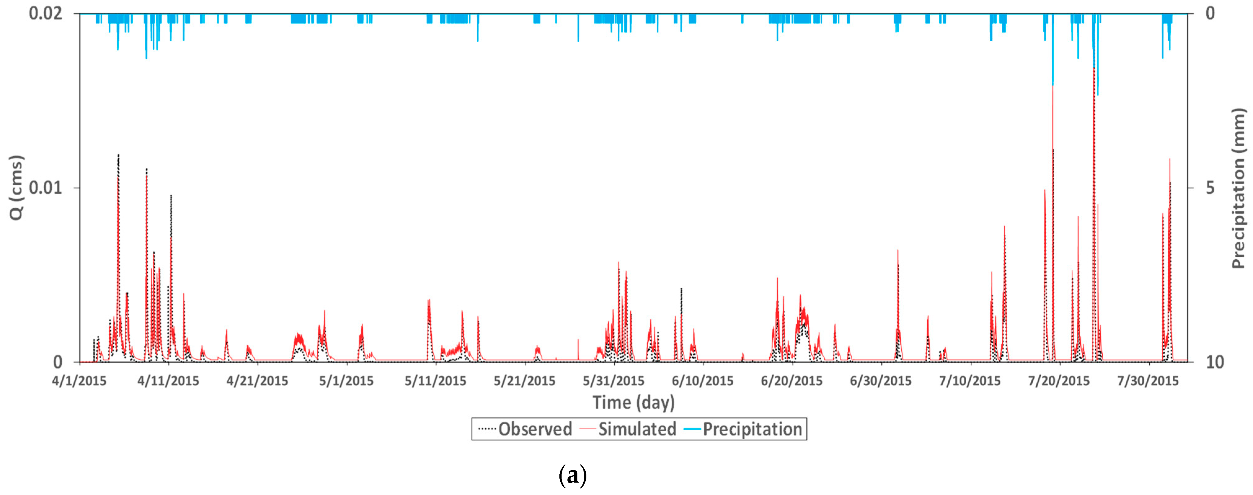
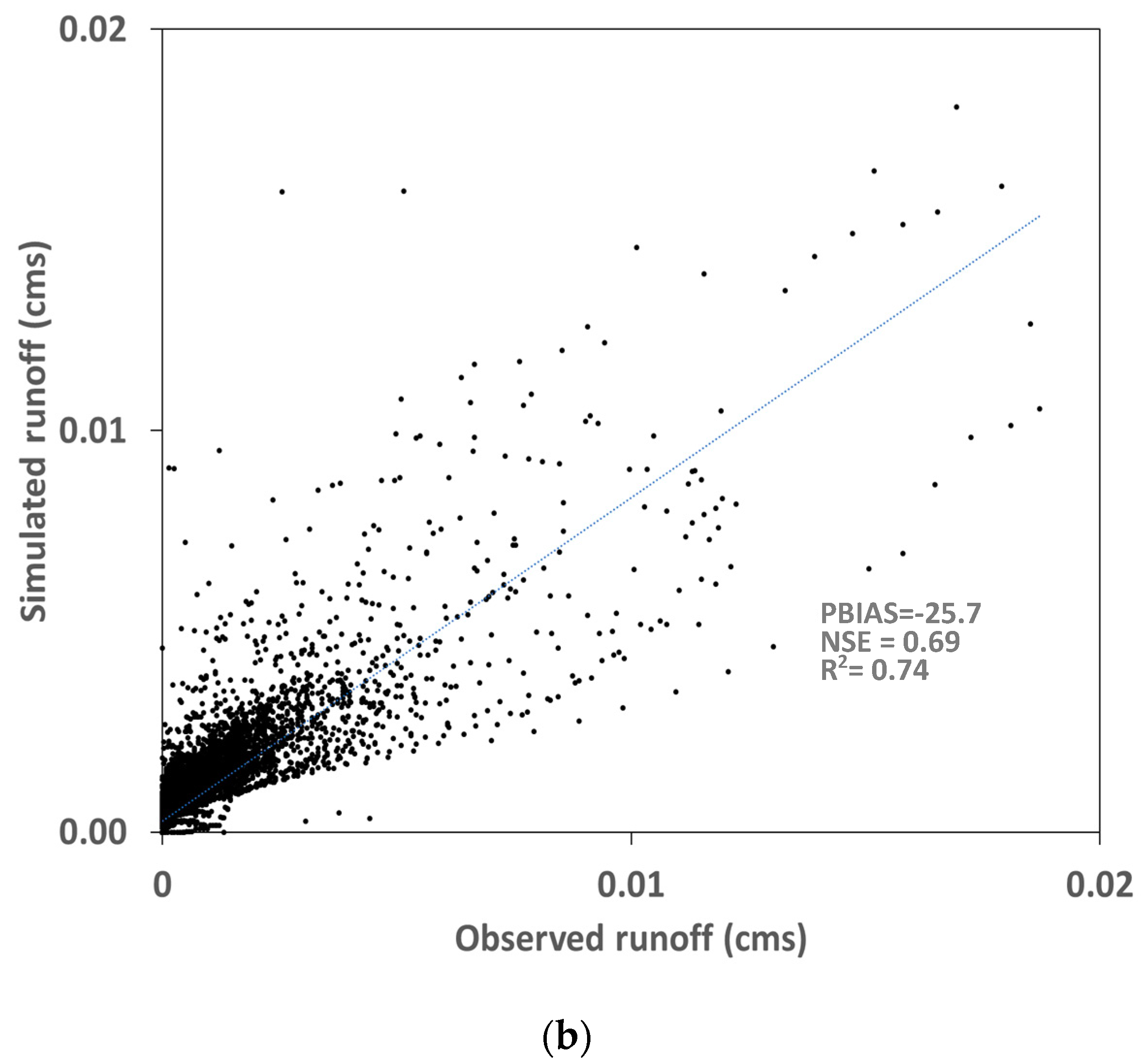
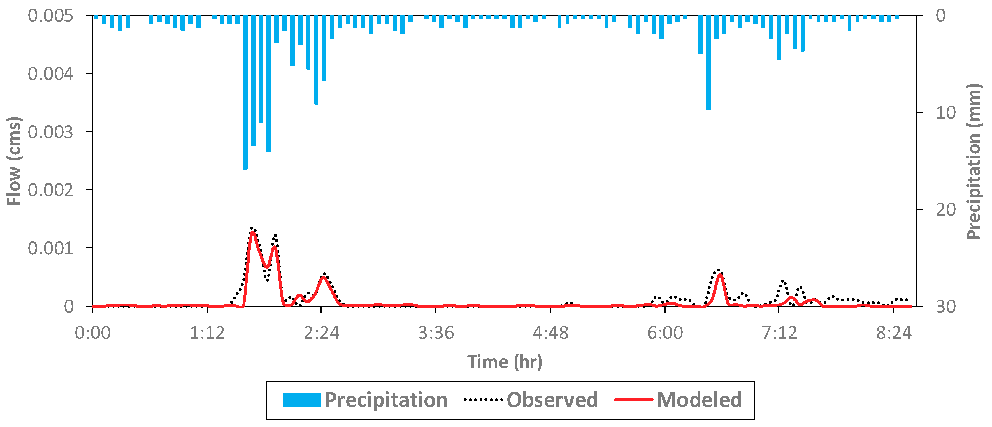
The hydrology module was also tested for an additional location; a small 1324 m2 parking lot in Madison, Wisconsin [51]. The comparison of observed and simulated output for the site is shown in Figure 11.

4.2. BMP Selection Scenario Analysis

To test the BMP selection module, the tool was tested for south east NCDC climate region for different scenarios, including land use types (Freeways, Residential, and Industrial) and pollutant concentration levels (minimum, median, and maximum concentration values) resulting in different inflow water quality. The results of BMP scenario analysis are presented in Table 5, Table 6 and Table 7. As stated earlier, the BMP removal efficiency data is obtained from the international stormwater BMP database [41]. Table 5, Table 6 and Table 7 to show summary of land use types, pollutant concentration levels, input water quality corresponding to the land use type and pollutant concentration level, and the BMP type selected by the module. The results from the BMP selection module for a residential land use for different input water quality based on minimum, median and maximum concentration form the BMP database are shown in Table 5. The tool selected rain garden for the minimum inflow concentration case, a bioretention for median concentration, and a combination of pretreatment and a bioretention for the maximum inflow concentration (a vegetated filter strip (VFS) combined with a bioretention) to meet required removal efficiency. The BMP selection module was tested for a second scenario in Table 6; an industrial land use for the minimum, median and maximum concentration levels. For industrial land use with minimum and median level of concentrations, the tool selected a wetland and a combination of BMPs (a forebay and a wetland) when a maximum concentration level was used.
The tool was also tested for a freeways land use option under the three concentration levels. As shown in Table 7, for the minimum and median concentration levels, a grass swale was selected. The tool selected the same BMP but with a forebay as pretreatment to meet the required removal efficiency for the maximum concentration level. The tool selected the same BMP for the minimum and median concentration levels (a wetland and grass swale) for some of the scenarios (e.g., industrial and freeways land use options). This suggests that the wetland and grass swale options meet the target concentration levels for both concentration levels (minimum and median). In both cases, the BMP selection changed to a combination of BMPs when the input concentration was changed to a maximum concentration. This suggests that the tool will select a relatively expensive BMP combination option only if the inflow concentration exceeds some threshold.
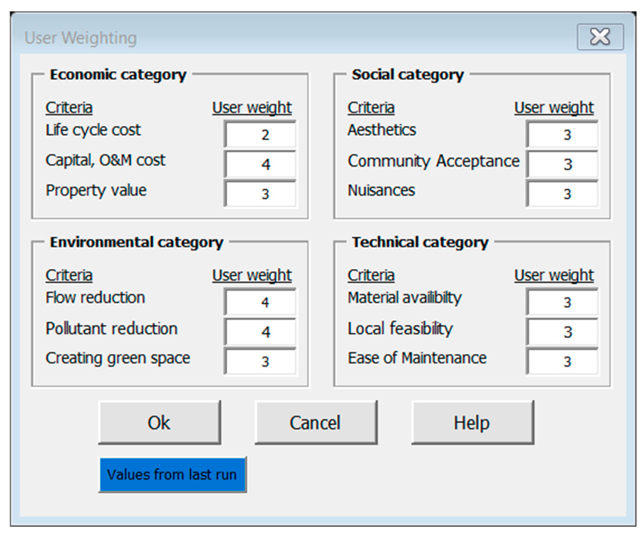
Default weighting values were used for all criteria described in Table 2. The default weights assigned to each criterion are shown in Figure 12. The tool allows users to change weights assigned to each criterion. If the user changes the weights assigned to each criterion, the BMP selection module may select another BMP or combination of BMPs. As discussed earlier, meeting target water quality is the driving factor in the BMP selection process. If multiple BMPs meet the target water quality requirement, the optimal BMP type with respect to all criteria will be selected. If cost is the only criterion, a relatively low cost BMP that meets the target water quality requirement is selected.

4.3. BMP Sizing Module

4.3.1. Green Roof System

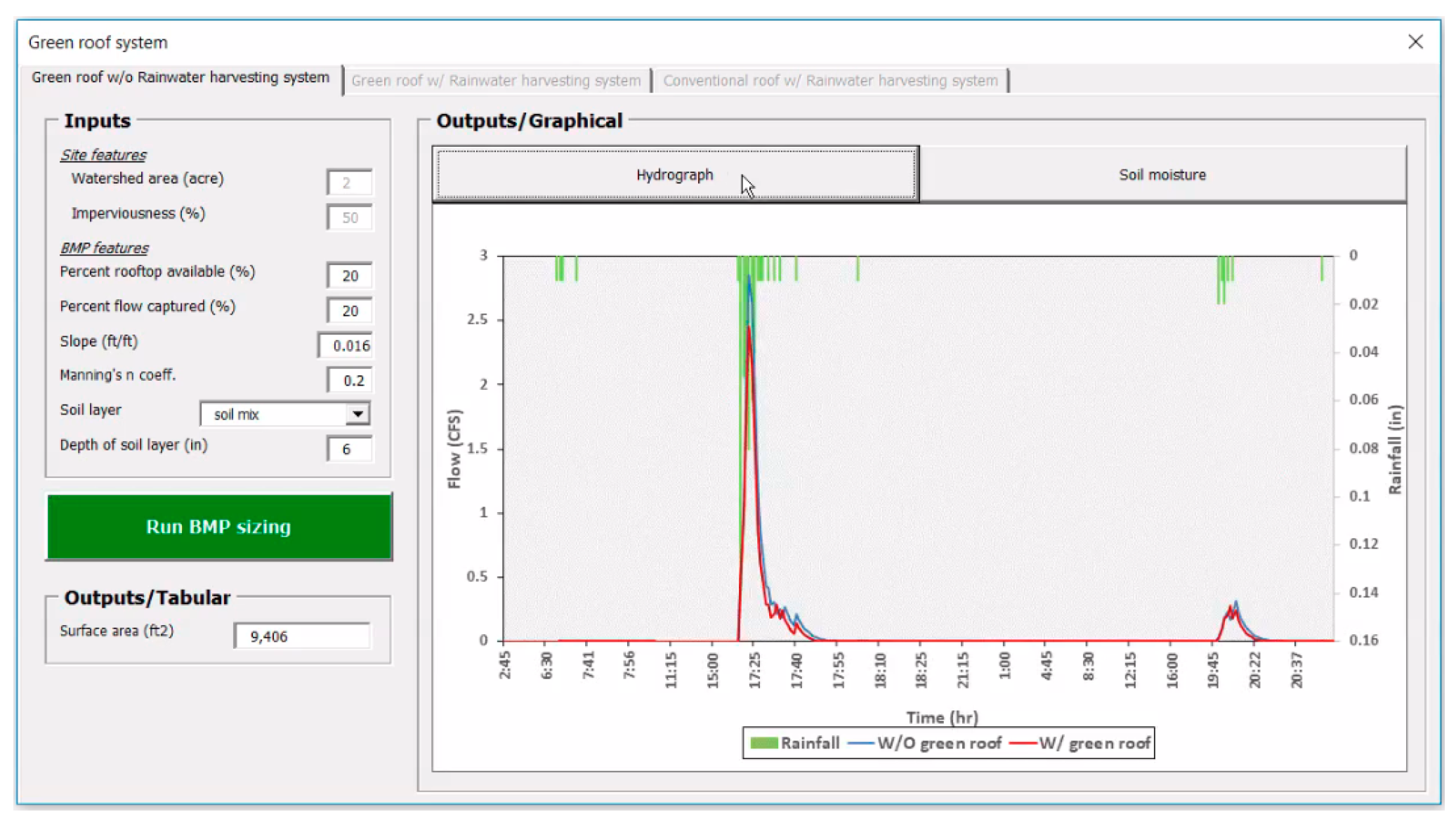
The output from green roof model was compared to observed data from South Dakota School of Mines research site. The results are shown in Figure 13. It was demonstrated that the green roof model within i-DSTss captured runoff patterns from a smaller size green roof with an area of 3 square meter (Figure 14).

4.3.2. Infiltration-Based BMPs

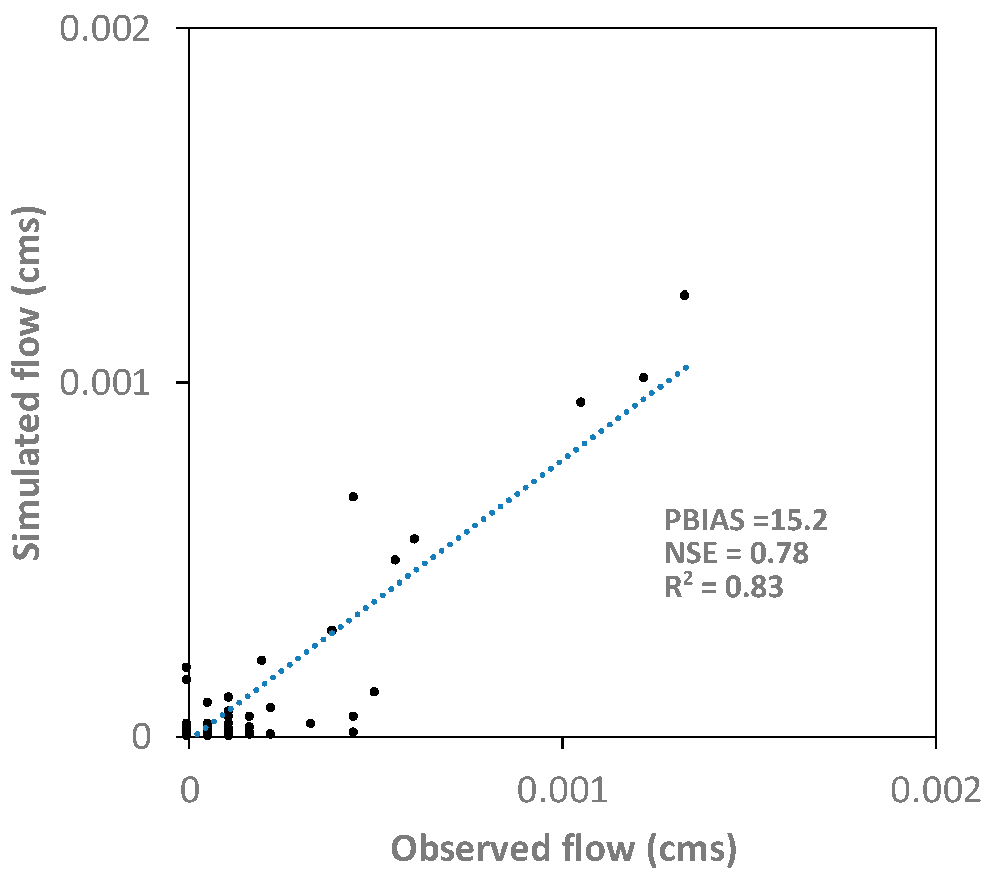
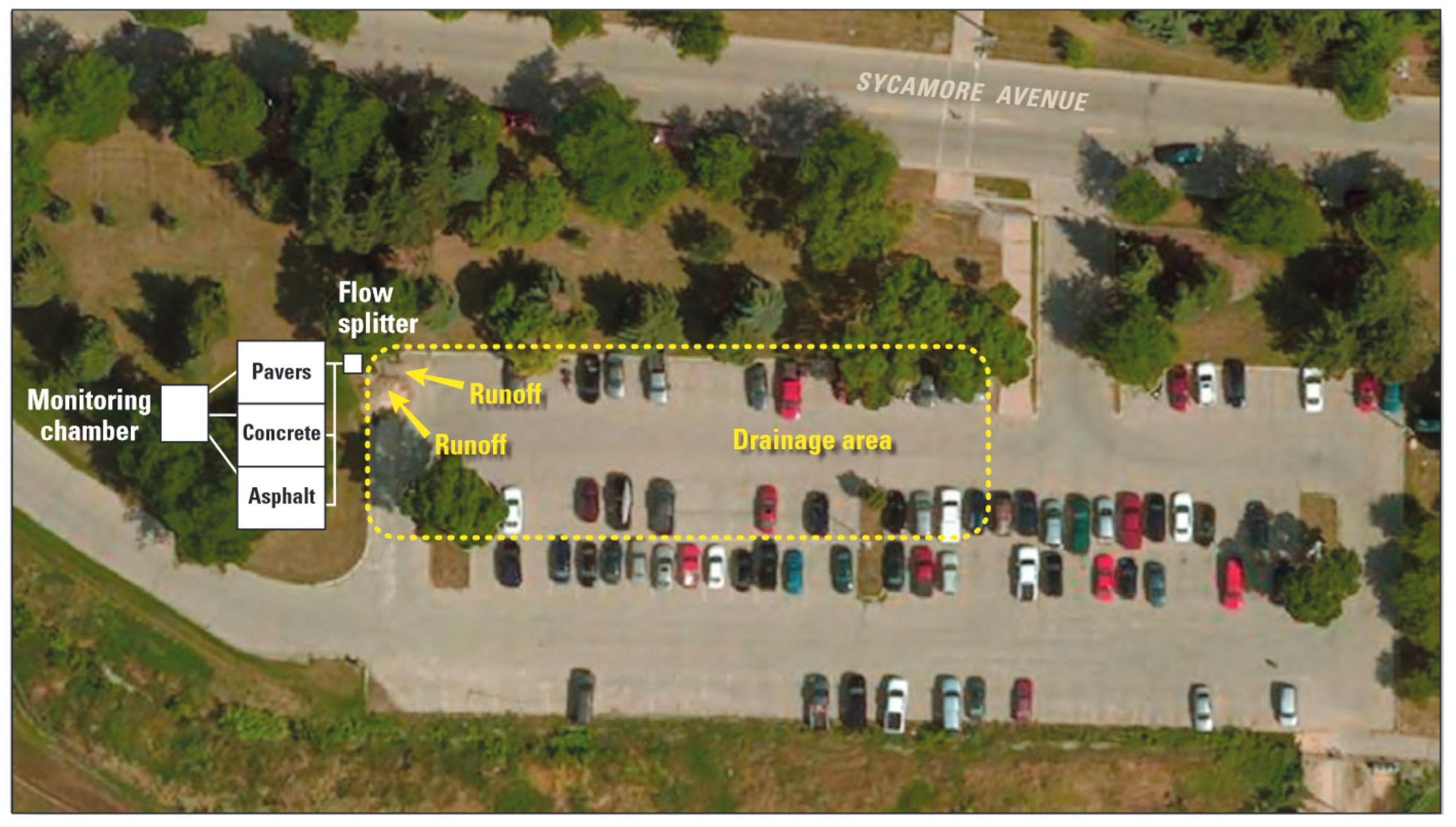
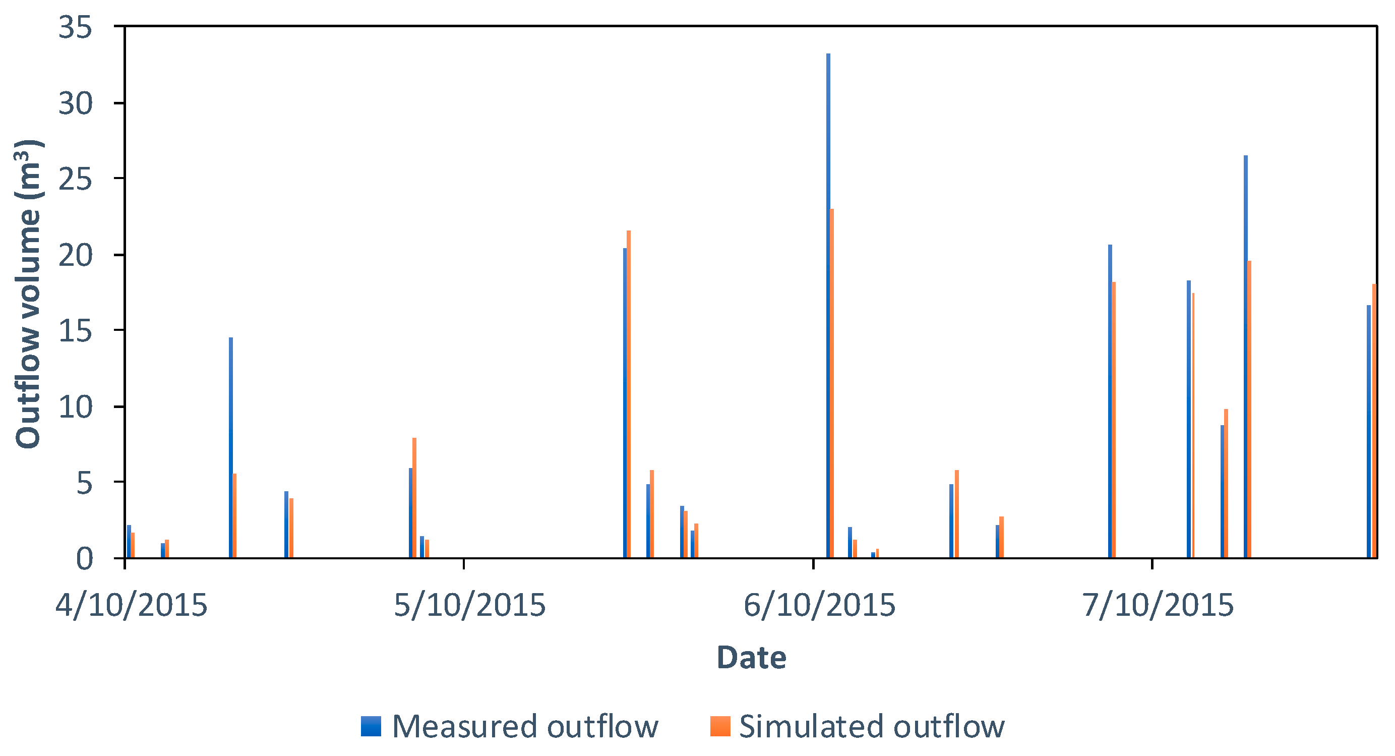
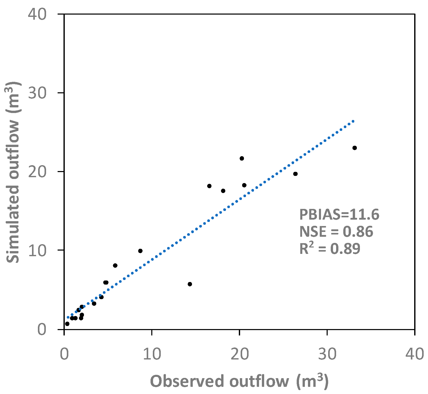
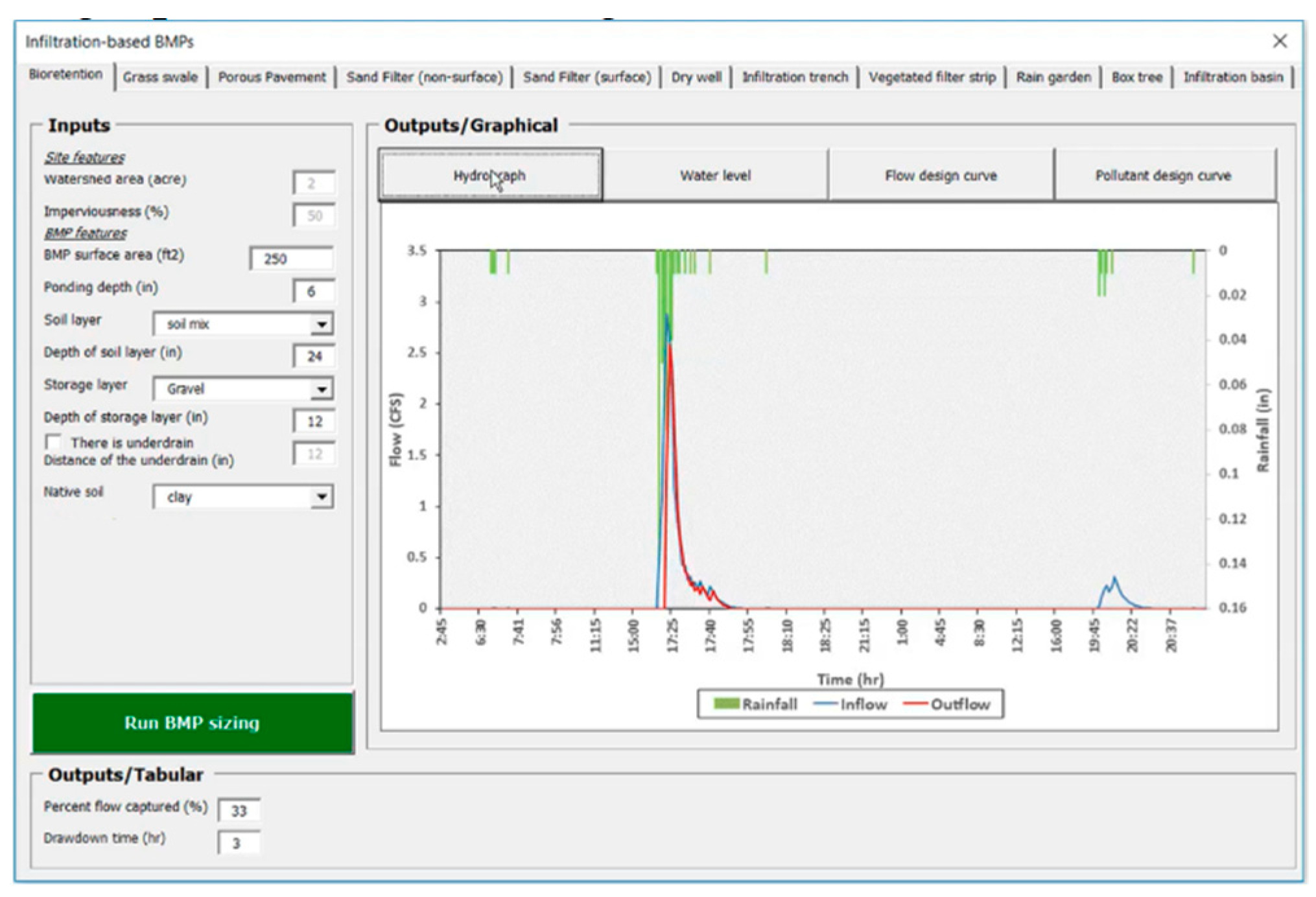
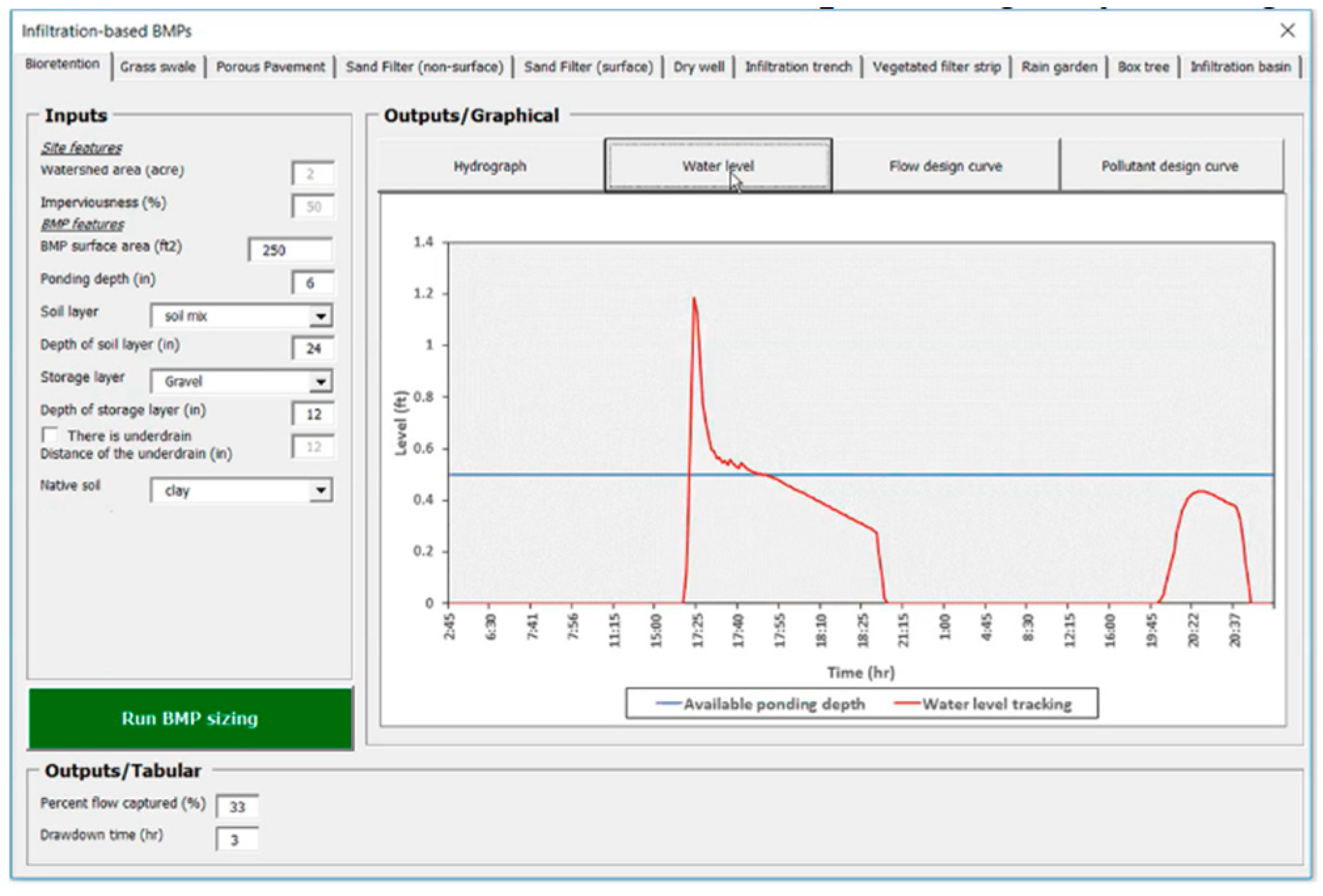
To demonstrate the performance of Infiltration-based BMPs, we used data from a permeable pavement LID practices. The parking lot area in Madison, Wisconsin with permeable pavement at the outlet of the parking lot is shown in Figure 15. Inflow and outflow volumes were measured for different events [60]. A comparison of measured and simulated outflow volumes is shown in Figure 16. The authenticity of the tool was assessed based on comparison of simulated and measure outflow. Statistical evaluation techniques including R2, NSE and PBIAS were used as performance measures.
R2, NSE, and PBIAS values for observed and simulated volumes from the permeable pavement are shown in Figure 17.

4.3.3. Storage-Based BMPs

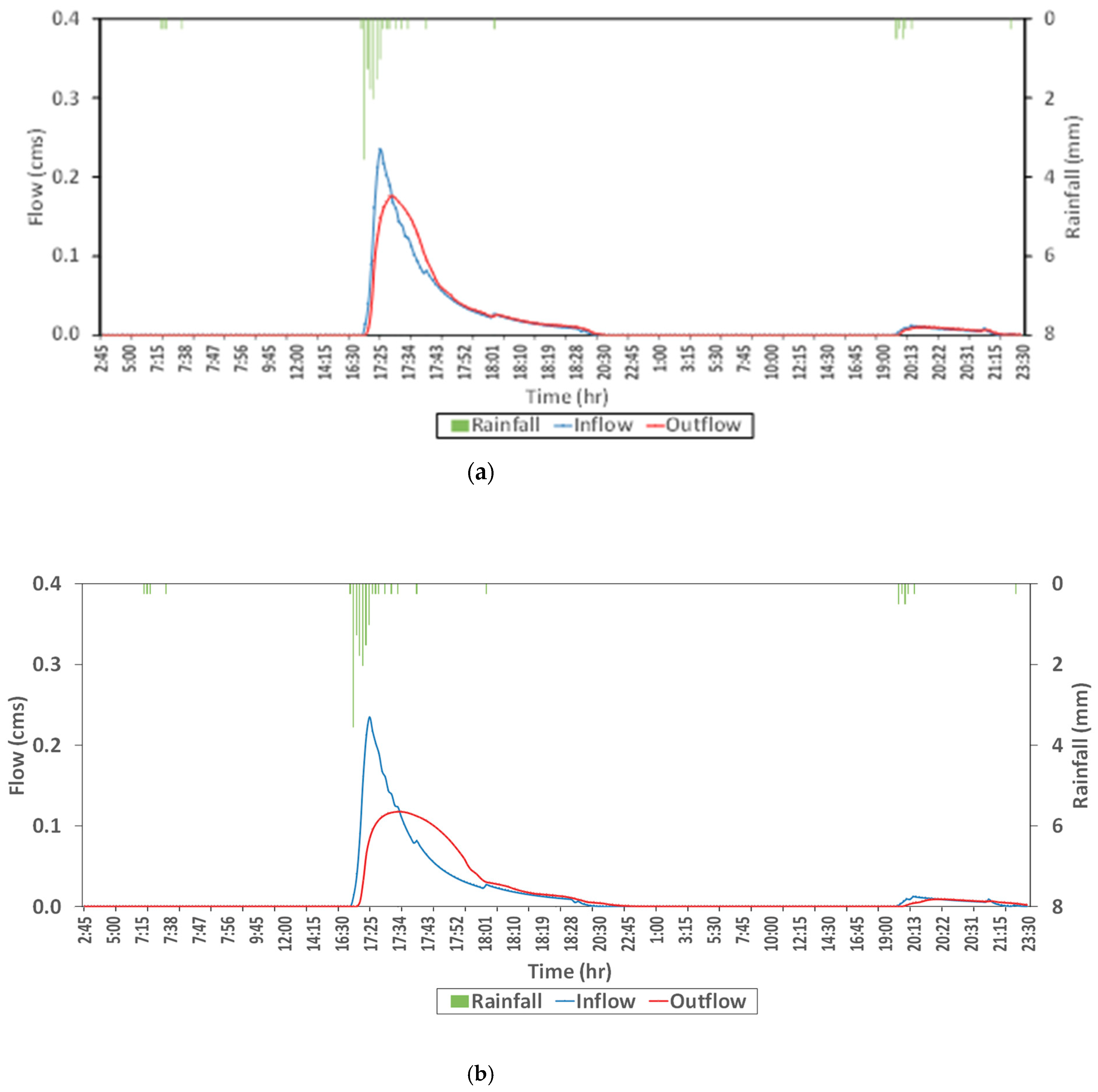
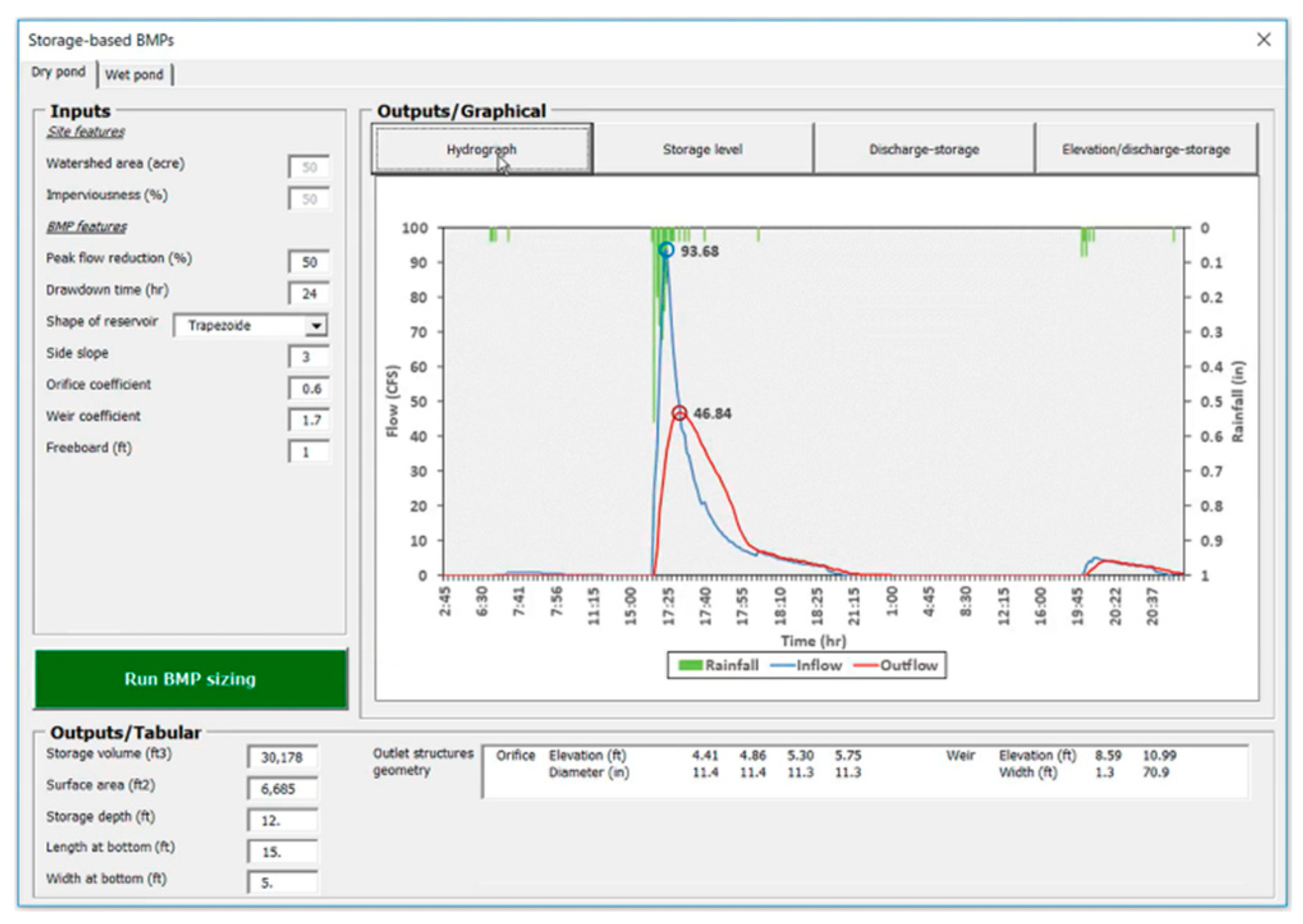
Two different scenarios are presented to demonstrate the storage-based BMPs. The results are presented in Figure 18 and Table 8. Inflow and outflow hydrograph for dry detention pond for 25 and 50 percent peak flow reduction as shown in Figure 18a,b respectively. The peak flow dropped from 0.23 cms to 0.17 cms and 0.11 cms for 25 and 50 percent peak flow reduction respectively. These hydrographs have been generated from a watershed with area of 8.1 hectare and 50 percent imperviousness and precipitation time series also shown in Figure 18. Summary of outputs for two different scenarios is shown in Table 8. Also, the change in percent of peak flow reduction and corresponding change in pond volume, depth and bottom width is shown in Table 8.

5. The User Interface

The user interface design and the level of interactivity are important factors to enable broader use of any decision support tool. A user interface should facilitate easy quantitative data input and allow user intervention to change alternatives [61]. Usually, little attention is given to the user interface when a decision support tool is intended as a conceptual demonstration or evaluation of approaches [62], or when it is intended for a highly specific use, or for expert users who are more concerned with the theory behind the decision process [63,64]. This i-DSTss tool is intended to be used by a wide range of utilities, and/or by users who may not be modelers, and therefore employs a user interface that allows easy interaction. Interactivity can be in the form of data inputting, ability to monitor the decision process, and/or changing constraints or rules that reflect the user’s preferences or giving a warning message if any design standards are violated [42,65,66]. It is important that the user interface integrates the various underlying modules. The organization of the graphical user interface is shown in Figure 19. The user will be able to modify the inputs for different modules including runoff, water quality, removal efficiency, BMP sizing, and cost analysis as shown in Figure 19. Within each input, the user has the ability to change and modify the various factors that affect the outcomes. User can then run i-DSTss and visualize the outputs also from the user interface.

6. Conclusions

The i-DSTss tool integrates several modules, including hydrology, BMP selection, BMP sizing and cost. Decision support tools in stormwater management become more useful to the users when they integrate multiple criteria and objective functions. The i-DSTss includes technical, environmental, social and economic criteria in the BMP selection module. The graphical user interface allows altering constraints that may result in a different type and size of BMP. To assess the authenticity of the tool, prediction from the tool for each module type (hydrology and sizing) were compared with observed data and the goodness-of-fit was evaluated in each case. The hydrology module predicted runoff from small residential area and a parking lot with R2 and NSE values greater than 0.7 in each case. The BMP sizing module includes sizing options for green roofs, infiltration-based BMPs and storage-based BMPs. The tool predicted outflow rate from a permeable pavement with R2 and NSE values greater than 0.8. It was demonstrated through scenario evaluation that the BMP selection module recommended cost effective BMPs. A significant merit of the tool is that complex approaches were translated into easy to use, computationally less intensive, yet rigorous physically based modules that could be verified with observations. The tool can aid decision makers in analyzing various stormwater scenarios at the site-scale level.

Author Contributions

Conceptualization, A.S., M.G., J.M., T.S.H; methodology, A.S., M.G.; investigation, A.S., M.G.; development, A.S.; writing—original draft preparation, A.S., M.G.; writing—review and editing, A.S., M.G., J.M., T.S.H; supervision, M.G.; project administration, T.S.H.

Funding

This work was supported by the Environmental Protection Agency (EPA) [grant number EPA-G2015ORD-D1].

Acknowledgments

We acknowledge William Selbig and USGS for sharing hydrologic data from Yellowstone Drive catchment and parking lot in Madison, Wisconsin. Jason Philips from South Dakota School of Mines and Technology provided hydrology data for the green roof.

Conflicts of Interest

The authors declare no conflict of interest

Appendix A. Detailed Procedures

In this section detailed procedures for the various modules in the i-DSTss framework (hydrology module, BMP selection module, and BMP sizing module) are provided.

Appendix A1. Hydrology Module

The hydrology module includes event and continuous simulation methods for calculating runoff from precipitation time series. The Green-Ampt and Curve Number methods are used for runoff calculation. In both Green-Ampt and Curve Number methods, the runoff depth is calculated using a mass balance approach considering precipitation intensity (i), evapotranspiration rate (e), and infiltration rate (f). The runoff depth is used to calculate overland flow.

Appendix A1.1. Green-Ampt Method:

The following steps are used to calculate runoff.
  • Step 1: Calculate precipitation intensity, i (mm/h)
    i = P Δ t
    where P (mm) is incremental precipitation, Δ t   ( h ) = t i + 1 t i is time step and i (mm/h) is precipitation intensity.
  • Step 2: Calculate cumulative infiltration, F t   ( mm ) [37]
    F t = Ψ × I M D × { 1 [ t * + ln [ 1 + t * + 2 t * ( 1 + 2 t * / 6 ) ] 1 1 + t * + 2 t * ( 1 + 2 t * / 6 ) 1 ] }
    where t * = K s × Δ t Ψ × I M D , K s ( mm / h ) is saturated hydraulic conductivity, Ψ (mm) is suction head, IMD is initial soil moisture deficit calculated as:
    I M D = θ s θ i
    where θ s and θ i are saturated and initial soil water content respectively.
The cumulative infiltration, Ft at time t depends on initial soil moisture deficit (IMD), and other soil physical properties such as suction head (ψ), and saturate hydraulic conductivity (Ks). Higher IMD and ψ values suggest a higher cumulative infiltration Ft at time t.
  • Step 3: Calculate infiltration rate, f   ( mm / h ) [32]
    f = K s ( 1 + Ψ × I M D F t )
The infiltration rate depends on cumulative amount that has already infiltrated calculated in Step 2, initial soil moisture deficit, suction head, and saturated hydraulic conductivity. The initial moisture deficit (IMD) is important parameter for calculation of the cumulative infiltration (Ft), and infiltration rate (f). Thus, IMD has to be updated each time step based on water input to account for the effect of IMD on infiltration rate. Equation for updating IMD is given in Step 4 below.
  • Step 4: Update soil moisture account [20]
The soil moisture is updated every time step to account for the effect of soil moisture condition on infiltration and runoff.
The soil moisture is continuously updated depending on whether there is precipitation input or not.
  • Case 1: If there is precipitation input (P ≠ 0), the soil moisture deficit (IMD) is updated using Equation (A5) below.
    I M D t i = M a x ( I M D t i 1 f × Δ t 4 K s , 0 )
    where I M D t i is the soil moisture deficit at the end of a time step and I M D t i 1 is the soil moisture deficit at beginning of the time step.
Equation (A5) suggests that the soil moisture deficit at the end of a time step is a function of the soil moisture deficit at beginning of the time step, amount infiltrated during time step (Δt), f × Δt, and the saturated hydraulic conductivity of the soil.
  • Case 2: If there is no precipitation input (P = 0), then the soil moisture deficit (IMD) is updated using Equation (A6) below.
    I M D t i = M i n ( I M D t i 1 + I M D m a x × K r × Δ t , θ s θ r )
    where θ r is residual soil water content, and K r   ( h ) is moisture deficit recovery constant calculated as: K r   ( h 1 ) = K s ( mm / h ) 2.95 .
The moisture deficit recovery constant (Kr) is a parameter that describes how fast the soil moisture changes in the absence of precipitation input and it is dependent on saturate hydraulic conductivity of the soil.
  • Step 5: Calculate evapotranspiration
The evapotranspiration is calculated using Hargreaves equation [34]
E T = 0.023 ( 0.408 ) ( T m e a n + 17.8 ) ( T m a x T m i n ) 0.5 R a
where Tmax = maximum air temperature (°C), Tmin = minimum air temperature (°C), Ra = extraterrestrial radiation (MJ·m−2), and 0.408 is a unit conversion factor. Extraterrestrial radiation, Ra, is estimated based on latitude and the calendar day of the year given as:
R a = 24 × 60 π G s c d r [ ω s sin ( φ ) sin ( δ ) + cos ( φ ) cos ( δ ) sin ( ω s ) ]
where Gsc = solar constant (0.0820 MJ·m−2·min−1), φ = latitude (radians), converted from degrees latitude to radians (radians = degrees(π/180)), and the term 24 × 60 is a factor to convert minute to day.
The remaining parameters are determined based on the calendar day of the year:
d r = 1 + 0.33 cos ( 2 π 365 J )
where d r = inverse relative distance from earth to sun, and J = calendar day of the year,
δ = 0.409 sin ( 2 π 365 J 1.39 )
ω s = cos 1 ( tan ( φ ) tan ( δ ) )
where δ = solar declination (radians), and ω s = sunset hour angle (radians).
The initial version of Hargreaves equation for evapotranspiration is based on daily time steps. The equation was modified to disaggregate the daily evapotranspiration estimates into sub-hourly estimates using a cosine function given by [35,36]:
e = E T × ( 0.1302 × Δ t × cos ( 2 π × ( 11.23 + t ) 24 ) )
where Δ t is time step (h) and t is cumulative time (h).
  • Step 6: Calculate the rainfall excess i *
The rainfall excess i * is calculated using precipitation intensity, infiltration and evapotranspiration rates calculated in steps 1, 3, and 5.
i * p e r v i o u s = i f e
i * i m p e r v i o u s = i e
where i * p e r v i o u s is rainfall excess from pervious area and i * i m p e r v i o u s is rainfall excess from impervious area.
  • Step 7: Calculate ponding depth [20]
The rainfall excess i * represents part of the precipitation input available for surface ponding and runoff. A fraction of the surface ponding, obtained after deducting depression storage, is available for runoff. This faction of surface ponding is used to calculate runoff amount. The runoff amount is estimated using Manning’s equation.
d D d t = i * w × s 1 2 A × n ( D d p ) 5 3
Equation (A15) is implicit and requires iteration to calculate D (surface ponding depth). The equation was transformed into explicit form by converting the exponential equation to a quadratic equation as described in [39]:
D 5 3 = a D 2 + b D + c
where a = 0.730, b = 0.292, and c = 0.0146
d D d t = i * + W C O N ( D d p ) 5 3
D t i + 1 D t i Δ t = i * + W C O N ( D t i + 1 2 ( D t i + 1 D t i ) d p ) 5 3
If D t i + 1 D t i = x , we have:
x = i * × Δ t + W C O N × Δ t × ( 1 2 x + ( D t i d p ) ) 5 3
x = i * × Δ t + W C O N × Δ t × { a × ( 1 2 x + ( D t i d p ) ) 2 + b × ( 1 2 x + ( D t i d p ) ) + c }
x = i * × Δ t + W C O N × Δ t × { a × ( 1 4 x 2 + x ( D t i d p ) + ( D t i d p ) 2 ) + b × ( 1 2 x + ( D t i d p ) ) + c }
Equation (A21) can be rearranged into a quadratic form ( A x 2 + B x + C = 0 ) as:
{ a × W C O N × Δ t 4 } x 2 + { a × W C O N × Δ t × ( D t i d p ) 1 + b 2 × W C O N × Δ t } x + { a × W C O N × Δ t × ( D t i d p ) 2 + b × W C O N × Δ t × ( D t i d p ) + c × W C O N × Δ t + i * × Δ t } = 0
Then D t i + 1 can be calculated using the expression x = B ± B 2 4 A C 2 A as:
For pervious area A, B and C are given by:
A = a × W C O N p e r v i o u s × Δ t 4
B = a × W C O N p e r v i o u s × Δ t × ( D t i d p , p e r v i o u s ) 1 + b 2 × W C O N p e r v i o u s × Δ t
C = a × W C O N p e r v i o u s × Δ t × ( D t i d p , p e r v i o u s ) 2 + b × W C O N p e r v i o u s × Δ t × ( D t i d p , p e r v i o u s ) + c × W C O N p e r v i o u s × Δ t + i * × Δ t
For impervious area A, B and C are given by:
A = a × W C O N i m p e r v i o u s × Δ t 4
B = a × W C O N i m p e r v i o u s × Δ t × ( D t i d p , i m p e r v i o u s ) 1 + b 2 × W C O N i m p e r v i o u s × Δ t
C = a × W C O N i m p e r v i o u s × Δ t × ( D t i d p , i m p e r v i o u s ) 2 + b × W C O N i m p e r v i o u s × Δ t × ( D t i d p , i m p e r v i o u s ) + c × W C O N i m p e r v i o u s × Δ t + i * × Δ t
Where W C O N p e r v i o u s = W S 1 / 2 A p e r v i o u s × n p e r v i o u s , W C O N i m p e r v i o u s = W S 1 / 2 A i m p e r v i o u s × n i m p e r v i o u s
  • Step 8: Calculate overland flow/runoff [20]
After calculation of runoff depth in Step 7, overland flows are calculated separately for pervious and impervious areas using Equations (A29), (A30) below.
Q = Q p e r v i o u s   a r e a + Q i m p e r v i o u s   a r e a
Q = 1 n p e r v i o u s × W × %   p e r v i o u s × ( D t i + 1 d p p e r v i o u s ) 5 3 × S 1 2 +
1 n i m p e r v i o u s × W × %   i m p e r v i o u s × ( D t i + 1 d p i m p e r v i o u s ) 5 3 × S 1 2
where d p p e r v i o u s , n p e r v i o u s are depression storage and Manning’s coefficient for pervious area and d p i m p e r v i o u s , n i m p e r v i o u s are depression storage and Manning’s coefficient for impervious area. W and S are width and slope of watershed respectively.

Appendix A1.2. Curve Number Method:

Similar to the Green-Ampt approach, overland flow is calculated using a mass balance approach considering precipitation intensity (i), evapotranspiration rate (e), and infiltration rate (f).
  • Step 1: Calculate precipitation intensity, i (mm/h)
    i = P Δ t
  • Step 2: Calculate cumulative infiltration F (mm) [20]
    F = p p 2 p + S
    where p (mm) is cumulative precipitation and S is retention parameter calculated as [33]:
    S = 1000 C N c o m p o s i t e 10
    where C N c o m p o s i t e is composite Curve Number calculated using Equation (A34) below.
    C N c o m p o s i t e = i = 1 n C N i × A i i = 1 n A i
    where C N i ,   A i are Curve Number and area for ith segment respectively and n is number of total segments.
  • Step 3: Calculate infiltration rate f (mm/h)
    f = F t i + 1 F t i Δ t
  • Step 4: Update retention parameter [20]
For event simulation, a constant value is used for the retention parameter. For continuous simulation, the retention parameter is updated depending on whether there is precipitation input or not to account for the effect of soil moisture content on infiltration (Note: The updated S is used to calculate F).
  • Case 1: If there is precipitation input (P ≠ 0), the retention parameter is updated using Equation (A36) below.
    S t i = M a x ( S t i 1 f × Δ t , S m i n )
Equation (A36) suggests that retention parameter value at end of the time step is a function of the retention parameter value at beginning of the time step and amount infiltrated during time step (Δt).
  • Case 2: If there is no precipitation input (P = 0), then the retention parameter is updated using Equation (A37) below.
    S t i = M i n ( S t i 1 + S m a x × K r × Δ t , S m a x )
Equation (A37) suggests that retention parameter value at end of the time step is a function of the retention parameter value at beginning of the time step, and moisture deficit recovery constant ( K r ) .
where:
S m i n = 1000 C N m a x 10
S m a x = 1000 C N m i n 10
where C N m a x is maximum Curve Number, and C N m i n is minimum Curve Number.
The methods for calculating evapotranspiration, runoff depth and overland flow are similar to the methods used in Green-Ampt approach discussed earlier.

Appendix A2. BMP Selection Module

The BMP selection module selects a BMP for site from a list of BMP built into the tool based on input water quality, target water quality, BMP efficiency, and other factors such as technical, economic, environmental and social criteria.

Appendix A2.1. Input Water Quality

Input water quality is obtained from national stormwater quality database (NSQD) based on NCDC climate region, land use and level of concentration [40].

Appendix A2.2. Target Water Quality

Target water quality requirements refers to water quality requirements for discharge or reuse which can be obtained from standards set by the U.S. Environmental Protection Agency (USEPA) or user input values.

Appendix A2.3. BMP Removal Efficiency

The BMP removal efficiencies are calculated based on input water quality concentration and target water quality using Equation (A40) below.
R e m o v a l   e f f i c i e n c y   r e q u i r e d   ( % ) = ( I n p u t   w a t e r   q u a l i t y T a r g e t   w a t e r   q u a l i t y ) I n p u t   w a t e r   q u a l i t y × 100
Then the calculated removal efficiencies are compared with BMP removal efficiency obtained from international stormwater BMP database [41]. A BMP with a removal efficiency greater than the calculated value is selected. Other criteria including economic, environmental and social are considered during the selection process. A multi-objective optimization procedure is used during the selection. Meeting the target water quality requirement is a priority in the selection process.

Appendix A3. BMP Sizing Module

For the purpose of BMP design, we categorized the BMPs in three different groups including green roof system, infiltration-based BMPs, and storage-based BMPs. Details about the sizing procedures for each BMP category is discussed below.

Appendix A3.1. Green-Roof System

A mass balance approach was applied for green roof system. The water input to the green roof system is precipitation. The losses include evapotranspiration, overflow, and underdrain. The difference between water input and the losses becomes change in storage. Thus, the rate of water input and loss is given by:
i E T U D O F = Δ θ Δ t d s o i l
where i is precipitation intensity (mm/h), ET is evapotranspiration rate (mm/h), UD is underdrain rate (mm/h), OF is overflow rate (mm/h), Δ t is time step (h), Δ θ is changing in soil moisture, and d s o i l is depth of soil/media (mm). Multiplying the rates by the time step we get:
P E T ' U D ' O F ' = Δ θ × d s o i l
where P is precipitation (mm), ET’ is evapotranspiration (mm), UD’ is underdrain (mm), and OF’ is overflow (mm). Overflow refers to part of the inflow that does not infiltrate or become underdrain discharged through an overflow system. Underdrain refers to flow that originates from gravity water held between field capacity and saturation.
ET’, UD’ and OF’ are calculated based on water content. ET’ includes transpiration from vegetation and evaporation from the land surface. We assumed transpiration does not occur if the soil moisture content is below the wilting point and at saturation. Evaporation occurs for all moisture conditions above the residual water content. Possible conditions for ET’, UD’ and OF’ calculation included in the model are:
  • I f   θ < θ W P no   transpiration   , E T ' = E T   c alculated   by   Hargreaves   Equation ,   O F ' = 0 ,   and   U D ' = 0
  • I f   θ W P θ θ F C E T = M i n ( E T   calculated   by   Hargreaves   Equation   and   ( θ θ W P ) × d s o i l ) ,   O F ' = 0 ,   and   U D ' = 0
  • I f   θ F C < θ < θ s E T = M i n ( E T   calculated   by   Hargreaves   Equation   and   ( θ F C θ W P ) × d s o i l ) ,   O F ' = 0   , and   U D ' = ( θ θ F C ) × d s o i l
  • I f   i > k s ,   θ = θ s   no   transpiration ,   E T = E T   calculated   by   by   Hargreaves   Equation O F = ( i k s ) × Δ t ,   and   U D ' = ( θ s θ F C ) × d s o i l
where θ is soil moisture content, θ W P is soil moisture content at wilting point, θ F C is soil moisture content at filed capacity point, θ s is soil moisture content at saturation, i is precipitation intensity, and ks is saturate hydraulic conductivity.

Updating water content of media:

The underdrain and overflow amounts are dependent on the water content of the media. Thus, the moisture content is updated every time step.
θ r θ t i + 1 = { P E T ' U D ' O F ' d s o i l + θ t i } θ s
Equation (A43) suggests that the soil moisture content ranges from residual moisture content ( θ r ) to saturated moisture content ( θ s ) .

Calculate runoff flow from green roof:

Q = Q O F ' + Q U D '
Q = 1.49 n w × s × ( O F ' ) 5 3 + K ( U D ' ) n
where k = 0.3, and n = 2

Appendix A3.2. Infiltration-Based BMPs

A mass-balance approach is used to determine overflow and underdrain rates. The inflow into BMPs includes precipitation over the surface area of the BMP and runoff from the drainage area. Outflow/loss from the BMP includes evapotranspiration and infiltration. The BMPs may have up to three layers (surface/ponding layer, a soil layer and a storage/gravel layer). The mass balance approach is applied for each layer.
The mass balance equations for each layer is given in following Equations (A46)–(A48):
Surface   layer :   P + R u n o f f E T I N F O F = Δ s 1 Δ t
where P is precipitation rate, Runoff is runoff calculated from hydrology module, INF is infiltration rate, ET is evapotranspiration rate, OF is overflow rate, Δ s 1 is changes in storage in surface layer, and Δ t is time step.
Soil   layer :   I N F E T ' P E R = Δ s 2 Δ t
where ET’ is evapotranspiration in soil layer, PER is percolation rates into a storage layer, and Δ s 2 is changes in storage in soil layer.
Storage   layer :   P E R P E R U D = Δ s 3 Δ t
where PER’ is percolation out of a storage layer and into a native soil, UD is underdrain rate, and Δ s 3 is changes in storage in storage/gravel layer.
Darcy’s principle is applied to calculate percolation rate in the soil and storage layer Equations (A47) and (A48).
  • i f   θ θ F C     P E R = 0 , this suggest that suction is greater than gravity and water is held tightly with the soil, thus, percolation does not occur.
  • i f   θ > θ F C     P E R = k s e H C O ( θ s θ ) where k s is saturated hydraulic conductivity, H C O is decay constant typically in the range of 5 to 15, θ s is soil moisture content at saturation, θ F C is soil moisture content at filed capacity, and θ is soil moisture content during the time interval [20].
Note that when θ > θ F C , gravity forces are greater than suction forces and water percolates downward (drainage occurs)
Drawdown time is the time that water captured by the BMP must drain. This time may range from 24 h to 48 h.
D r a w d o w n   t i m e   ( h ) = p o n d i n g   d e p t h i n f i l t r a t i o n   r a t e + θ × s o i l   d e p t h p e r c o l a t i o n   r a t e

Appendix A3.3. Storage-Based BMPs

Level pool routing method is implemented in i-DSTss. The level pool routing procedure is a method for calculating the water level (h) and outflow hydrograph given inflow hydrograph and storage-outflow characteristics. The solution involves integrating the continuity equation as indicated below, and rearranging terms such that all the unknown quantities are on the left-hand side of the equation.
d S ( t ) d t = I ( t ) O ( t )
S ( t i + 1 ) S ( t i ) = S ( t i ) S ( t i + 1 ) d S ( t ) = t i t i + 1 I ( t ) d t t i t i + 1 O ( t ) d t
S ( t i + 1 ) S ( t i ) = Δ t 2 [ I ( t i + 1 ) + I ( t i ) ] Δ t 2 [ O ( t i + 1 ) + O ( t i ) ]
2 S ( t i + 1 ) Δ t + O ( t i + 1 ) = [ I ( t i + 1 ) + I ( t i ) ] + [ 2 S ( t i ) Δ t O ( t i ) ]
The solution involves the development of outflow as a function of storage and then solving it sequentially for every time step. For a level pool reservoir, the storage and the outflow are functions of water surface elevation. The storage-elevation relationship depends on the shape of pond and the outflow-elevation relationship depends on outlet structures (e.g., orifices and weirs.)
Q outlet   structures   = Q O r i f i c e + Q W e i r  
Q outlet   structures   = C O r i f i c e × π 4 × D 2 × 19.6 × h + C W e i r × W × H 1.5
where C O r i f i c e and C W e i r are orifice and weir coefficients respectively. D (m) is orifice diameter, h (m) is elevation of center of orifice, W (m) is weir width and H (m) is crest elevation.
For trapezoid shape pond the volume of pond is given by:
V = L W D + ( L + W ) Z D 2 + 4 3 Z 2 D 3
where V (m3) is volume at specific depth, D (m) is elevation or depth, L (m) is length of pond at bottom, W (m) is width of pond at bottom and Z is side slope.
Calculating Drawdown Time
D r a w d o w n   t i m e   ( h ) = S t i + 1 S t i A v e r a g e ( Q t i + 1 , Q t i )
where S t i + 1 , S t i (m3) are storage volumes at the end and at the beginning of the time step, and Q t i + 1 ,   Q t i (m3/h) are discharge rates at the end and at the beginning of the time step.

Appendix B. Demonstration of Operation of the Tool
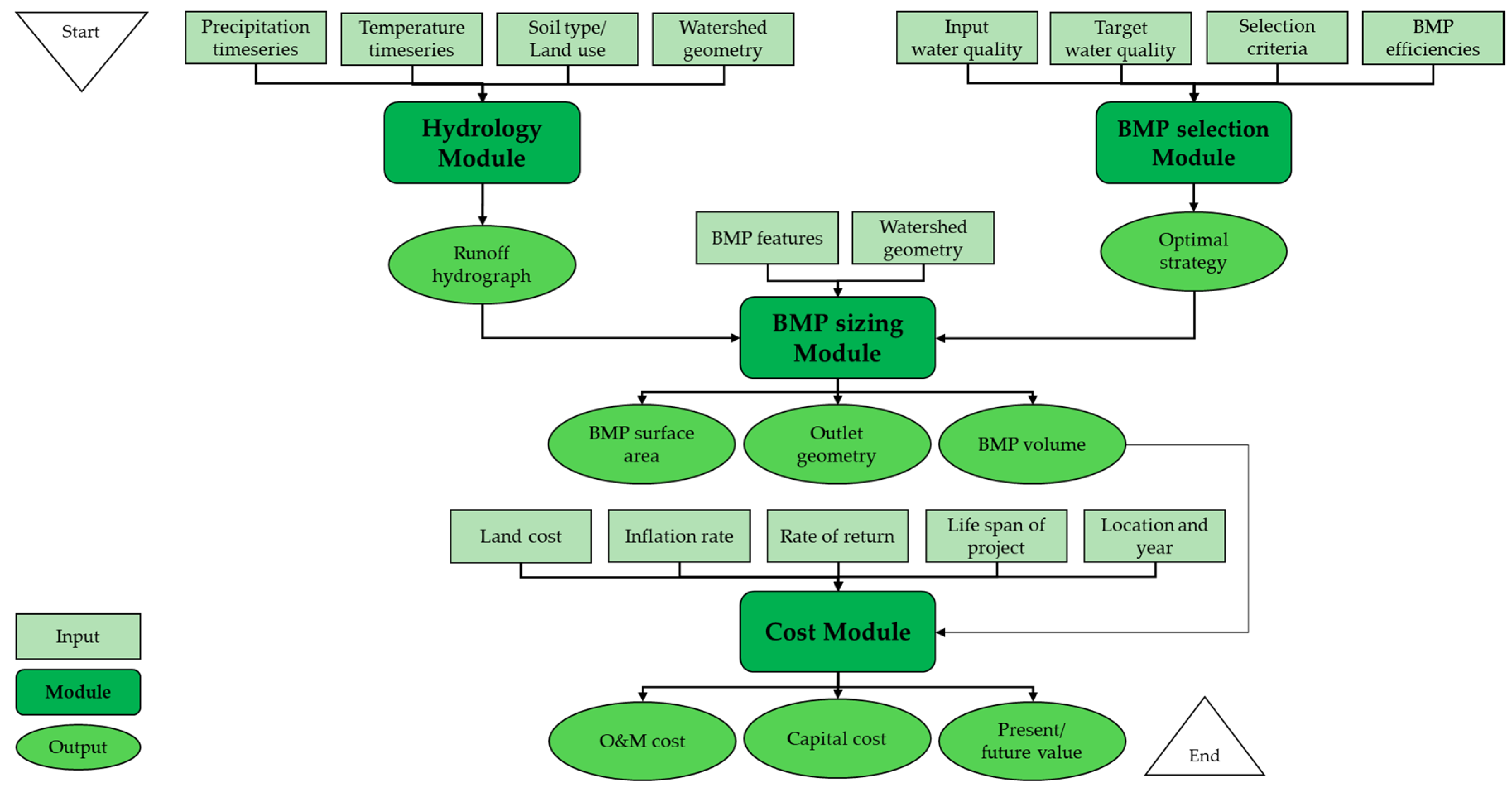
The section includes flowchart of the processes involved in i-DSTss and demonstration of the operation of the tool from the beginning to the end. Figure A1 demonstrates the modeling process included in the i-DSTss.
Figure A1. Flowchart describing i-DSTss.
Water 11 02022 g0a1
Demonstration of the operation of the tool are presented below. The first page of the tool is shown in Figure A2. Users can press the “Start the i-DST” button to go to the next page.
Figure A2. i-DSTss Introductory page.
Water 11 02022 g0a2
The interface in Figure A3 shows all the component modules in i-DSTss including hydrology module, BMP selection module, BMP sizing module, and the cost module.
Figure A3. i-DSTss Graphical User Interface (GUI).
Water 11 02022 g0a3
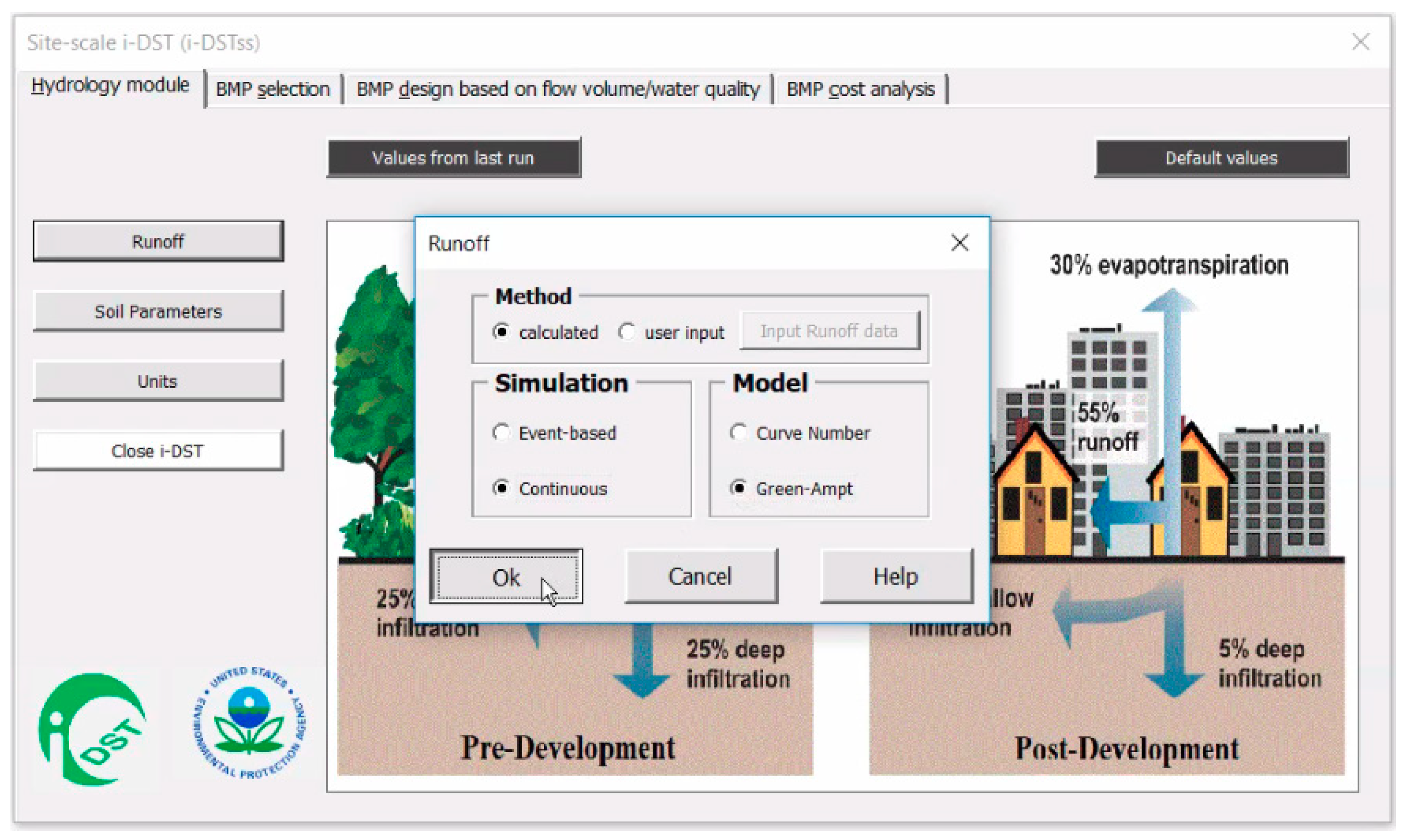
The hydrology module: The first module is the hydrology module. User can use hydrology module provided in i-DSTss or they may use outputs from another hydrology models. In the interface shown in Figure A4, users can select “user input” option to use their runoff data. Otherwise, they need to select the “calculated” option. As shown in Figure A4, event-based and continuous simulation options are provided. In both cases, users can select Green-Ampt or curve number method.
Figure A4. Hydrologic model Selection.
Water 11 02022 g0a4
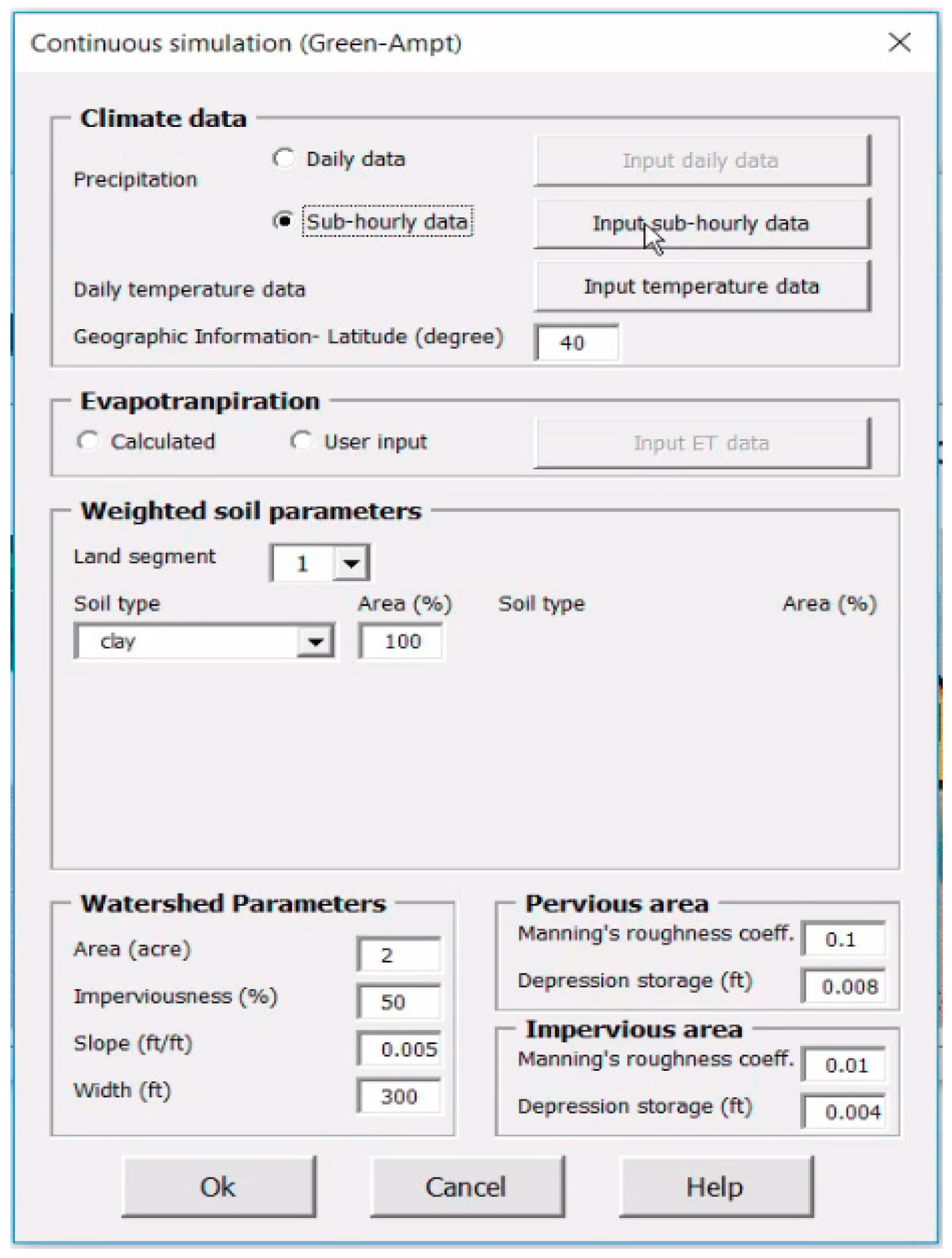
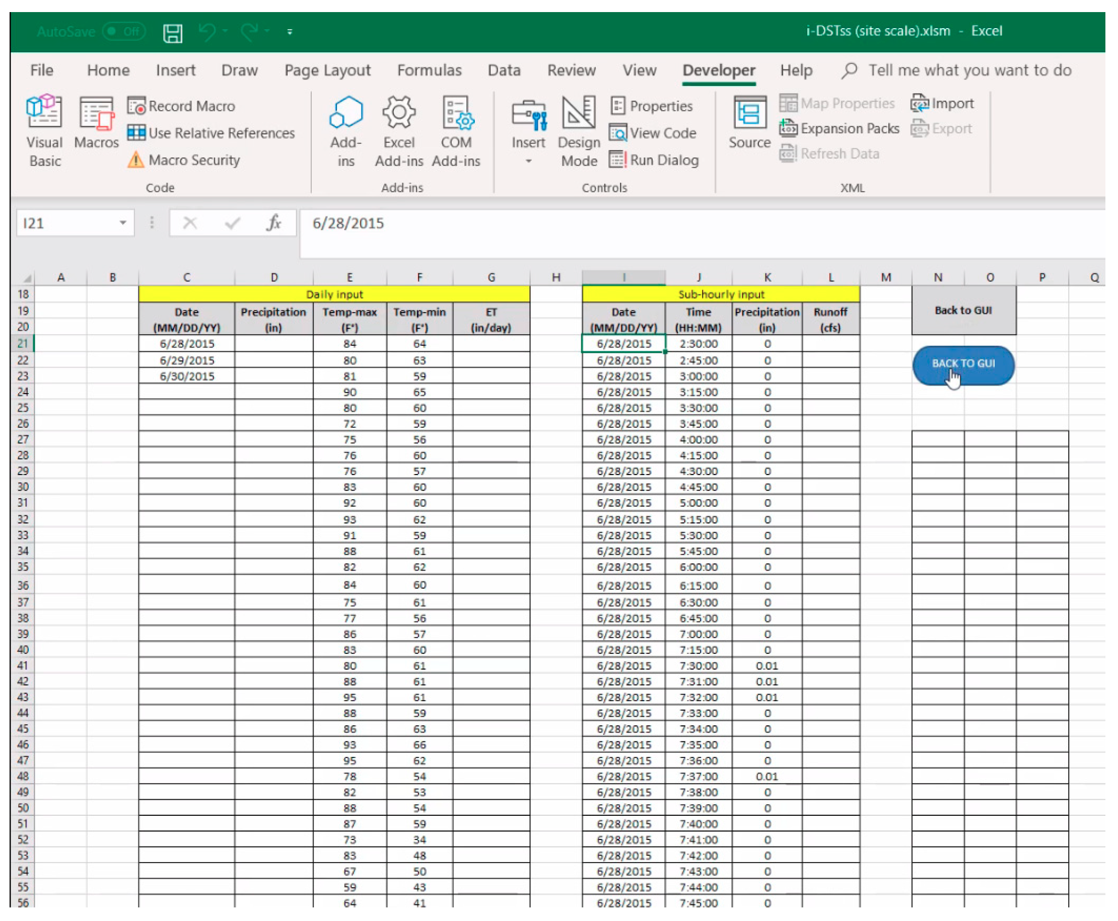
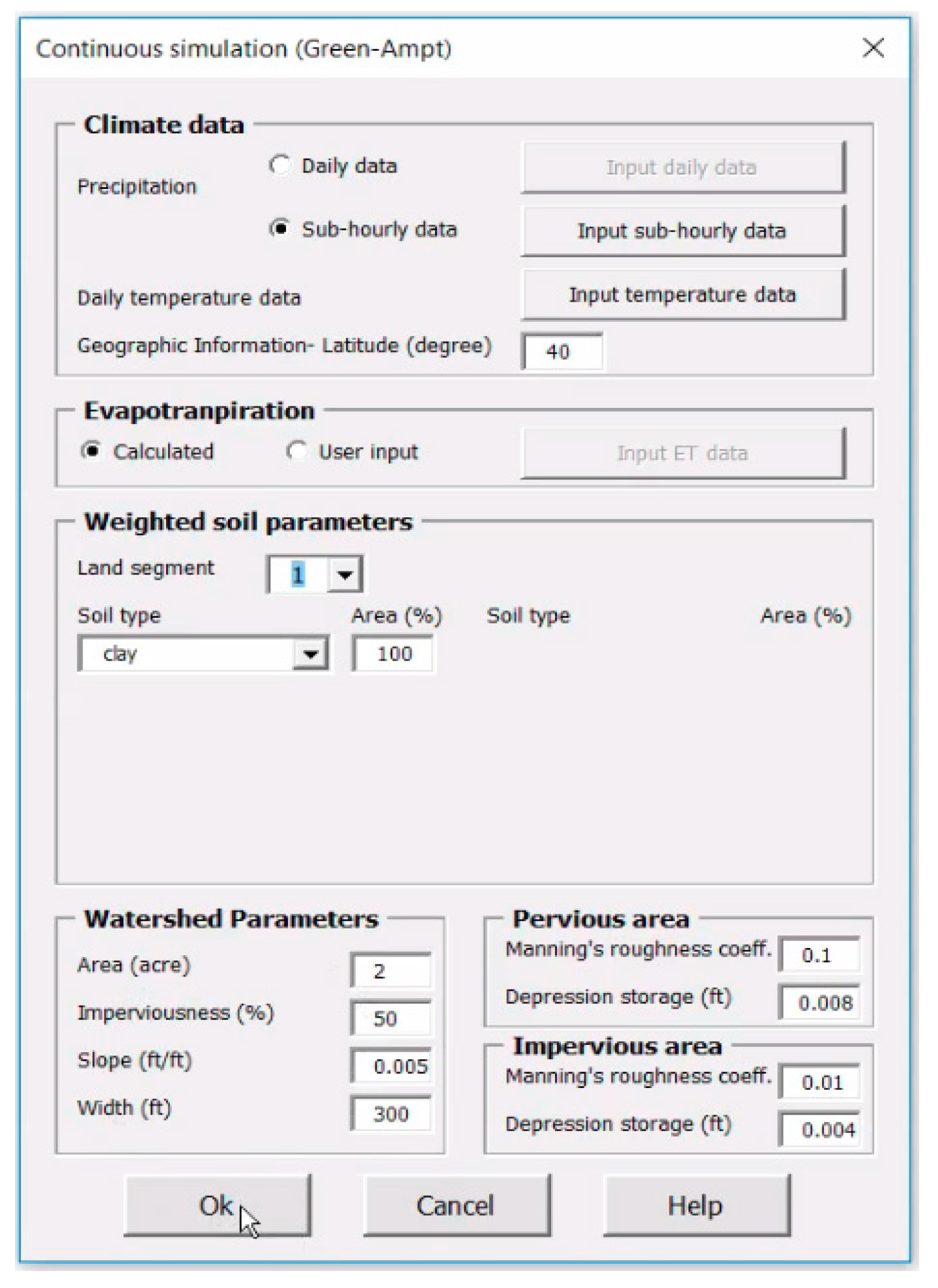
“Climate data”, “Evapotranspiration”, “Weighted soil parameters”, and “Watershed parameters” can be changed using the interface shown in Figure A5. For precipitation, the user may choose the daily or sub-hourly data to input the precipitation time series.
Figure A5. Input parameters for Green-Ampt model.
Water 11 02022 g0a5
If users select a sub-hourly data, they can input the precipitation time series data in the Excel spreadsheets which is linked to interface shown in Figure A5. After inputting the precipitation time series in the spreadsheet, the user can click “BACK TO GUI” button to come back to the Graphical User Interface (GUI) (Figure A6).
Figure A6. Precipitation time series input page.
Water 11 02022 g0a6
The “Weighted soil parameter” section allows inputting soils data for up to 10 land segments. Users can choose different soil types and percentage of area under each soil type. When users select a soil type, the soil parameters will be populated automatically (Figure A7).
Figure A7. Defining soil type and watershed parameters.
Water 11 02022 g0a7
The output pages in Figure A8 and Figure A9 show time series of runoff hydrograph, precipitation, and infiltration rate.
Figure A8. Displaying runoff hydrograph.
Water 11 02022 g0a8
Figure A9. Displaying infiltration rate.
Water 11 02022 g0a9
The BMP selection module: The BMP selection module selects a BMP type based on inflow water quality, target water quality, BMP removal efficiency and other criteria such as cost. The BMP selection module includes water quality data, BMP removal efficiency, user preference, and weighting inputs as shown in Figure A10.
Figure A10. BMP selection module.
Water 11 02022 g0a10
The water quality data is obtained from the national stormwater quality database. If the users have their own water quality data there is an option to input their own data (“Input data” button). The input water quality data changes with NCDC climates region, land use, and level of concentration. For the purpose of demonstration, the “Southeast” climate region, “Industrial” for land use, and “Median” concentration levels are selected (Figure A11).
Figure A11. Defining water quality inputs.
Water 11 02022 g0a11
The “Show water quality parameters” button can be used to display water quality data corresponding to climate region, land use, and concentration level. The BMP removal efficiencies for different BMP types are obtained from BMP international database. There is a “User preference” option which provides a list of BMPs. User can include or exclude BMPs from the selection process by selecting BMPs from Figure A12. The left side is for including BMPs and the right side is for excluding the BMPs.
Figure A12. List of BMPs to include or exclude.
Water 11 02022 g0a12
Also, in the “User weighting” input page shown in Figure A13, the user can input weights and scores for the different criteria used in the BMP selection process ranging from 0 to 5.
Figure A13. User weighting option.
Water 11 02022 g0a13
User can run the BMP selection module by clicking on “Run BMP Selection” button. The optimal BMP will be selected using an optimization procedure. For instance, here a wetland has been selected. Once the data is input, users can run the model to select a BMP type. The select BMP type will be displayed in the box shown in Figure A14 under the “Run BMP selection” button.
Figure A14. Output of BMP selection module.
Water 11 02022 g0a14
The BMP sizing module: For the purpose of sizing, BMPs have been categorized into three different groups including green roof system, infiltration based BMPs such as bioretention and storage-based BMPs such as detention and retention pond (Figure A15).
Figure A15. BMP sizing module.
Water 11 02022 g0a15
(a)
Green roof system: In the “Green roof system”, the goal is to determine how much area has to be under the green roof to achieve a specific percent flow reduction. The area of the watershed, percent imperviousness and the runoff hydrograph come from the hydrology module. As shown in Figure A16, by running the tool for 20 percent flow reduction, the surface area that has to be under a green roof is calculated. User may also view the hydrographs from the graphical output. In the Figure A16 the blue line shows the hydrograph without green roof and the red line shows the hydrograph with green roof.
Figure A16. Output hydrograph for green roof system.
Water 11 02022 g0a16
(b)
Infiltration-based BMPs: The next group of BMPs are infiltration-based BMPs. For the infiltration-based BMPs, the user inputs the area of the BMP and the tool will calculate the percent capture and drawdown time. The tool also shows the graphical outputs of inflow and outflow hydrographs as shown in Figure A17.
Figure A17. Output hydrograph for infiltration-based BMPs.
Water 11 02022 g0a17
The tool also tracks the water level inside the surface (ponding) layer (Figure A18).
Figure A18. Water level tracking in infiltration-based BMPs.
Water 11 02022 g0a18
(c)
Storage-based BMPs: The third group of BMPs are storage-based BMPs such as detention pond and retention pond. Since ponds usually are used for stormwater management for bigger area, the area of watershed has been increased in this scenario. The input is percent peak flow reduction and the output is geometry of the pond and geometry of the outlet structures. By inputting 50 percent peak flow reduction and other input parameters, the tool determines optimal size/geometries of pond and outlet structures through an optimization process. By minimizing the size/volume of the pond, the cost will be minimized. Users can view inflow and outflow hydrographs and the peak flow reduction in the graphical output section as shown in Figure A19.
Figure A19. Output hydrograph for storage-based BMPs.
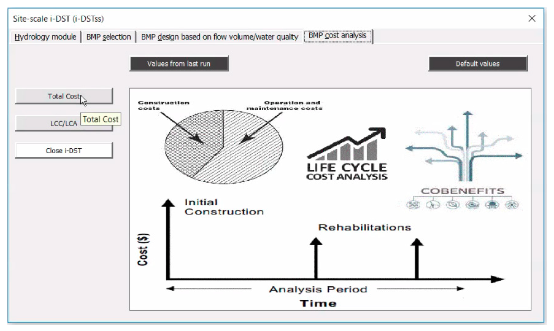
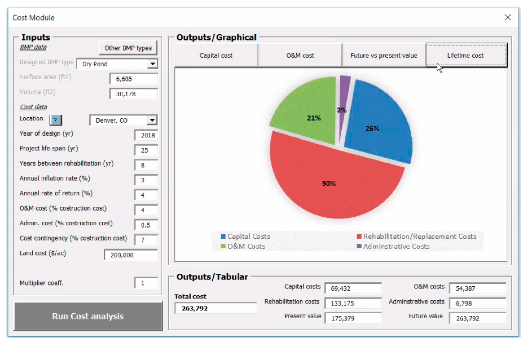
Water 11 02022 g0a19
The cost module: The last module is BMP cost module (Figure A20). The cost estimate is based on the size of the BMP determined using the BMP sizing module above. The size information from sizing module will be transferred to the cost module. For example, dry pond was used in the BMP sizing module, the data from BMP sizing module (surface area and the volume) are displayed here automatically.
Figure A20. Cost Module.
Water 11 02022 g0a20
User can also use the cost module to calculate cost of other BMP types by clicking on “Other BMP type” button and selecting a BMP type and input the area and volume to calculate the cost.
ENR cost data for the 20 cities in the United States have been used and user can change the different cities. If a city is not listed, they can use the Thiessen polygon and use the data from the closest city
After running the cost analysis, the total cost will be calculated. The total cost includes capital cost, operation maintenance costs and other related costs. The tool displays graphical outputs of capital costs, rehabilitation cost, operation maintenance costs, administration costs, and present value. The tool will also show the distribution of all components of cost over the lifetime of the project as shown in Figure A21.
Figure A21. Distribution of cost components over the lifetime of the project.
Water 11 02022 g0a21

References

  1. Tetra Tech. User’s Guide Spreadsheet Tool for the Estimation of Pollutant Load (STEPL); Tetra Tech, Inc.: Fairfax, VA, USA, 2011. [Google Scholar]
  2. Grimm, N.B.; Faeth, S.H.; Golubiewski, N.E.; Redman, C.L.; Wu, J.; Bai, X.; Briggs, J.M. Global change and the ecology of cities. Science 2008, 319, 756–760. [Google Scholar] [CrossRef] [PubMed]
  3. Dietz, M.E. Low impact development practices: A review of current research and recommendations for future directions. Water Air Soil Pollut. 2007, 186, 351–363. [Google Scholar] [CrossRef]
  4. Brabec, E.; Schulte, S.; Richards, P.L. Impervious surfaces and water quality: A review of current literature and its implications for watershed planning. J. Plan. Lit. 2002, 16, 499–514. [Google Scholar] [CrossRef]
  5. Montgomery, M. United Nations Population Fund: State of world population 2007: Unleashing the potential of urban growth. Popul. Dev. Rev. 2007, 33, 639–641. [Google Scholar]
  6. Parkinson, J. Drainage and stormwater management strategies for low-income urban communities. Environ. Urban. 2003, 15, 115–126. [Google Scholar] [CrossRef] [Green Version]
  7. Fletcher, T.D.; Shuster, W.; Hunt, W.F.; Ashley, R.; Butler, D.; Arthur, S.; Trowsdale, S.; Barraud, S.; Semadeni-Davies, A.; Bertrand-Krajewski, J.L. SUDS, LID, BMPs, WSUD and more–The evolution and application of terminology surrounding urban drainage. Urban Water J. 2015, 12, 525–542. [Google Scholar] [CrossRef]
  8. Medina, F.M.; Bonnaud, E.; Vidal, E.; Tershy, B.R.; Zavaleta, E.S.; Donlan, C.J.; Keitt, B.S.; le Corre, M.; Horwath, S.V.; Nogales, M. A global review of the impacts of invasive cats on island endangered vertebrates. Glob. Chang. Biol. 2011, 17, 3503–3510. [Google Scholar] [CrossRef]
  9. Coffman, L.; Cheng, M.S.; Weinstein, N.; Clar, M. Low-Impact Development Hydrologic Analysis and Design. In Water Resources and the Urban Environment; ASCE: New York, NY, USA, 1998. [Google Scholar]
  10. Dietz, M.E.; Clausen, J.C. Stormwater runoff and export changes with development in a traditional and low impact subdivision. J. Environ. Manag. 2008, 87, 560–566. [Google Scholar] [CrossRef]
  11. Khader, O.; Montalto, F.A. Development and Calibration of a High Resolution SWMM Model for Simulating the Effects of LID Retrofits on the Outflow Hydrograph of a Dense Urban Watershed. In Low Impact Development for Urban Ecosystem and Habitat Protection; American Society of Civil Engineers: Reston, VA, USA, 2009. [Google Scholar] [CrossRef]
  12. US Environmental Protection Agency (EPA). Low Impact Development (LID): A Literature Review; US Environmental Protection Agency Office of Water: Washington, DC, USA, 2000. [Google Scholar]
  13. Montalto, F.; Behr, C.; Alfredo, K.; Wolf, M.; Arye, M.; Walsh, M. Rapid assessment of the cost-effectiveness of low impact development for CSO control. Landsc. Urban Plan. 2007, 82, 117–131. [Google Scholar] [CrossRef]
  14. Tu, M.C. A New Method to Assess. Best Management Practice Efficiency to Optimize Storm Water Management. Ph.D. Thesis, Texas A & M University, College Station, TX, USA, 2014. Available online: http://hdl.handle.net/1969.1/153810 (accessed on 16 December 2014).
  15. Connor, T.O.; Sullivan, D.; Clar, M.; Barfield, B. Considerations in the design of treatment best management practices (BMPs) to improve water quality. Proc. Water Environ. Fed. 2003, 2003, 1186–1205. [Google Scholar] [CrossRef]
  16. Fraley-McNeal, L.; Schueler, T.; Winer, R. National Pollutant Removal Performance Database, Version 3; Center for Watershed Protection: Ellicott City, MD, USA, 2007; pp. 1–10. [Google Scholar]
  17. Ellis, J. Infiltration systems: A sustainable source—control option for urban stormwater quality management? Water Environ. J. 2000, 14, 27–34. [Google Scholar] [CrossRef]
  18. Reynolds, S.K.; Pomeroy, C.A.; Rowney, A.C.; Rowney, C.M. Linking Stormwater BMP Systems Water Quality and Quantity Performance to Whole Life Cycle Cost to Improve BMP Selection and Design. In World Environmental and Water Resources Congress 2012: Crossing Boundaries, Albuquerque, NM, USA, 20–24 May 2012; Loucks, E.D., Ed.; American Society of Civil Engineers: Reston, VA, USA, 2012. [Google Scholar]
  19. Guo, Q.; Correa, C.A. The Impacts of Green Infrastructure on Flood Level Reduction for the Raritan River: Modeling Assessment. In World Environmental and Water Resources Congress 2013: Showcasing the Future, Cincinnati, OH, USA, 19–23 May 2013; Patterson, C.L., Struck, S.D., Murray, D.J., Jr., Eds.; American Society of Civil Engineers: Reston, VA, USA, 2013. [Google Scholar]
  20. James, W.; Rossman, L.A.; James, W.R.C. User’s Guide to SWMM 5; CHI: Guelph, ON, Canada, 2010. [Google Scholar]
  21. Pitt, R.; Voorhees, J. SLAMM, the source loading and management model. In Wet-Weather Flow in the Urban Watershed: Technology and Management; CRC Press: Boca raton, FL, USA, 2002; pp. 103–139. [Google Scholar]
  22. Lai, F.H.; Zhen, J.; Riverson, J.; Alvi, K.; Shoemaker, L. Multiple Watershed Scales Approach for Placement of Best Management Practices in SUSTAIN. In World Environmental and Water Resources Congress 2009: Great Rivers; Kansas City, MO, USA, 17–21 May 2009; Starrett, S., Ed.; American Society of Civil Engineers: Reston, VA, USA, 2009. [Google Scholar]
  23. Tang, Z.; Engel, B.; Pijanowski, B.; Lim, K. Forecasting land use change and its environmental impact at a watershed scale. J. Environ. Manag. 2005, 76, 35–45. [Google Scholar] [CrossRef] [PubMed]
  24. Wong, T.H.; Fletcher, T.D.; Duncan, H.P.; Jenkins, G.A. Modelling urban stormwater treatment—A unified approach. Ecol. Eng. 2006, 27, 58–70. [Google Scholar] [CrossRef]
  25. Rossman, L.A.; Bernagros, J.T. National Stormwater Calculator User’s Guide–Version 1.2. 0.1; EPA: Washington, DC, USA, 2014. [Google Scholar]
  26. Minnesota Stormwater Manual, Overview of Minimal Impact Design Standards (MIDS); Minnesota Pollution Control Agency: Rochester, MN, USA, 2016.
  27. California State University (Sacramento). California Phase II LID Sizing Tool Documentation Manual; California State University: Sacramento, CA, USA, 2019. [Google Scholar]
  28. Johnson, R.; Sample, D. A semi-distributed model for locating stormwater best management practices in coastal environments. Environ. Model. Softw. 2017, 91, 70–86. [Google Scholar] [CrossRef] [Green Version]
  29. Alamdari, N.; Sample, D.J. A multiobjective simulation-optimization tool for assisting in urban watershed restoration planning. J. Clean. Prod. 2019, 213, 251–261. [Google Scholar] [CrossRef]
  30. King, K.W.; Arnold, J.; Bingner, R. Comparison of Green-Ampt and curve number methods on Goodwin Creek watershed using SWAT. Trans. ASAE 1999, 42, 919. [Google Scholar] [CrossRef]
  31. Doherty, J.; Christensen, S. Use of paired simple and complex models to reduce predictive bias and quantify uncertainty. Water Resour. Res. 2011, 47. [Google Scholar] [CrossRef] [Green Version]
  32. Green, W.H.; Ampt, G. Studies on Soil Phyics. J. Agric. Sci. 1911, 4, 1–24. [Google Scholar]
  33. Boughton, W. A review of the USDA SCS curve number method. Soil Res. 1989, 27, 511–523. [Google Scholar] [CrossRef]
  34. Hargreaves, G.H.; Samani, Z.A. Reference crop evapotranspiration from temperature. Appl. Eng. Agric. 1985, 1, 96–99. [Google Scholar] [CrossRef]
  35. Fleming, P. A diurnal distribution function for daily evaporation. Water Resour. Res. 1970, 6, 937–942. [Google Scholar] [CrossRef]
  36. Liu, S.; Graham, W.D.; Jacobs, J.M. Daily potential evapotranspiration and diurnal climate forcings: Influence on the numerical modelling of soil water dynamics and evapotranspiration. J. Hydrol. 2005, 309, 39–52. [Google Scholar] [CrossRef]
  37. Barry, D.; Parlange, J.Y.; Li, L.; Jeng, D.S.; Crapper, M. Green–Ampt approximations. Adv. Water Resour. 2005, 28, 1003–1009. [Google Scholar] [CrossRef]
  38. Ali, S.; Islam, A.; Mishra, P.; Sikka, A.K. Green-Ampt approximations: A comprehensive analysis. J. Hydrol. 2016, 535, 340–355. [Google Scholar] [CrossRef]
  39. Mizumura, K. Analytical Solutions of Nonlinear Kinematic Wave Model. J. Hydrol. Eng. 2006, 11, 539–546. [Google Scholar] [CrossRef]
  40. Pitt, R.; Maestre, A.; Clary, J. The National Stormwater Quality Database (NSQD, Version 4.02); Department of Civil and Environmental Engineering; University of Alabama: Tuscaloosa, AL, USA, 2018. [Google Scholar]
  41. International Stormwater BMP Database. Developed by Wright Water Engineers, Inc. and Geosyntec Consultants for the Water Research Foundation (WRF), the American Society of Civil Engineers (ASCE)/Environmental and Water Resources Institute (EWRI), the American Public Works Association (APWA), the Federal Highway Administration (FHWA), and U.S. Environmental Protection Agency (EPA). 2018. Available online: http://www.bmpdatabase.org/download-master.html (accessed on 22 August 2018).
  42. Ma, G.; Geza, M.; Cath, T.Y.; Drewes, J.E.; Xu, P. iDST: An. integrated decision support tool for treatment and beneficial use of non-traditional water supplies–Part. II. Marcellus and Barnett Shale case studies. J. Water Process Eng. 2018, 25, 258–268. [Google Scholar] [CrossRef]
  43. Ravindran, A.R.; Warsing, D.P., Jr. Supply Chain Engineering: Models and Applications; CRC Press: Boca Raton, FL, USA, 2016. [Google Scholar]
  44. Kasprzak, E.M.; Lewis, K.E. Pareto analysis in multiobjective optimization using the collinearity theorem and scaling method. Struct. Multi. Optim. 2001, 22, 208–218. [Google Scholar] [CrossRef]
  45. Feddes, R.; Zaradny, H. Model for simulating soil-water content considering evapotranspiration—Comments. J. Hydrol. 1978, 37, 393–397. [Google Scholar] [CrossRef]
  46. Chow, V.T.; Maidment, D.R.; Mays, L.W. Applied Hydrology; McGraw Hill: New York, NY, USA, 1988. [Google Scholar]
  47. Sample, D.J.; Heaney, J.P.; Wright, L.T.; Fan, C.Y.; Lai, F.H.; Field, R. Costs of best management practices and associated land for urban stormwater control. J. Water Resour. Plan. Manag. 2003, 129, 59–68. [Google Scholar] [CrossRef]
  48. Heaney, J.P.; Sample, D.; Wright, L. Costs of Urban Stormwater Control; US Environmental Protection Agency, Office of Research and Development: Washington, DC, USA, 2002.
  49. California Stormwater Quality Association. California Stormwater BMP Handbook–New Development and Redevelopment; California Stormwater Quality Association: Menlo Park, CA, USA, 2003. [Google Scholar]
  50. Narayanan, A.; Pitt, R. Costs of Urban Stormwater Control Practices; Citeseer: Forest Grove, OR, USA, 2006. [Google Scholar]
  51. Selbig, W.R. Evaluation of leaf removal as a means to reduce nutrient concentrations and loads in urban stormwater. Sci. Total Environ. 2016, 571, 124–133. [Google Scholar] [CrossRef]
  52. Anand, S.; Mankin, K.R.; McVay, K.A.; Janssen, K.A.; Barnes, P.L.; Pierzynski, G.M. Calibration and Validation of ADAPT and SWAT for Field—Scale Runoff Prediction 1. J. Am. Water Resour. Assoc. 2007, 43, 899–910. [Google Scholar] [CrossRef]
  53. White, K.L.; Chaubey, I. Sensitivity analysis, calibration, and validations for a multisite and multivariable SWAT model 1. J. Am. Water Resour. Assoc. 2005, 41, 1077–1089. [Google Scholar] [CrossRef]
  54. Santhi, C.; Arnold, J.G.; Williams, J.R.; Dugas, W.A.; Srinivasan, R.; Hauck, L.M. Validation of the swat model on a large rwer basin with point and nonpoint sources 1. J. Am. Water Resour. Assoc. 2001, 37, 1169–1188. [Google Scholar] [CrossRef]
  55. Legates, D.R.; McCabe, G.J., Jr. Evaluating the use of “goodness-of-fit” measures in hydrologic and hydroclimatic model validation. Water Resour. Res. 1999, 35, 233–241. [Google Scholar] [CrossRef]
  56. Nash, J.E.; Sutcliffe, J.V. River flow forecasting through conceptual models part I—A discussion of principles. J. Hydrol. 1970, 10, 282–290. [Google Scholar] [CrossRef]
  57. Chu, T.; Shirmohammadi, A. Evaluation of the SWAT model’s hydrology component in the piedmont physiographic region of Maryland. Trans. ASAE 2004, 47, 1057. [Google Scholar] [CrossRef]
  58. Geza, M.; Poeter, E.P.; McCray, J.E. Quantifying predictive uncertainty for a mountain-watershed model. J. Hydrol. 2009, 376, 170–181. [Google Scholar] [CrossRef]
  59. Moriasi, D.N.; Gitau, M.W.; Pai, N.; Daggupati, P. Hydrologic and water quality models: Performance measures and evaluation criteria. Trans. ASABE 2015, 58, 1763–1785. [Google Scholar]
  60. Selbig, W.R.; Buer, N. Hydraulic, Water-Quality, and Temperature Performance of Three Types of Permeable Pavement under High Sediment Loading Conditions; US Geological Survey: Menlo Park, CA, USA, 2018.
  61. Druzdzel, M.J.; Flynn, R.R. Decision Support Systems. Encyclopedia of Library and Information Science. A. Kent; Marcel Dekker, Inc.: New York, NY, USA, 1999; Volume 10, p. 2010. [Google Scholar]
  62. Flores, X.; Rodríguez-Roda, I.; Poch, M.; Jiménez, L.; Bañares-Alcántara, R. Systematic procedure to handle critical decisions during the conceptual design of activated sludge plants. Ind. Eng. Chem. Res. 2007, 46, 5600–5613. [Google Scholar] [CrossRef]
  63. Rodriguez-Roda, I.; Poch, M.; Bañares-Alcántara, R. Conceptual design of wastewater treatment plants using a design support system. J. Chem. Technol. Biotechnol.: Int. Res. Process Environ. Clean Technol. 2000, 75, 73–81. [Google Scholar] [CrossRef]
  64. Gachet, A.; Sprague, R. A Context-Based Approach to the Development of Decision Support Systems. International Workshop on Context Modeling and Decision Support; Paris, France, 2015. Available online: http://citeseerx.ist.psu.edu/viewdoc/similar?doi=10.1.1.143.1230&type=ab (accessed on 28 September 2019).
  65. Freitas, I.S.; Costa, C.A.; Boaventura, R.A. Conceptual design of industrial wastewater treatment processes: Primary treatment. Comput. Chem. Eng. 2000, 24, 1725–1730. [Google Scholar] [CrossRef]
  66. Geza, M.; Ma, G.; Kim, H.; Cath, T.Y.; Xu, P. iDST: An. integrated decision support tool for treatment and beneficial use of non-traditional water supplies–Part. I. Methodology. J. Water Process Eng. 2018, 25, 236–246. [Google Scholar] [CrossRef]
Figure 1. Conceptual framework for the hydrology module.
Water 11 02022 g001
Figure 2. Conceptual framework of BMP selection module.
Water 11 02022 g002
Figure 3. BMP selection criteria.
Water 11 02022 g003
Figure 4. Input water quality data based on NCDC climate region, land use.
Water 11 02022 g004
Figure 5. Schematic pattern of mass balance for infiltration-based BMPs in three separate layers.
Water 11 02022 g005
Figure 6. Conceptual framework of optimization approach for storage-based BMP.
Water 11 02022 g006
Figure 7. Distributed capital, rehabilitation and O&M costs over 25 years lifetime of project.
Water 11 02022 g007
Figure 8. Effective percentage of each cost component over 25 years lifetime of project.
Water 11 02022 g008
Figure 9. Yellowstone Drive catchment (WI) plan.
Water 11 02022 g009
Figure 10. (a) Comparison of observed and simulated runoff for Yellowstone Drive catchment (b) Scatter diagram of observed and simulated data.
Water 11 02022 g010
Figure 11. (a) Comparison of observed and simulated runoff for a small parking lot (b) Scatter diagram of observed and simulated data.
Water 11 02022 g011aWater 11 02022 g011b
Figure 12. Default weights for different criteria in BMP selection module.
Water 11 02022 g012
Figure 13. Observed versus modeled outflow hydrograph.
Water 11 02022 g013
Figure 14. Comparison of green roof modelling with observed data.
Water 11 02022 g014
Figure 15. Parking lot located in Madison, Wisconsin.
Water 11 02022 g015
Figure 16. Measures versus simulated outflow volume.
Water 11 02022 g016
Figure 17. Comparison of simulated outflow versus observed outflow.
Water 11 02022 g017
Figure 18. Inflow and outflow hydrograph for (a) 25 percent peak flow reduction and (b) 50 percent peak flow reduction.
Water 11 02022 g018
Figure 19. Graphical user interface (GUI) of i-DSTss (BMP sizing module).
Water 11 02022 g019
Table 1. Comparison of existing stormwater management tools.
ToolCapabilities/Features
Developing EnvironmentRunoff VolumePeak FlowPollutant Loads/Concentration 1BMP/GICost/LCCA 2Integrated Optimization 3Water Quality Analysis 4
WERF SELECT [18]Excel-VBA
Green Values [19] JavaScript
STEPL [1]Excel-VBA
EPA SWMM 5 [20]C language
WinSLAMM [21]Fortran
EPA SUSTAIN [22]C language
L-THIA [23]Excel-VBA
MUSIC [24]Fortran
LIDRA [13]Visual studio, C# language
Stormwater calculator [25]C language
MIDS calculator [26]Excel-VBA
California LID Sizing Tool [27]Visual basic, JavaScript
BMP Checker [28]Python
RSWMM-Cost [29]R language
i-DSTssExcel-VBA
1 Pollutant load/Concentration refers to the load or concentration of pollutants discharged into the outlet or into a BMP from the catchment/watershed; 2 LCCA is a cost estimation method for incorporating all phases of project’s life useful in selecting between mutually exclusive options; 3 Integrated optimization refers to an optimization approach where multiple criteria including environmental, social, technical and economic factors are used in the optimization process; 4 Water quality analysis refers to BMP treatment performance evaluation.
Table 2. BMP selection sustainability criteria (user weighting component).
CategoryCriteriaDescription
EconomicLCALife cycle cost of a BMP
Capital, O&M costsCost of installation, operation and maintenance for a BMP
Property valueLand cost and related property value of a BMP
EnvironmentalFlow reductionPotential for runoff volume captured or peak flow reduction
Pollutant reductionPollutant load reduction potential
Green spacePotential for creating green space covered with grass or trees
SocialAestheticsPotential for creation of scenic values
Community AcceptanceAcceptance by the community, affected populations including local stakeholders and authorities
NuisancesCreating inconvenience or annoyances
TechnicalMaterial availability Relative ease of obtaining construction materials
FeasibilityLikelihood that projects can be easily implemented
Ease of Maintenance and operationRelative ease of operation and maintenance if failure occurs due to clogging or other factors
Table 3. Cost categories during the life cycle of the project.
Cost CategoryDescription
Capital costsConstruction costBMP construction cost
Land cost (user input value)Cost of acquiring the land
Cost contingency, % of construction cost (~7%)Unexpected cost
O&M costs, % of construction cost (~4%)Costs incurred each year for maintenance and operation
Rehabilitation costs, % of construction cost (~70%)Cost for replacing a BMP
Administrative and inspection costs, % of construction cost (~0.5%)Inspection cost
Table 4. Percentage of area under each land cover.
Land Cover TypePercent Area
Streets17%
Driveways6%
Roofs17%
Sidewalks5%
Other Impervious<1%
Lawns/Open55%
Table 5. BMP selection by land use (residential) and pollutant concentration.
Land UseWater Quality Parameter (unit)Level of Concentration
MinMedianMax
ResidentialTSS (mgL)0.2538.002380.52
TP (mgL)0.010.2321.20
TN (mgL)0.201.5110.30
Bacteria (100 mL)25.501870.0048,392.00
Pb (ugL)0.155.00368.00
Zn (ugL)1.0074.002077.40
Cu (mgL)0.5010.007270.00
NO3 (mgL)0.050.641.26
PO4 (mgL)0.000.106.00
Optimal BMPRain gardenBioretentionVFS-Bioretention
Table 6. BMP selection by land use (industrial) and pollutant concentration.
Land UseWater Quality Parameter (unit)Level of Concentration
MinMedianMax
IndustrialTSS (mgL)0.5048.001130.00
TP (mgL)0.010.192.14
TN (mgL)0.212.038.01
Bacteria (100 mL)25.501870.0048,392.00
Pb (ugL)0.106.80370.00
Zn (ugL)1.00101.007700.00
Cu (mgL)1.0010.00950.00
NO3 (mgL)0.130.511.24
PO4 (mgL)0.000.106.00
Optimal BMPWetlandWetlandForebay-Wetland
Table 7. BMP selection by land use (freeways) and pollutant concentration.
Land UseWater Quality Parameter (unit)Level of Concentration
MinMedianMax
FreewaysTSS (mgL)0.5033.00823.00
TP (mgL)0.010.253.35
TN (mgL)0.200.848.14
Bacteria (100 mL)25.501870.0048,392.00
Pb (ugL)0.155.20230.00
Zn (ugL)1.0048.001000.00
Cu (mgL)1.006.00122.00
NO3 (mgL)0.030.512.20
PO4 (mgL)0.000.106.00
Optimal BMPGrass swaleGrass swaleForebay-Grass swale
Table 8. Summary for two different scenarios (50 and 25 percent peak flow reduction).
Peak Flow Reduction (%)5025
Pond depth (m)1.81.3
Pond storage (m3)17064
Pond surface area (m2)9549
Length at bottom (m)6.14.2
Width at bottom (m)2.01.4
Total discharge by weir and orifice (cms)2.732.57