Article

Impacts of Climate Change Scenarios on Non-Point Source Pollution in the Saemangeum Watershed, South Korea

School of Architectural, Civil, Environmental, and Energy Engineering, Kyungpook National University, 80 Daehak-ro, Buk-gu, Daegu 41566, Korea
*
Author to whom correspondence should be addressed.
Water 2019, 11(10), 1982; https://doi.org/10.3390/w11101982
Submission received: 23 July 2019 / Revised: 3 September 2019 / Accepted: 21 September 2019 / Published: 23 September 2019
(This article belongs to the Section Water Resources Management, Policy and Governance)

Abstract

:
Non-point source (NPS) pollution is a primary cause of water pollution in the Saemangeum watershed in South Korea. The changes in NPS pollutant loads in the Saemangeum watershed for an 81-year period (2019–2099) were simulated and analyzed by applying the soil and water assessment tool. Six climate model (BCC-CSM1–1, CanESM2, GFDL-ESM2G, HadGEM2-CC, INM-CM4, and MIROC-ESM) outputs using representative concentration pathway (RCP) scenarios (RCP 4.5 and RCP 8.5) were obtained from the South Korean Asia-Pacific Economic Cooperation (APEC) Climate Center. Simulated streamflow and water quality were evaluated using the Nash–Sutcliffe efficiency (NSE) index and coefficient of determination (R2). The model satisfactorily simulated streamflow with positive NSE values and R2 > 0.5. Based on two climate change scenarios (RCP 4.5 and RCP 8.5), gradual increases of 70.9 to 233.8 mm and 1.7 to 5.7 °C in annual precipitation and temperature, respectively, are likely for two time periods (2019–2059 and 2060–2099). Additionally, the expected future average annual and monthly streamflow, sediment, and total phosphorus showed changes of 5% to 43%, 3% to 40%, and −55% to 15%, respectively, whereas the expected future average annual and monthly total nitrogen showed decreases of −5% to −27%. Future NPS pollutant loads in the Saemangeum watershed should be managed according to different climate change scenarios.

1. Introduction

Climate change is a key global environmental concern due to regional rainfall and temperature changes affecting regional hydrological cycles, which impact streamflow discharge, water quality, human health, and the environment [1,2]. For example, the Korea Meteorological Administration has estimated that the mean atmospheric temperature and precipitation in South Korea are likely to increase by 5.7 °C and 17.6%, respectively, by the end of the 21st century based on the most severe greenhouse gas emissions scenarios [1]. Therefore, water resources planning and water quality management should consider the impacts of these potential climate changes [3]. Surface water in particular is influenced by rainfall or human activities and is widely recognized as a receptor of refuse and agricultural pollution [3]. Therefore, surface water quality monitoring is an important step toward the effective management of water resources and requires certain maintenance at or above a certain level depending on the usage [4]. Surface water pollution sources can generally be classified as point source or non-point source (NPS) pollution. The latter has caused increasing concern due to its substantial contribution to the deterioration of the aquatic environment [5].
The South Korean Ministry of Environment has reported that NPS pollution is among the primary causes of water pollution in the Saemangeum watershed. The Saemangeum watershed plays an important role in the allocation of water resources in South Korea. The Saemangeum seawall is the world’s longest sea dike, and has a reclaimed land area of 283 km2 with a 118 km2 lake [6]. The major purpose of the Saemangeum project was to develop the reclaimed land and provide fresh water for agricultural development; serious concern was expressed about the potential environmental problems due to the project, such as water quality deterioration related to industrial and agricultural pollution [7]. However, evaluating NPS pollution from industrial and agricultural activities on a large scale, such as the Saemangeum project, requires process-based modeling [8]. Considerable research has been conducted on the management of the Saemangeum watershed. Oh et al. [9] predicted the desalination time of the Saemangeum reservoir using a numerical model. Woo et al. [8] investigated NPS pollution management in the Saemangeum watershed using the analytical hierarchy process technique. Kim et al. [10] investigated the causes of changes in water quality over time using statistical analysis. Monica and Choi [11] performed temporal and spatial analyses of water quality in the watershed using multivariate techniques. However, the simulation of water quality using the soil and water assessment tool (SWAT) has not been thoroughly explored for the analysis of large watersheds [12]. The abovementioned studies focused only on one of the two major sub-watersheds of the Saemangeum watershed. Therefore, we focused on the SWAT to accurately model and simulate runoff and water quality over a large area and evaluate the impacts of future climate change on runoff discharge and water quality.
SWAT is a physically based and spatially distributed hydrological model that is used for a wide range of purposes, such as simulation and evaluation of the impacts of land use and catchment management practices on water quality and quantity over various spatial and temporal scales [13]. The model has been proven to be effective for assessing water resources, especially in the simulation of hydrologic and water quality [3,14]. SWAT modeling has been used to assess the impacts of future climate change on NPS pollution [5]. Therefore, we aimed to assess the characteristics of future changes in NPS pollutant loads such as sediment, total nitrogen (TN) and total phosphorus (TP) in the Saemangeum watershed under the two representative concentration pathway (RCP) climate change scenarios (RCP 4.5 and RCP 8.5) for the next 81 years (2019–2099).

2. Materials and Methods

2.1. Study Area and Input Data

The Saemangeum watershed is located in Jeollabuk-do province, Southwestern South Korea (36°60′ N, 127°28′ E). It has a drainage area of 3300 km2, an average slope of 0.1°, and an elevation of 4–7 m [15]. The predominant soil type is loam (51.6%), silt loam (25.8%), sandy loam (19.9%), silt clay loam (2.6%), and silt (0.1%). Additionally, land use is dominated by urban areas (51.1%), forest (24.5%), agriculture land (14.1%), grassland (4.9%), water or wetlands (2.9%), barren land (1.4%), industrial land and commercial land (1.1%). The watershed is divided into two large sub-watersheds: the Mangyeong and Dongjin watersheds (137,059 and 100,227 ha, respectively), which includes eight small Sub-Watersheds (1 to 8) (Figure 1).
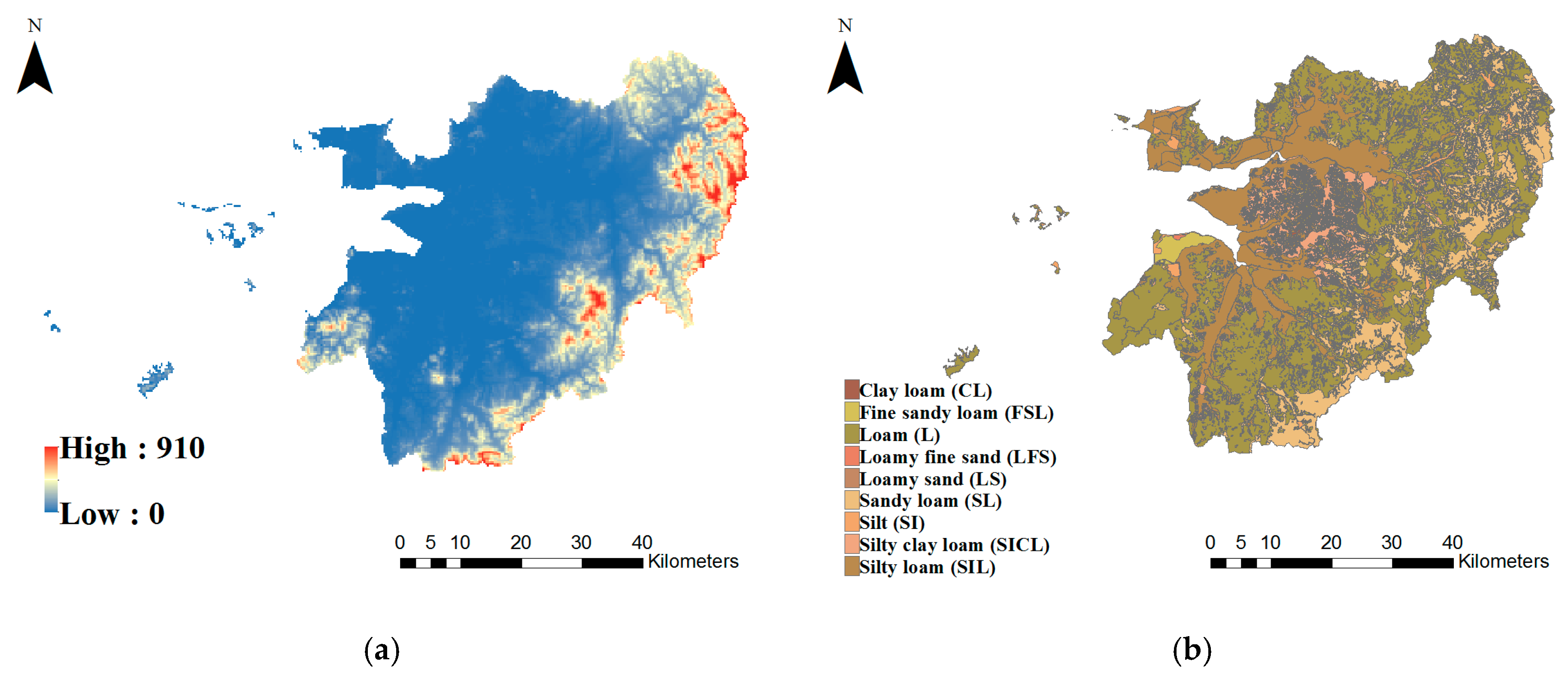
Neitsch et al. [16] recommended input parameters for setting up the SWAT model: meteorology (daily precipitation, wind speed, relative humidity, solar radiation, and maximum and minimum temperatures), topography (digital elevation model, DEM), soil type, and land use. Daily weather data (precipitation, wind speed, solar radiation, maximum and minimum temperatures, and relative humidity) at 12 monitoring stations (Gunsan, Jeonju, Buan, Jeongup, Muaksan, Iksan, Byeongsan, Jinbong, Gimje, Julpo, Tein, and Yeosan) across the study area were obtained from the Korea Meteorological Administration during 1997–2018. The specific site locations and temporal coverage varied for each dataset. A 350 × 350 m DEM (Figure 2a), acquired from the South Korean National Geographic Information Institute, was used to delineate streams, watersheds, and the longest possible flow path of streams during floods. Soil type is an important factor controlling both runoff and water quality processes, and land use is an important factor affecting runoff, evapotranspiration, and surface erosion in a watershed. Figure 2b shows the soil property input of the SWAT model (based on the values provided with the soil texture map from South Korean Soil Information System), which was classified based on the United Nations Food and Agricultural Organization and the United States Department of Agriculture charts for soil texture classification and supported by the SWAT soil database. The land use map (Figure 2c) was obtained from the National Geographic Information Institute and reclassified based on the SWAT database codes to represent land use according to the specific land cover types. Monthly streamflow and water quality data for January 2007 to December 2017 were obtained from the South Korean Water Resources Management System and Water Information System for calibration and validation.

2.2. Climate Change Scenarios and Future Climate Changes

Global climate models (GCMs) are generally the primary models used for constructing future climate change scenarios, and they provide the basis for assessing climate change on all scales. GCMs can provide the six major variables (precipitation, maximum temperature, minimum temperature, wind speed, solar radiation, and relative humidity) that are needed for modeling [12]. However, studies rarely use GCM outputs directly due to the significant errors in GCM historical simulations [17]. Therefore, it is important to bias-correct raw climate model outputs. We used the high-resolution RCP 4.5 and RCP 8.5 climate change scenario data (precipitation, maximum/minimum temperature, relative humidity, and wind speed) of the six GCM models (BCC-CSM1–1, CanESM2, GFDL-ESM2G, HadGEM2-CC, INM-CM4, and MIROC-ESM; Table 1) were obtained from the South Korean APEC Climate Center. In the Saemangeum watershed, the scenario data were based on four Automated Synoptic Observation System (ASOS) weather stations (Gunsan, Jeonju, Buan, and Jeongup) of the Korea Meteorological Administration in the Saemangeum watershed, and used the simple quantile mapping (SQM) downscaling method [18] for downscaling and bias correction. The SQM downscaling method uses non-parametric quantile mapping for downscaling and bias correction to produce reliable daily climate data for future periods [12].
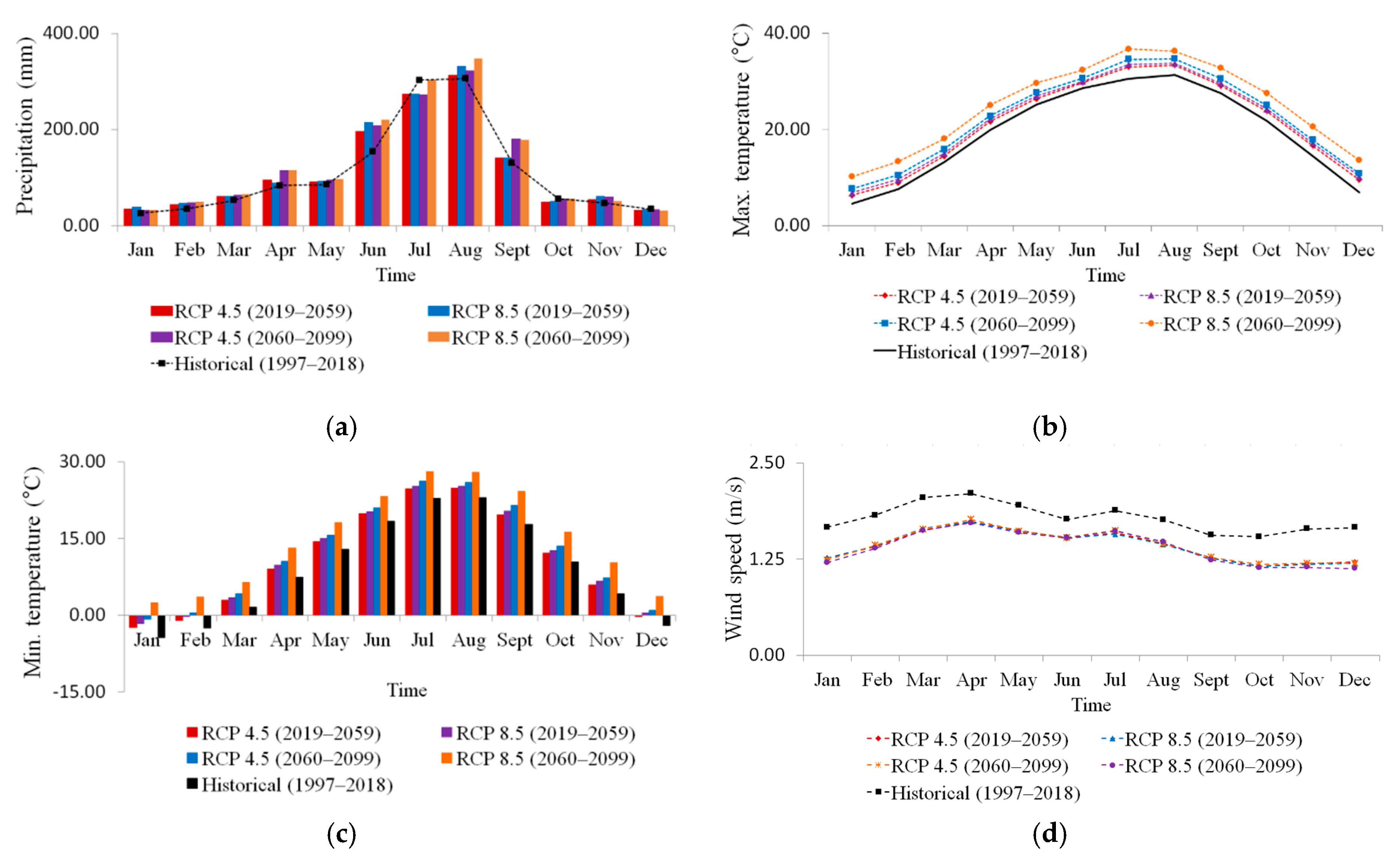
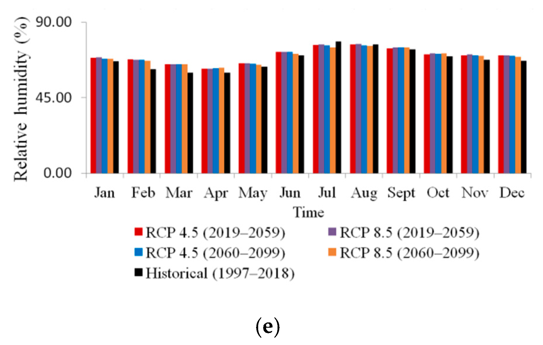
In this study, RCP 4.5 and RCP 8.5 climate change scenarios were used as the model input for predicting future trends of streamflow and NPS pollution in the Saemangeum watershed. Figure 3 shows the average values of the six GCMs from the main weather station (Jeonju) in the Saemangeum watershed, including the monthly average relative humidity, wind speed, daily maximum and minimum temperatures, and precipitation. Under the two climates change scenarios (RCP 4.5 and RCP 8.5) during the first time period (2019–2059), the future monthly average relative humidity is likely to increase by 2.1% and 2.2% relative to the baseline, respectively. During the second period (2060–2099) under the two climate change scenarios, the monthly average relative humidity is likely to increase by 1.6% and 2% relative to the baseline, respectively. Similarly, during 2019–2059 under RCP 4.5 and RCP 8.5, the monthly average wind speed is likely to decrease by 0.4 m/s relative to the baseline. During 2060–99, the monthly average wind speed under the two climate change scenarios is likely to decrease by 0.4 m/s.
When the climate changes, precipitation and temperature are the two dominant factors impacting streamflow and NPS pollution loads [19]. The annual average of daily maximum and minimum temperatures are likely to increase by 1.8 and 2.3 °C, and 1.7 and 2.3 °C relative to the baseline (1997–2018) during the first period (2019–2059) under RCP 4.5 and RCP 8.5, respectively. During the second period (2060–2099), the annual average of daily maximum and minimum temperatures are likely to rise by 3.1 and 5.4 °C, and 3.1 and 5.7 °C, respectively, relative to the baseline under the two climate change scenarios. During 2019–2059 under RCP 4.5 and RCP 8.5, the annual average precipitation is likely to increase by 70.9 and 119.3 mm, respectively, relative to the baseline. Similarly, during 2060–2099, the annual average precipitation under the two climate change scenarios is likely to increase by 170.6 and 233.8 mm, respectively. These results are summarized in Table 2, which shows that the trends in annual average of daily maximum/minimum temperatures and annual precipitation are similar to monthly average trends. Average temperature and precipitation increase under the two scenarios, with the sharpest increase in July and August. Accordingly, under RCP 4.5 and RCP 8.5 during the two periods, the monthly average of daily maximum and minimum temperatures sharply increase from 0.6 to 3.4 °C and 0.8 to 3.9 °C, respectively, in July and August. The changes in monthly average precipitation are similar to those in temperature: the precipitation increased significantly from −32.6 to 94.1 mm in July and August. This shows that the precipitation will be concentrated in summer.

2.3. Model Setup and Description

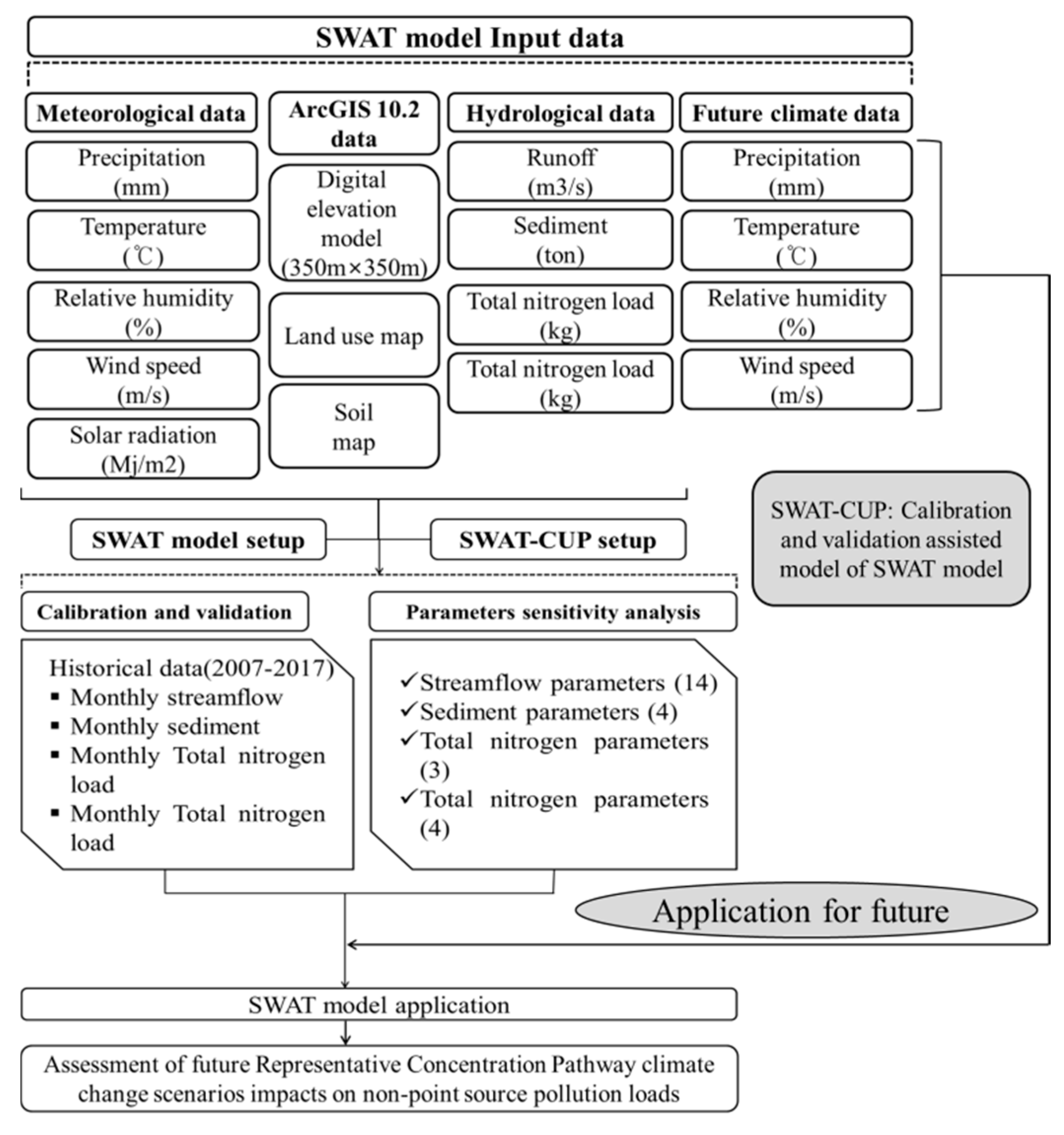
The SWAT (SWAT 2012) was used via the ArcSWAT interface embedded in ArcGIS 10.2 software (ESRI, Redlands, CA, US), and the model setup followed that described by Winchell et al. [5]. Figure 4 shows a diagram of the study process. The SWAT setup was divided into three segments: watershed delineation, hydrological response unit (HRU) definition, and input table writing. The input data for the SWAT model were applied at different levels of detail, including watershed, sub-watershed, and HRUs. The required spatial datasets were projected to the UTM Zone 52N with ArcGIS 10.2. The watershed was divided into eight Sub-Watersheds (Figure 1): Mangyeong sub-watershed (with Sub-Watersheds 1–6) and Dongjin sub-watershed (with Sub-Watersheds 7 and 8), and 91 HRUs in terms of land use, soil characteristics, and topography (using a DEM). During slope discretization, multiple slope discretization options were used and two slope classes were considered: below 10% and above 10%. Multiple HRUs were created for each sub-watershed using 10%, 10%, and 10% overlap for land use, soil type, and elevation, respectively. HRU delineation was based on watershed area threshold values [20] as criteria for the various hydrological conditions in the watershed and was simultaneously sufficiently limited to reduce the input data requirements and improve modeling efficiency [21]. Hydrological processes and water balance are important watershed parameters for SWAT simulation, as these must conform to what actually occurs in the watershed [4]. The accurate prediction of precipitation, surface runoff, base-flow, evapotranspiration, sediments, groundwater, and pesticide and nutrient movements were based on theoretical SWAT considerations as described by Neitsch et al. [16]. In this study, a water balance equation described by Neitsch et al. [16] (Equation (1)) was used for SWAT simulation of the hydrological component, and the modified universal soil loss equation in Equation (2) was used to estimate erosion and sediment yield.
S W t = S W 0 + i = 1 t ( R d a y Q s u r f E a W s e e p Q g w )
where SWt is the final soil water content (mm H2O), SW0 is the initial soil water content on day i (mm H2O), t is the time (days), Rday is the amount of precipitation on day i (mm H2O), Qsurf is the amount of surface runoff on day i (mm H2O), Ea is the amount of evapotranspiration on day i (mm H2O), Wseep is the amount of water entering the vadose zone from the soil profile on day i (mm H2O), and Qgw is the amount of return flow on day i (mm H2O).
S e d = 11.8 × ( Q s u r f × q p e a k × a r e a h r u ) 0.56 × K × C × P × L S × C F R G
where Sed is sediment yield per day (tons), Qsurf is the surface runoff volume (mm/ha), qpeak is the peak runoff rate (m3/s), areahru is the area of the HRU (ha), K is the soil erodibility factor, LS is the universal soil loss equation (USLE) topographic factor, C is the cover and management factor, P is the USLE support practice factor, and CFRG is the coarse fragment factor.

2.4. Model Calibration and Validation

The SWAT model was calibrated for monthly observed streamflow and water quality data from the Mangyeong and Dongjin sub-watersheds. The three water quality variables used in this study were based on the available data for water quality estimation: sediment, total nitrogen (TN), and total phosphorus (TP). The model simulation was performed for 11-year periods, with 2007–2010 datasets used for calibration and 2011–2017 for validation. The model warmup was performed using the first two years. Prior to model calibration, however, a sensitivity analysis was required to identify and rank input parameters according to the significance of their impacts on the model outputs, such as sediment and streamflow [16,22]. In addition, two statistical indices were used for the performance evaluation of the SWAT model simulation: the Nash–Sutcliffe efficiency (NSE) index and coefficient of determination (R2). The NSE index and R2 were calculated via Equations (3) and (4), respectively. The former determines the relative magnitude of the residual variance compared to measured data variance [23], and the latter describes the degree of collinearity between measured and simulated data [3].
NSE = 1   i = 1 N ( Q s , i   Q o , i ) 2 i = 1 N ( Q o , i   Q ¯ o ) 2
where N is the number of observations, Qs,i is the simulated value at time i, Qo,i is the observed value at time i, and Q ¯ o is the mean observed streamflow. NSE values range between –∞ and 1, with 1 being the optimal value.
R 2 = [ i = 1 N ( Q o , i   Q ¯ o )   ( Q s , i   Q ¯ s ) ] 2 i = 1 N ( Q o , i   Q ¯ o ) 2   i = 1 N ( Q s , i   Q ¯ s ) 2
where Q ¯ s is the simulated streamflow.
The sequential uncertainty fitting (SUFI-2) algorithm of the semi-automated calibration method in the SWAT calibration and uncertainty programs (SWAT-CUP) (Figure 5) was used for model calibration, and the boundary conditions (lower and upper boundaries) described in the SWAT user manual [17] were used. SUFI-2 uses the Latin hypercube one-factor-at-a-time analysis due to its combined strength in both local and global sensitivity analysis [24]. To obtain high-quality model simulation results [25], the most sensitive hydrological and water quality parameters were adjusted based on the available data from the six streamflow and water quality stations in the study area. The SUFI-2 is used to address all sources of uncertainties that may arise from input parameters and observed data, especially when the parameter range that matches the study area is unknown.
In this study, the Latin hypercube one-factor-at-a-time type of sensitivity analysis result is 6 of the 14 hydrologic parameters (CN2, SOL_AWC, SOL_K, ALPHA_BF, GW_DELAY, GWQMN, GW_REVAP, REVAPMN, ESCO, HRU_SLP, OV_N, SLSUBBSN, CH_N2, and CH_K2) were highly significant factors influencing the hydrological conditions in the Mangyeong and Dongjin sub-watersheds after 2000 iterations in the SWAT-CUP program (Table 1). Among the most sensitive parameters were soil conservation service runoff curve number (CN2), threshold depth of water in the shallow aquifer for return flow to occur (GWQMN), groundwater delay time (GW_DELAY), saturated hydraulic conductivity (SOL_K), available water capacity (SOL_AWC), and average slope steepness (HRU_SLP). These parameters were found to considerably influence the stream discharge of the watershed. This result agrees with those reported by Zhou et al. [24] and Mutenyo et al. [25]. Similarly, for water quality calibration, several parameters were used (Table 3). These parameters fell within the acceptable range after the adjustment. The USLE support practice factor (USLE_P) and USLE soil erodibility factor (USLE_K) in sediment, initial NO3 concentration in the soil layer (SOL_NO3) in TN, and phosphorus soil partitioning coefficient (PHOSKD) in TP were the most sensitive parameters.
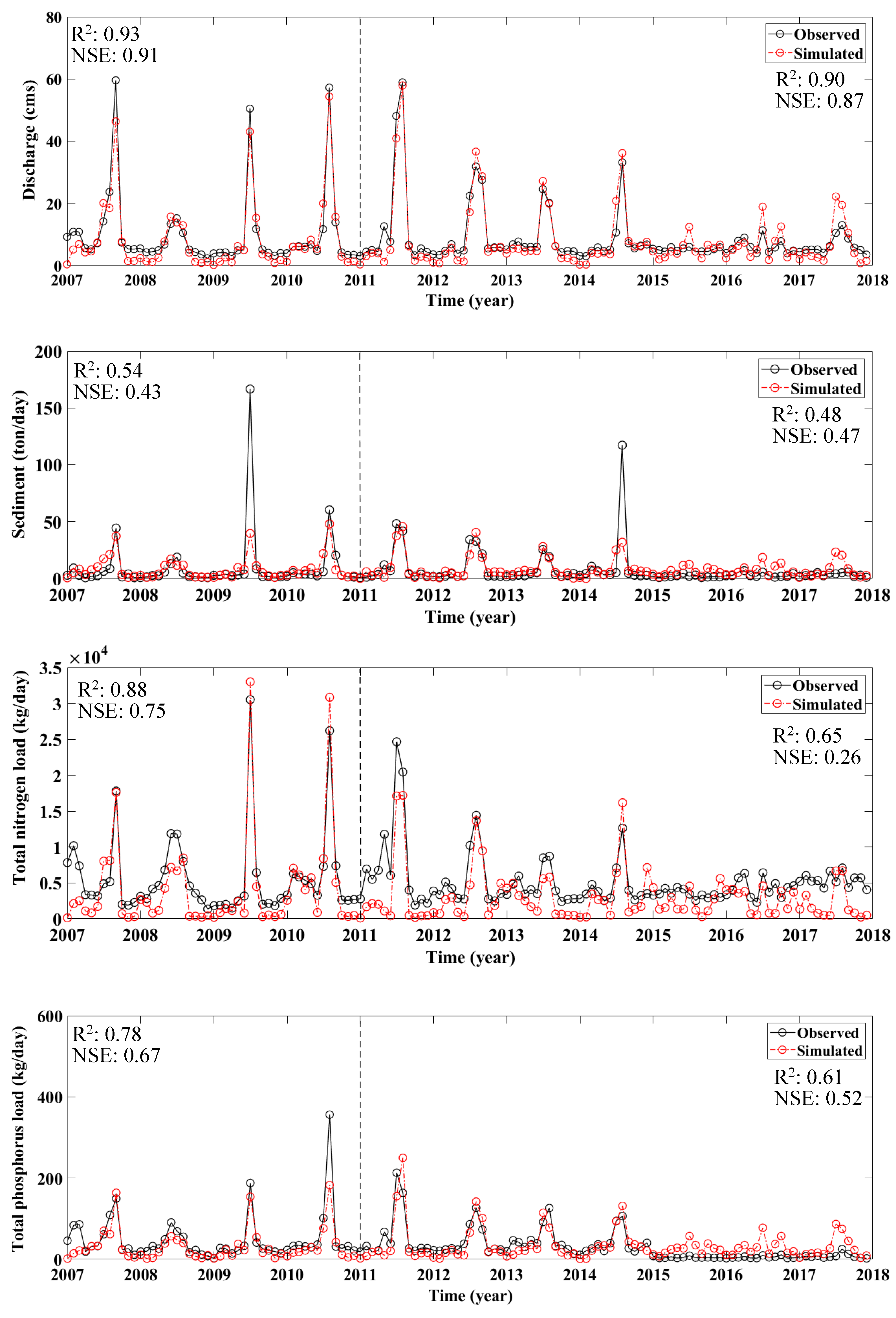
The SWAT model was calibrated for hydrological and water quality parameters using observed data from streamflow and water quality stations in Gosan (Sub-Watershed-1), Daecheon (Sub-Watershed-3), Soyang (Sub-Watershed-5), Jeonju-6 (Sub-Watershed-6) and Jeongup (Sub-Watershed-8). Table 4 to Table 5 compares the measured and simulated streamflow and NPS pollutant loads at the abovementioned five stations. The calibration and validation results show that for all the streamflow stations considered, the NSE values for the validation of Gosan and Jeongup stations were less than 0.5, whereas those of other stations were higher than 0.5. R2 values were higher than 0.5 for the calibration and validation periods. These lower objective function values can be attributed to the two upstream reservoirs (Gyeongcheon and Dae-a) that affect Gosan station and missing streamflow data of Jeongup station for the calibration period. Moriasi et al. [3] described a good calibration as one where the R2 is higher than 0.5 and the NSE value is positive. However, the overall results were consistent with the observed data as the models matched the precipitation pattern well and were able to capture the peak flows.
The calibration and validation results of water quality show that Gosan station (Sub-Watershed-1) had monthly average observed and simulated values of 3.1 and 4.9 t/day, 1848.6 and 1628.9 kg/day, and 26.6 and 19.8 kg/day for sediment, TN, and TP respectively. The results show a slight underestimation of these values. Correspondingly, the statistical performance evaluation of the models show that the only sediment had a positive NSE value and an R2 of more than 0.5 during the calibration period as suggested by Moriasi et al. [3]. TN and TP had R2 values of less than 0.5, and the NSE values were positive for all the pollutants in Sub-Watershed-1. The lower objective function values could be attributed to the impact on reservoirs downstream of the watershed. For Sub-Watershed-5, the average observed and simulated values of sediment, TN, and TP were 1.3 and 4.3 t/day, 1033.2 and 1334 kg/day, and 11.5 and 15.7 kg/day, respectively. Only sediment was overestimated, and TN and TP were accurately simulated. Accordingly, the statistical performance evaluation indicated that the NSE index and R2 values were greater than 0.5 for TN, whereas the NSE values for sediment and TP were −1.87 and 0.2, respectively, during validation. Similarly, the monthly average observed and simulated values of sediment, TN, and TP for Sub-Watershed-6 were 7.8 and 8.1 t/day, 5295.4 and 3360.6 kg/day, and 36.0 and 33.2 kg/day, respectively. Only sediment and TN had NSE values of below 0.5 during the validation period, and the rest of the water quality variables were accurately simulated. Accordingly, the statistical performance evaluation indicated that the NSE value was positive and R2 values were greater than 0.5. This indicates a good and acceptable model simulation for Sub-Watershed-6. The monthly average observed and simulated values of sediment, TN, and TP for Sub-Watershed-3 were 17.6 and 19.6 t/day, 8119.5 and 6751.4 kg/day, and 357.1 and 108.1 kg/day respectively. Only TP had R2 and NSE values of below 0.5, and the rest of the water quality variables were accurately simulated. The monthly average observed and simulated values of sediment, TN, and TP for Sub-Watershed-8 were 9.2 and 10.8 t/day, 804.7 and 761.5 kg/day, and 37.1 and 35.6 kg/day respectively. The NSE values, for both the calibration and validation, were positive for sediment, TN, and TP, indicating a good relative magnitude of the simulated variance compared to measured data variance. However, the R2 values of sediment and TN during calibration were less than 0.5, but there was an acceptable degree of collinearity among the measured and simulated data for sediment and TP during the validation period as the R2 value was greater than 0. Figure 6 depicts comparisons of the measured and simulated streamflow and water quality at Sub-Watershed-6.

3. Results and Discussion

The impacts of the future projection of potential climate change in precipitation and temperature on NPS pollution in the Saemangeum watershed were evaluated using SWAT. Using six GCM models (BCC-CSM1–1, CanESM2, GFDL-ESM2G, HadGEM2-CC, INM-CM4, and MIROC-ESM), outputs of RCP4.5 and RCP8.5 climate change scenarios were applied to the watershed and future projection results were arranged for two time periods (2010–2059, 2060–2099) using the baseline (1997–2018). After the evaluation of future precipitation and temperature, we used outputs of RCP 4.5 and RCP 8.5 climate change scenarios for each GCM model as the model input, and averaged the six results obtained to remove the climate change scenarios that contained large uncertainties. The impacts of future climate change on NPS pollution according to streamflow, sediment, and TN and TP loads in the Saemangeum watershed were assessed.
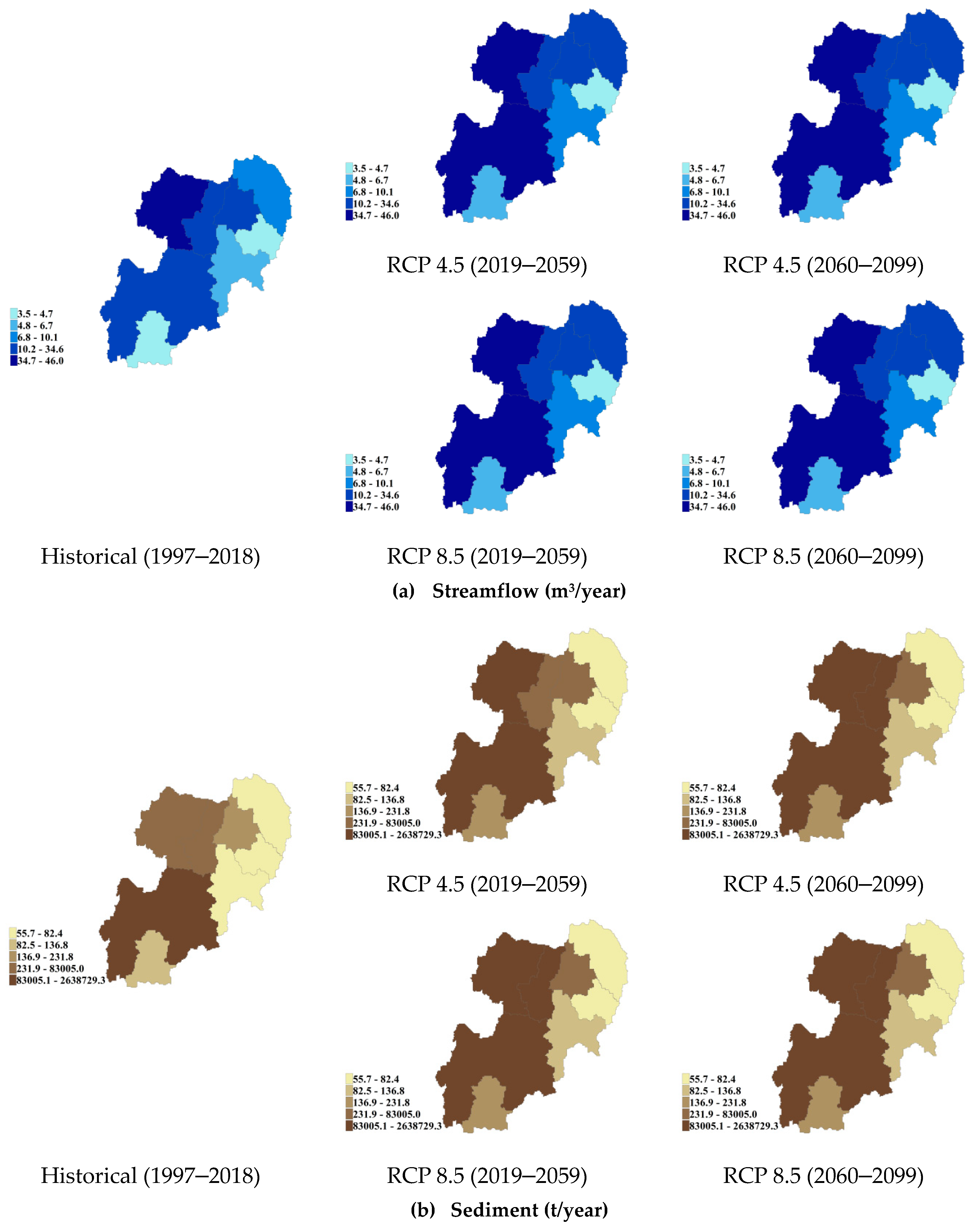
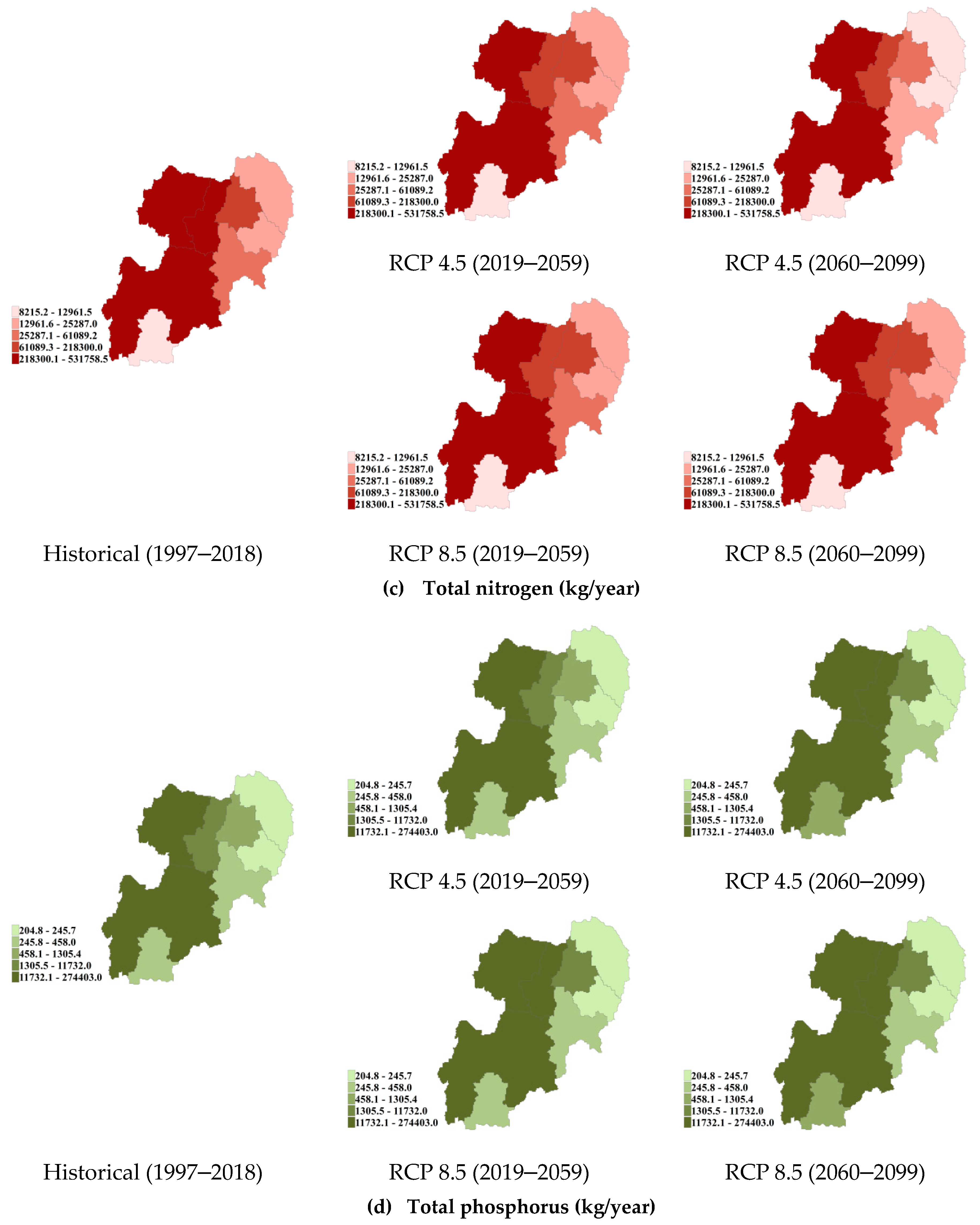
The spatial distribution of future streamflow and pollutant load during 2019–2059 and 2060–2099 under RCP 4.5 and RCP 8.5 relative to the baseline (1997–2017) were showed in Figure 7. With a gradual increase in annual precipitation and temperature during the two time periods (2019–2059 and 2060–2099) under RCP 4.5, Sub-Watershed-6 showed a considerable increase in annual average streamflow of 1.9 to 2.5 m3/s (28% to 38%), whereas other sub-watersheds showed increases of 0.5 to 1.7 m3/s (5% to 35%). The annual average sediment in Sub-Watershed-6 significantly increases by 20.7 to 28.3 t/year (25% to 34%), other sub-watersheds showed increases of 3.6 to 48.3 t/year (3% to 21%). Additionally, Sub-Watershed-6 showed a large decrease in annual average TN loads of −6720.6 to −9149.9 kg/year (−20% to −27%) and other sub-watersheds showed decreases in annual average TN loads of −1003.8 to −3899 kg/year (−7% to −23%). Sub-Watershed-5 showed a large increase in annual average TP load of 8.9 to 22.7 kg/year (4% to 11%) and Sub-Watershed-1 showed a large decrease of −27.2 to −36.1 kg/year (−11% to −15%) in annual average TP loads. Other sub-watersheds showed changes of −22.7 to 56.8 kg/year (−5% to 4%) in annual average TP loads.
In the same time period, under the RCP 8.5 scenario, sub-watershed-8 showed a large increase of 1.4 to 2.0 m3/s (30% to 43%) in annual average streamflow, while the other sub-watersheds showed increases of 0.9 to 2.5 m3/s (9% to 38%). In annual average sediment, Sub-Watershed-6 showed a large increase of 24.5 to 33.3 t/year (30% to 40%); other sub-watersheds showed increases of 8.8 to 61 t/year (6% to 26%). Sub-Watershed-6 showed a large decrease in annual average TN loads of −6106.4 to −7328.7 kg/year (−18% to −21%) and Sub-Watershed-1 annual average TP load decreases by −7.7 to −26.3 kg/year (−3% to −11%). Sub-Watershed-5 annual average TP load increases by 14.6 to 31.4 kg/year (7% to 15%), while annual average TN loads in the other sub-watersheds decrease by −473.4 to −3058.3 kg/year (−5% to −18%) and increases in annual average TP loads by 0 to 58.6 kg/year (0% to 13%).
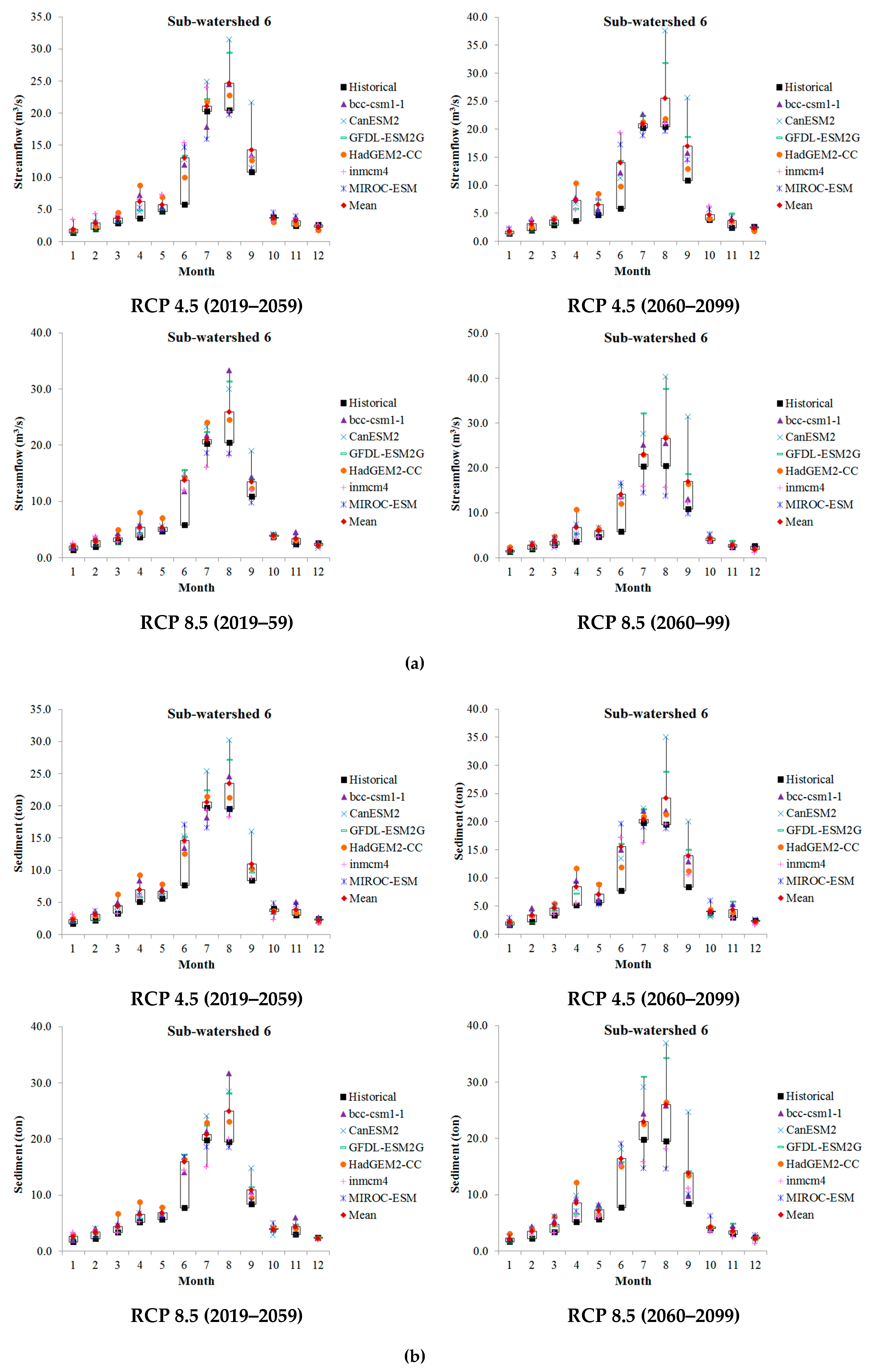
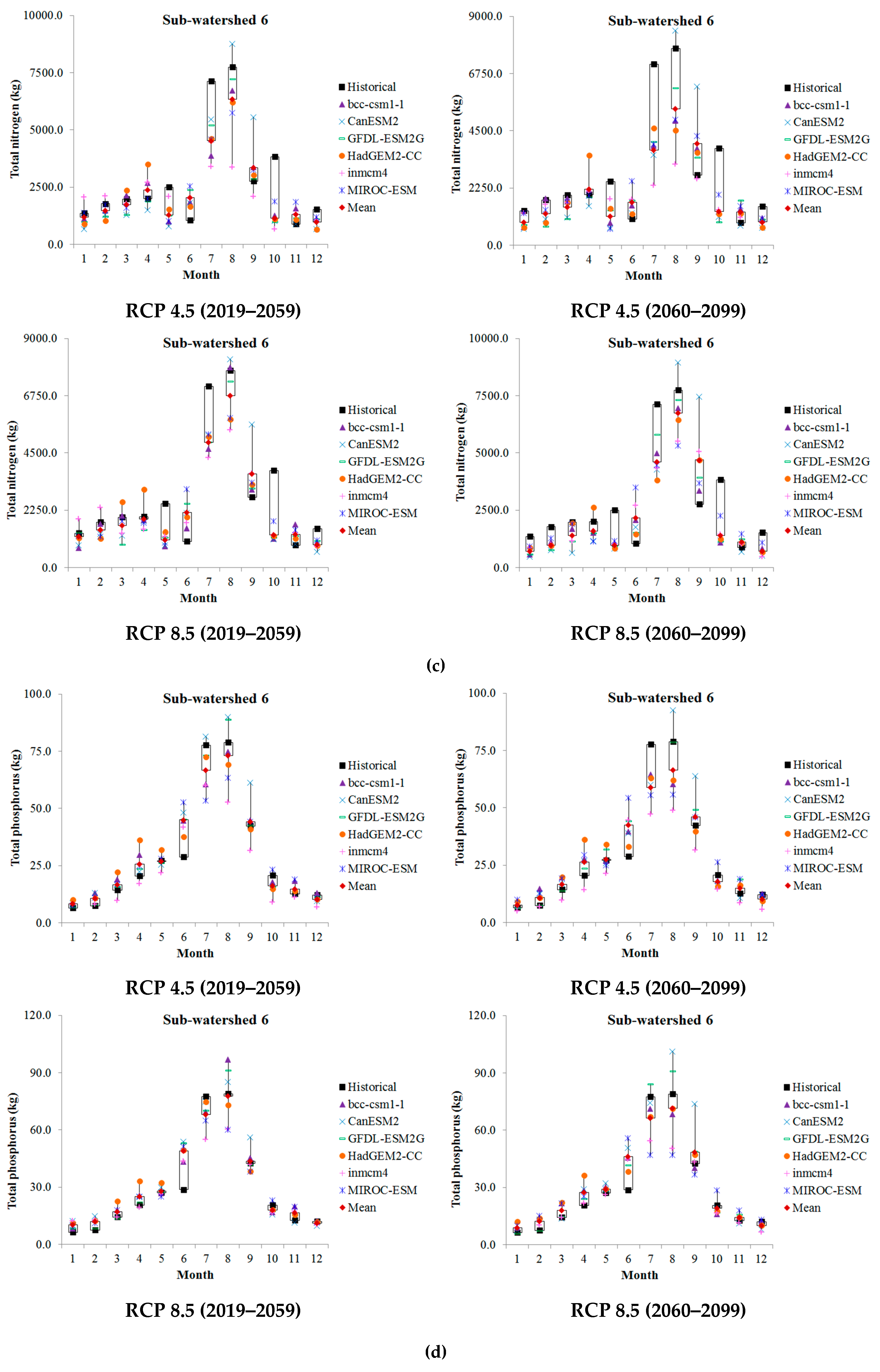
Table 6 shows the future monthly average streamflow and pollutant loads during the two time periods and under RCP 4.5 and RCP 8.5 relative to the baseline. Under RCP 4.5, monthly average streamflow in Sub-Watershed-6 is likely to considerably increase by 2.5 m3/s (37%), and the monthly average sediment is likely to increase by 2.3 ton/day (33%). The monthly average TN load in Sub-Watershed-6 is likely to largely decrease by −762.2 kg/day (–27%). In Sub-Watershed-3, the monthly average TP load is likely to decrease by −130.7 kg/day (−55%), whereas that in Sub-Watershed-5 is likely to increase by 1.9 kg/day (11%). Under RCP 8.5, the monthly average streamflow in Sub-Watershed-8 will considerably increase by 2 m3/s (43%), and monthly average sediment in Sub-Watershed-6 increases by 2.7 ton/day (39%). The monthly average TN load in Sub-Watershed-6 decreases by −611.1 kg/day (–21%). Finally, the monthly average TP load in Sub-Watershed-3 decreases by −127.3 kg/day (–53%), while that in Sub-Watershed-5 increases by 2.6 kg/day (15%). This indicates that the trends in average monthly and annual NPS pollution trends were similar. Figure 8a–d depict the changes in monthly streamflow, sediment, and TN and TP loads of Sub-Watershed-6 under the two climate change scenarios. The average monthly precipitation, temperature, streamflow, and sediment gradually increase. The monthly average TN and TP loads decrease overall, with the most significant decline occurring in July or August because vegetation under high-temperature conditions increases the absorption rates of nitrogen and phosphorus, i.e., continual increases in temperature will result in decreased TN or TP loads.
Climate change is one of the main factors affecting NPS pollution. Precipitation in particular has the greatest influence on streamflow and sediment, whereas temperature influences nitrogen and phosphorus concentrations in surface water. Therefore, regional impacts of climate change affect NPS pollution by changing the nitrogen and phosphorus loads in streamflow, which are also impacted by changes in the evaporation rate [20]. The future decrease of TN and TP loads in the target watershed may be associated with the gradual increase in precipitation and temperature which will increase the absorption rate of nitrogen and phosphorus by vegetation. The most significant decrease of TN and TP loads occurred in summer since vegetation in farmland under high-temperature conditions increases the absorption rates of nitrogen and phosphorus. Furthermore, according to the Saemangeum watershed land use map, upstream parts of the Mangyeong and Dongjin watersheds are covered by forests, and the downstream parts are mostly covered by agricultural land. A large amount of sediment flows into the river due to the increase in precipitation. This proves that climate change is one of the main factors affecting NPS pollution. Precipitation, in particular, has the greatest influence on streamflow and sediment, whereas temperature influences nitrogen and phosphorus concentrations in surface water. The results of this study show the potential to support the effective control of NPS pollution in the target watershed management under climate change scenarios.

4. Conclusions

In this study, we analyzed the impact of climate change on NPS pollution loads on a large spatial scale in the Saemangeum watershed under RCP climate change scenarios for an 81-year period (2019–2099) by applying SWAT modeling. These scenarios were obtained from the South Korean APEC Climate Center using the SQM downscaling method. The watershed was divided into the Mangyeong and Dongjin sub-watersheds. To adequately and accurately simulate runoff and water quality over a large area, we used the SUFI-2 algorithm of the semi-automated calibration method interfaced in SWAT-CUP for calibration and validation. The model satisfactorily simulated the streamflow with positive NSE index values and R2 > 0.5. However, the two climate change scenarios (RCP 4.5 and RCP 8.5) predicted gradual increases of 70.9 to 233.8 mm (5.4% to 17.8%) in annual precipitation and 1.7 to 5.7 °C (18.7% to 62.6%) increases in temperature during the two time periods (2019–2058 and 2059–2099).
After the evaluation of future precipitation and temperature, we selected the RCP 4.5 and RCP 8.5 climate change scenarios of each GCM model as the model input and averaged the six results obtained to remove the climate change scenarios containing large uncertainties. The annual average streamflow is likely to increase by 5% to 43% relative to the baseline (1997–2018), and the annual average sediment increases by 3% to 40%. The annual average TN loads decrease by −5% to −27%, while the annual average TP loads change by −15% to 15% relative to baseline in six Sub-Watersheds. The results for the two time periods under RCP 4.5 and RCP 8.5 show that monthly average streamflow increases by 6% to 43% relative to the baseline in six Sub-Watersheds. The monthly average sediment increases by 4% to 39%, and the monthly average TP loads change by −55% to 15%. Finally, the monthly average TN loads were likely to decrease by −5% to −27%. This shows that the trends in average monthly NPS pollution are similar to annual trends; as precipitation and temperature increase, streamflow and sediment increase overall, whereas the TN and TP load decrease overall. High temperatures, therefore, increase the evaporation rate and absorption rate of nitrogen and phosphorus, resulting in decreases TN and TP loads. We conclude that NPS pollutant loads are sensitive to RCP climate change scenarios. Therefore, future NPS pollutant loads in the Saemangeum watershed should be managed according to different climate change scenarios.

Author Contributions

T.L. and G.K. conceived and designed the experiments; T.L. performed the experiments; T.L. and G.K. analyzed the data; G.K. supervision experiments; T.L. wrote the paper.

Funding

This research was funded by Korea Environment Industry & Technology Institute (KEITI) through Advanced Water Management Research Program of the Korea Ministry of Environment (Grant No. 83067).

Conflicts of Interest

The authors declare no conflict of interest.

References

  1. Korea Meteorological Administration (KMA). Climate Change Projection Report on Korean Peninsula, Seoul, Republic of Korea. 2012. Available online: http://www.climate.go.kr/home/ (accessed on 31 December 2012).
  2. Ouyang, W.; Hao, F.H.; Wang, X.I. Regional Nonpoint source organic pollution modeling and critical area identification for watershed best environmental management. Water Air Soil Pollut. 2008, 187, 251–261. [Google Scholar] [CrossRef]
  3. Moriasi, D.N.; Arnold, J.G.; Van Liew, M.W.; Bingner, R.L.; Harmel, R.D.; Veith, T.L. Model evaluation guidelines for systematic quantification of accuracy in watershed simulations. Trans. Am. Soc. Agric. Biol. Eng. 2007, 50, 885–900. [Google Scholar]
  4. Yasin, H.Q.; Clemente, R.S. Application of SWAT model for hydrologic and water quality modeling in Thachin River Basin, Thailand. Arab J. Sci. Eng. 2014, 39, 1671–1684. [Google Scholar] [CrossRef]
  5. Winchell, M.; Srinivasan, R.; Luzio, M.D.; Arnold, J. ArcSWAT Interface for SWAT 2009 USDA Agricultural Research Service. Texas A&M Blackland Research Center: Temple, Texas, 2010. Available online: https://swat.tamu.edu/media/114647/2014-brazil-swat-conference-proceedings-secured.pdf (accessed on 30 July 2014).
  6. Gassman, P.W.; Reyes, M.R.; Green, C.H.; Arnold, J.G. The soil and water assessment tool: Historical development, applications, and future research directions. Trans. Am. Soc. Agric. Biol. Eng. 2017, 50, 1211–1250. [Google Scholar] [CrossRef]
  7. Choi, K.S.; Lee, S.G.; Jang, J.R. Vegetative filter strip (vfs) applications for runoff and pollution management in the Saemangeum area of Korea. J. Irrig. Drain. 2016, 65, 168–174. [Google Scholar] [CrossRef]
  8. Woo, H.J.; Jang, T.; Choi, J.K.; Son, J.K. Prioritizing sub-watersheds for non-point source pollution management in Saemangeum watershed using AHP technique. J. Korean Soc. Rural Plan. 2015, 21, 101–112. [Google Scholar] [CrossRef]
  9. Oh, C.; Cho, J.; Choi, J.; Cho, Y. Prediction of desalination time of Saemangeum reservoir. Irrig. Drain. 2016, 65, 221–229. [Google Scholar] [CrossRef]
  10. Kim, M.S.; Park, S.W.; Jang, N.J.; Kwak, D.H. Statistical analysis of water infrastructure characteristics: Case study of Saemangeum watershed. J. Water Resour. 2016, 43, 58–65. [Google Scholar] [CrossRef]
  11. Monica, N.; Choi, K.S. Temporal and spatial analysis of water quality in Saemangeum watershed using multivariate statistical techniques. Paddy Water Environ. 2016, 14, 3–17. [Google Scholar] [CrossRef]
  12. Cho, J.P.; Oh, C.; Choi, J.; Cho, Y. Climate change impacts on agricultural non-point source pollution with consideration of uncertainty in CMIP5. J. Irrig. Drain. 2016, 65, 209–220. [Google Scholar] [CrossRef]
  13. Gantidis, N.; Pervolarakis, M.; Fytianos, K. Assessment of the quality characteristics of two Lakes (Koronia and Volvi) of N. Greece. Environ. Monit. Assess. 2007, 125, 175–181. [Google Scholar] [CrossRef] [PubMed]
  14. Arnold, J.G.; Moriasi, D.N.; Gassman, P.W.; Abbaspour, K.C.; White, M.J.; Srinivasan, R.; Santhi, C.; Harmel, R.D.; Griensven, A.; Van Liew, M.W.; et al. SWAT: Model use, calibration, and validation. Trans. Am. Soc. Agric. Biol. Eng. 2012, 55, 1491–1508. [Google Scholar]
  15. Won, J.S.; Kim, S.W. ERS SAR Interferometry for Tidal Flat DEM. Proc. of FRINGE 2003 Workshop. Frascati, Italy, 2003. Available online: http://adsabs.harvard.edu/abs/2004ESASP.550E..16W (accessed on 5 December 2003).
  16. Neitsch, S.L.; Arnold, J.G.; Kiniry, J.R.; Williams, J.R. Soil and Water Assessment Tool Theoretical Documentation Version 2009. Texas Water Resources Institute, 2011. Available online: http://hdl.handle.net /1969.1/128050 (accessed on 1 September 2011).
  17. Ravichandran, S. Hydrological influences on the water quality trends in Tamiraparani basin, South India. Environ. Monit. Assess. 2003, 87, 293–309. [Google Scholar] [CrossRef]
  18. Cho, J.; Cho, W.; Jung, I. Statistical Downscaling Toolkit for Climate Change Scenario Using Non Parametric Quantile Mapping. 2018. Available online: https://cran.r-projectorg/web/packages/rSQM/.index.html (accessed on 14 February 2016).
  19. Wang, Y.; Bian, J.M.; Zhao, Y.S.; Tang, J.; Zhuo, J. Assessment of future climate change impacts on nonpoint source pollution in snowmelt period for a cold area using SWAT. Sci. Rep. 2018, 8, 2402. [Google Scholar] [CrossRef]
  20. Mekong River Committee. Decision Support Framework-SWAT and IQQM Models. 2004, p. 11. Available online: https://www.riob.org/en/file/264414/download?token=bzMrPwUO (accessed on 20 March 2004).
  21. Qiu, Z.; Wang, L. Hydrological and water quality assessment in a suburban watershed with mixed land uses using the SWAT model. J. Hydrol. Eng. 2014, 19, 816–827. [Google Scholar] [CrossRef]
  22. Abbaspour, K.C.; Yang, J.; Maximov, I.; Siber, R.; Bogner, K.; Mieleitner, J.; Zobrist, J.; Srinivasan, R. Modeling hydrology and water quality in the pre-alpine/alpine Thur watershed using SWAT. J. Hydrol. 2007, 333, 413–430. [Google Scholar] [CrossRef]
  23. Nash, J.E.; Sutcliffe, J.V. River flow forecasting through conceptual model. Part 1—A discussion of principles. J. Hydrol. 1970, 10, 282–290. [Google Scholar] [CrossRef]
  24. Zhou, J.; Liu, Y.; Guo, H.; He, D. Combining the SWAT model with sequential uncertainty fitting algorithm for streamflow prediction and uncertainty analysis for the Lake Dianchi Basin, China. Hydrol. Process. 2012, 28, 521–533. [Google Scholar] [CrossRef]
  25. Mutenyo, I.; Nejadhashemi, A.P.; Woznicki, S.A.; Giri, S. Evaluation of SWAT performance on a mountainous watershed in tropical Africa. Hydrol. Curr. Res. 2013, S14, 001. [Google Scholar]
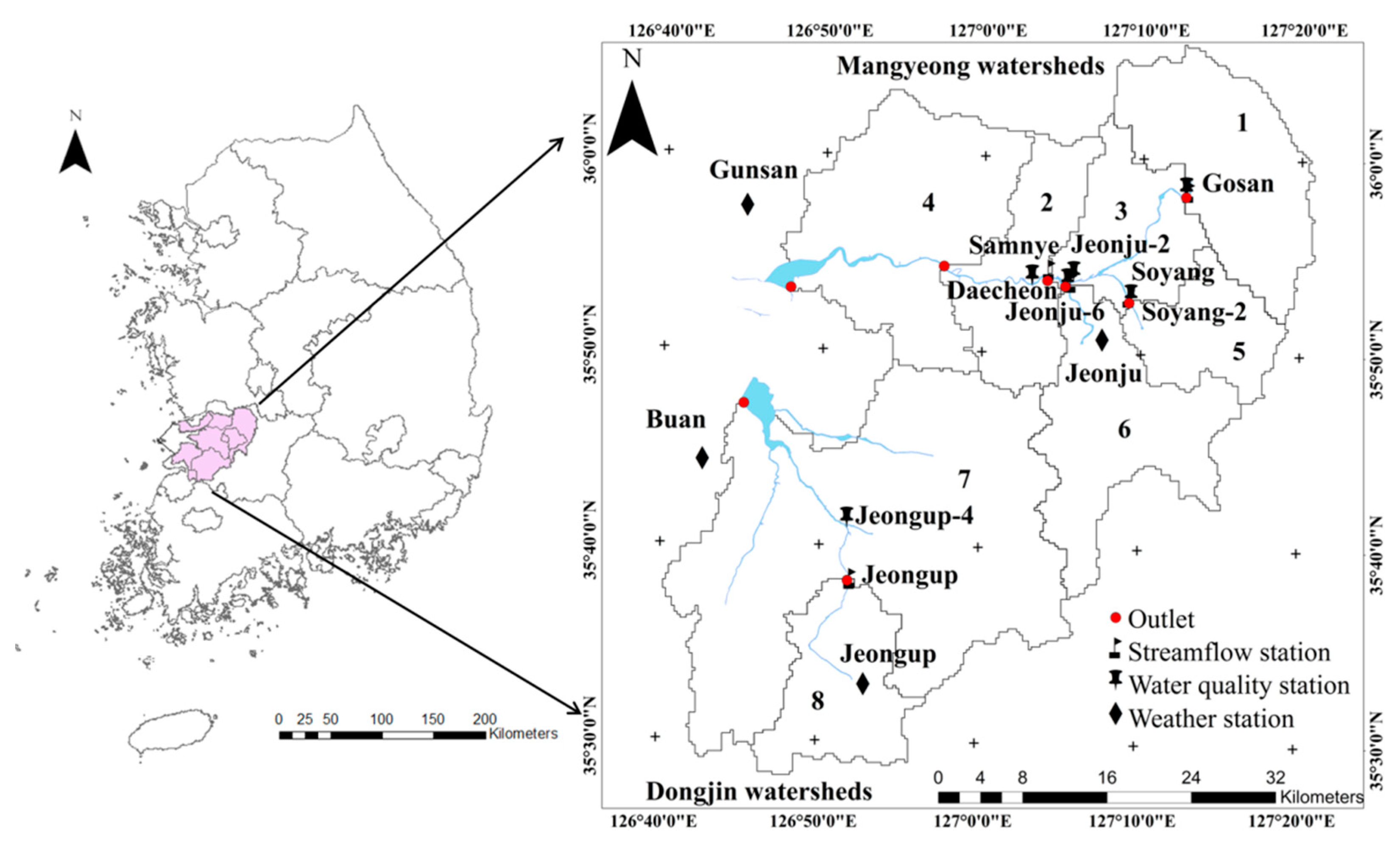
Figure 1. Location of the study area in the Saemangeum watershed and sampling points.
Water 11 01982 g001
Figure 2. Input data from the study area: (a) digital elevation model (DEM), (b) soil texture map, and (c) land use map (Source: https://www.ngii.go.kr).
Water 11 01982 g002aWater 11 01982 g002b
Figure 3. Characteristics of future seasonal (a) precipitation, (b) maximum temperature, (c) minimum temperature, (d) wind speed, and (e) relative humility under two climate change scenarios.
Water 11 01982 g003aWater 11 01982 g003b
Figure 4. Diagram of the study process.
Water 11 01982 g004
Figure 5. Soil and water assessment tool calibration and uncertainty programs (SWAT-CUP) model structure (PSO: Parameter Solutions; SUFI2: Sequential Uncertainty Fitting; MCMC: Markov Chain Monte Carlo; PraSol: Particle Swarm Optimization; GLUE: Generalized Likelihood Estimation).
Water 11 01982 g005
Figure 6. Calibration and validation results of streamflow and water quality in Sub-Watershed-6.
Water 11 01982 g006
Figure 7. Spatial distribution of future (a) streamflow, (b) sediment, (c) total nitrogen, and (d) phosphorus loads during two time periods (2019–59 and 2060–99) relative to baseline (1997–2018) under two climate change scenarios: RCP 4.5 and RCP 8.5.
Water 11 01982 g007aWater 11 01982 g007b
Figure 8. The ranges in future monthly (a) streamflow, (b) sediment, (c) TN load, and (d) TP load for Sub-Watershed-6 the Saemangeum watershed under the representative concentration pathway (RCP) climate change scenarios compared with the baseline.
Water 11 01982 g008aWater 11 01982 g008b
Table 1. Information about the global climate models (GCMs) used in this study.
No.GCMResolution (Degree)Institution
1BCC-CSM1–1-M1.125 × 1.122Beijing Climate Center, China Meteorological Administration
2HadGEM2-CC1.875 × 1.250Met Office Hadley Centre
3INM-CM42.000 × 1.500Institute for Numerical Mathematics
4GFDL-ESM2G2.500 × 2.023Geophysical Fluid Dynamics Laboratory
5CanESM22.813 × 2.791Canadian Centre for Climate Modelling and Analysis
6MIROC-ESM2.813 × 2.791Japan Agency for Marine-Earth Science and Technology, Atmosphere and Ocean Research Institute (The University of Tokyo), and National Institute for Environmental Studies
Table 2. Future changes of the annual averages of daily max/min temperature and annual precipitation at the Jeonju weather station.
Climate VariableBaseline
1997–2018
Scenario2019–20592060–2099
Sim.Var.Sim.Var.
Annual average of daily max. temperature (°C)19.3RCP 4.521.11.822.43.1
RCP 8.521.62.324.75.4
Annual average of daily min. temperature (°C)9.1RCP 4.510.81.712.23.1
RCP 8.511.42.314.85.7
Annual precipitation (mm)1315.2RCP 4.51386.170.91485.8170.6
RCP 8.51434.4119.31548.9233.8
Note: Sim.: simulation value; Var.: variety value.
Table 3. Selected input hydrological and water quality parameters for model calibration.
ParameterDefinitionLBUB
StreamflowCN2Soil conservation service runoff curve number for moisture condition II3598
GWQMNThreshold depth of water in shallow aquifer required for return flow to occur (mm H2O)05000
SOL_KSaturated hydraulic conductivity (mm/h)02000
SOL_AWCAvailable water capacity01
HRU_SLPAverage slope steepness00.6
GW_DELAYGroundwater delay time (days)0500
SedimentUSLE_PUniversal soil loss equation support practice factor0.080.54
USLE_KUniversal soil loss equation soil erodibility factor00.65
CH_COV1Channel erodibility factor00.6
CH_COV2Channel cover factor01
TNCMNRate factor for humus mineralization of active organic nitrogen0.0010.003
SOL_NO3Initial NO3 concentration in the soil layer0100
BIOMIXBiological mixing efficient01
TPPPERCOPhosphorus percolation coefficient1017.5
ERORGPOrganic P enrichment ratio05
SOL_ORGPInitial organic P concentration in surface soil layer0100
PHOSKDPhosphorus soil partitioning coefficient100200
Note: LB: lower boundary; UB: upper boundary.
Table 4. Performance statistics of streamflow and water quality simulation.
Sub-WatershedStatisticsFlows
(m3/s)
Sediment
(ton/day)
TN Loads
(kg/day)
TP Loads
(kg/day)
Cali.Vali.Cali.Vali.Cali.Vali.Cali.Vali.
1R20.660.50.680.420.410.240.450.18
NSE0.620.480.520.370.380.160.420.17
3R20.910.840.840.630.820.630.370.28
NSE0.900.840.810.590.720.57−0.60.07
5R20.860.910.560.330.710.640.490.78
NSE0.850.87−0.18−1.870.700.60.480.25
6R20.930.900.540.480.880.650.780.61
NSE0.910.870.430.470.750.260.670.52
8R20.510.680.40.620.350.510.490.62
NSE0.50.530.30.560.30.380.450.62
Note: Cali.: calibration period (2007–2010); Vali.: validation period (2011–2017).
Table 5. Comparative results of streamflow and water quality simulation.
Sub-WatershedFlow
(m3/s)
Sediment
(t/day)
TN Loads
(kg/day)
TP Loads
(kg/day)
Obs.Sim.Obs.Sim.Obs.Sim.Obs.Sim.
1109.53.14.91848.61628.926.619.8
321.220.517.619.68119.56751.4357.1108.1
52.73.21.34.31033.2133411.515.7
68.98.07.88.15295.43360.63633.2
82.33.19.210.8804.7761.537.135.6
Note: Obs.: observation value; Sim.: simulation value.
Table 6. Monthly average streamflow, sediment, and total nitrogen (TN) and total phosphorus (TP) loads under two representative concentration pathway (RCP) climate changes scenarios.
Sub-WatershedVariableBaseline
1997–2018
Scenario2019–20592060–2099
Sim.Var.Sim.Var.
1Streamflow
(m3/s)
10RCP 4.510.66%11.414%
RCP 8.510.99%11.717%
Sediment
(t/km2/day)
5.2RCP 4.55.44%5.812%
RCP 8.55.68%6.117%
TN
(kg/km2/day)
1405RCP 4.51134.2−19%1080.0−23%
RCP 8.51158.8−18%1150.2−18%
TP
(kg/km2/day)
20.5RCP 4.517.5−15%18.2−11%
RCP 8.518.2−11%19.8−3%
3Streamflow
(m3/s)
24.4RCP 4.528.015%30.425%
RCP 8.528.517%30.726%
Sediment
(t/km2/day)
19.3RCP 4.521.712%23.321%
RCP 8.522.517%24.426%
TN
(kg/km2/day)
6303.6RCP 4.55475.0−13%5091.3−19%
RCP 8.55575.2−12%5422.0−14%
TP
(kg/km2/day)
239.3RCP 4.5108.6−55%113.5−53%
RCP 8.5112.0−53%119.0−50%
5Streamflow
(m3/s)
3.5RCP 4.54.014%4.426%
RCP 8.54.014%4.425.7%
Sediment
(t/km2/day)
4.6RCP 4.54.97%5.315%
RCP 8.55.111%5.520%
TN
(kg/km2/day)
1219.8RCP 4.51136.1−7%1056.9−13%
RCP 8.51143.4−6%1110.9−9%
TP
(kg/km2/day)
17.1RCP 4.517.84%19.011%
RCP 8.518.37%19.715%
6Streamflow
(m3/s)
6.7RCP 4.58.628%9.237%
RCP 8.58.628%9.339%
Sediment
(t/km2/day)
6.9RCP 4.58.625%9.233%
RCP 8.58.929%9.639%
TN
(kg/km2/day)
2869.7RCP 4.52309.7−20%2107.5−27%
RCP 8.52360.9−18%2258.6−21%
TP
(kg/km2/day)
29RCP 4.529.93%28.8−1%
RCP 8.531.48%30.97%
8Streamflow
(m3/s)
4.7RCP 4.55.926%6.436%
RCP 8.56.130%6.743%
Sediment
(t/km2/day)
11.4RCP 4.511.73%12.611%
RCP 8.512.16%13.418%
TN
(kg/km2/day)
756RCP 4.5693.5−8%684.4−9%
RCP 8.5710.6−6%716.6−5%
TP
(kg/km2/day)
38.2RCP 4.536.3−5%39.43%
RCP 8.538.20%43.113%
Note: Sim.: simulation value; Var.: percentage value of variety.