3.1. Site Information and Demand Data
Except for the concept of the zero-height dam, the other main thrust of this paper is on the methodology for the generation of inflow data. Nevertheless, basic information on the site and a set of specific data for downstream demands are also given, to highlight the manner in which the two main components of the present study (i.e., the concept of the zero-height dam and the methodology of generating inflow data) can be applied for the computation of reservoir active storage capacity.
The hydrologic basin upstream of the dam site under investigation is in North Western Peloponnisos, Greece, with an area of 1000 km
2. Actual discharge measurements are not available, but a time-series of monthly precipitation heights is available for the period of September 1974 to August 1995. These data have been collected near the hypothetical dam site. The precipitation data are given in
Table A1 of
Appendix A. It must be noted that neither the hydrology of the area nor the demand of water affects the applicability of the methodology proposed herein. Also, for analysis purposes, it is assumed that the surface run-off coefficient is equal to unity. Thus, the monthly precipitation data can be converted to inflow data (m
3/month) for the proposed dam site after multiplication with 10
−3 × 1000 × 1000
2 = 10
6.
Based on a preliminary investigation, it was determined that the demand must cover: (a) summer irrigation needs for 15,000 ha with an average monthly consumption of 2000 m
3/ha, i.e., 30 × 10
6 m
3/month, 50% of the summer consumption for April, May, September, and October, and 0% during the remaining months, (b) water supply for an urban area of 500,000 residents with mean daily consumption of 0.25 m
3 per capita, i.e., 500,000 × 0.25 × 30 = 3.75 × 10
6 m
3/month during the summer months and 50% of the above (i.e., 1.875 × 10
6 m
3/month) during the rest of the year, and (c) demand for hydro-power generation, which was estimated to be 8.224 × 10
6 m
3/month. The temporal distribution of the demands is given in
Table 4. It is noted that the specific values utilized herein can be covered by the flow rates even during the driest year of the available record.
3.2. Generation of Inflow Data
The stochastic generation of flow data has been the subject of intense investigation in the past (e.g., [
9,
10,
11,
12]). However, preliminary computations of required storage capacity for the available 21-year record revealed some interesting results, e.g., the computations shown in
Table A2 of
Appendix A produced a required storage capacity of 127.43 × 10
6 m
3 for a yearly inflow of 276.81 × 10
6 m
3, corresponding to the year 1991–1992. On the other hand, the required storage capacity for the year 1984–1985 was equal to 191.14 × 10
6 m
3, while the yearly inflow was 722.17 × 10
6 m
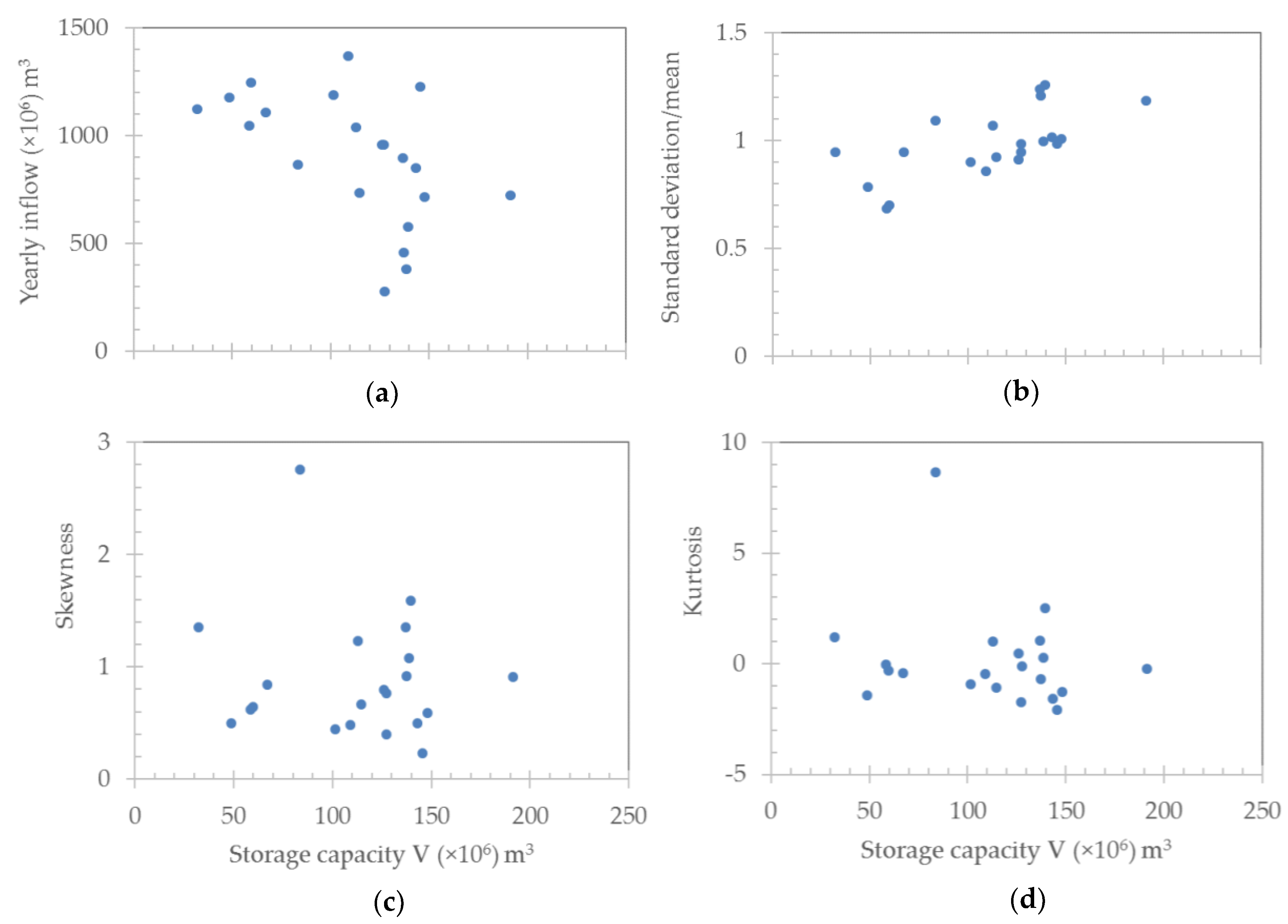
3. This implies that it is the monthly variations that primarily determine required storage capacity, and to a lesser extent the yearly values. Using the data from the 21 years of record, the computation of storage capacity for 1-year regulation did not reveal any correlation between storage capacity and yearly inflows or their important statistics, i.e., normalized standard deviation, skewness, and kurtosis. The results are shown in
Figure 2.
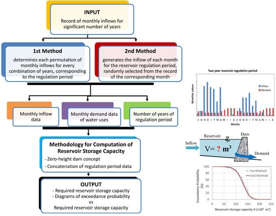
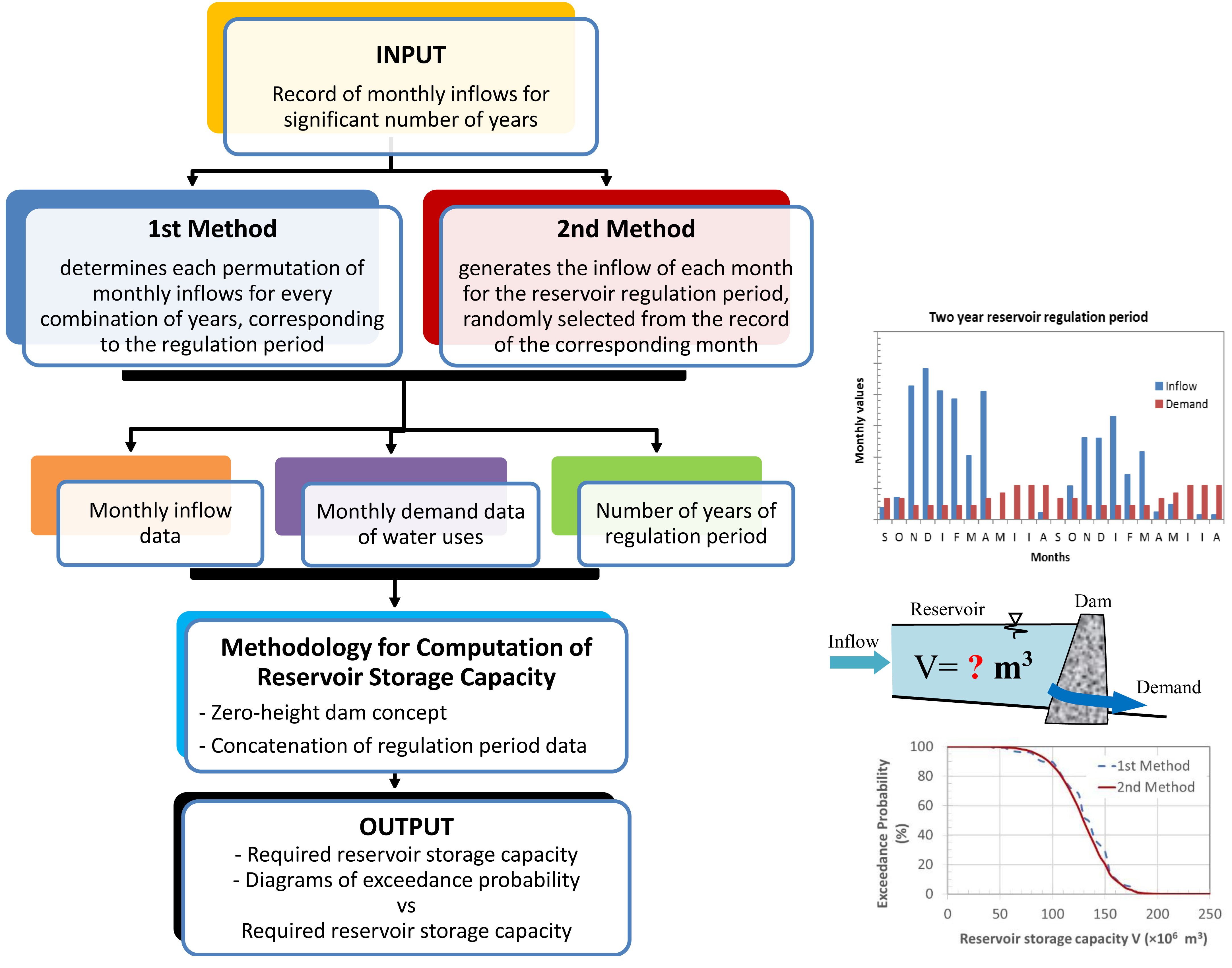
Hence, in this paper, a different approach was employed, especially in view of the fact that we seek to determine storage capacity for multi-year regulation. Thus, the generation of inflow data from the available record was performed using two different methods.
In the first method (hereafter called the First Method) we employed the following procedure:
We utilized the annual precipitation heights of the 21 hydrologic years and computed the average precipitation height for the combination of the 21 years per 1, 2, 3, 4, 5, and 6 years of the regulation period.
Subsequently, we performed all possible permutations of the years in each combination and computed the required reservoir capacity, with the methodology of
Section 2, to satisfy the prescribed demands.
The results of the analysis are summarized in
Table 5, where only the maximum reservoir storage capacities, from all values computed for each regulation period, are presented.
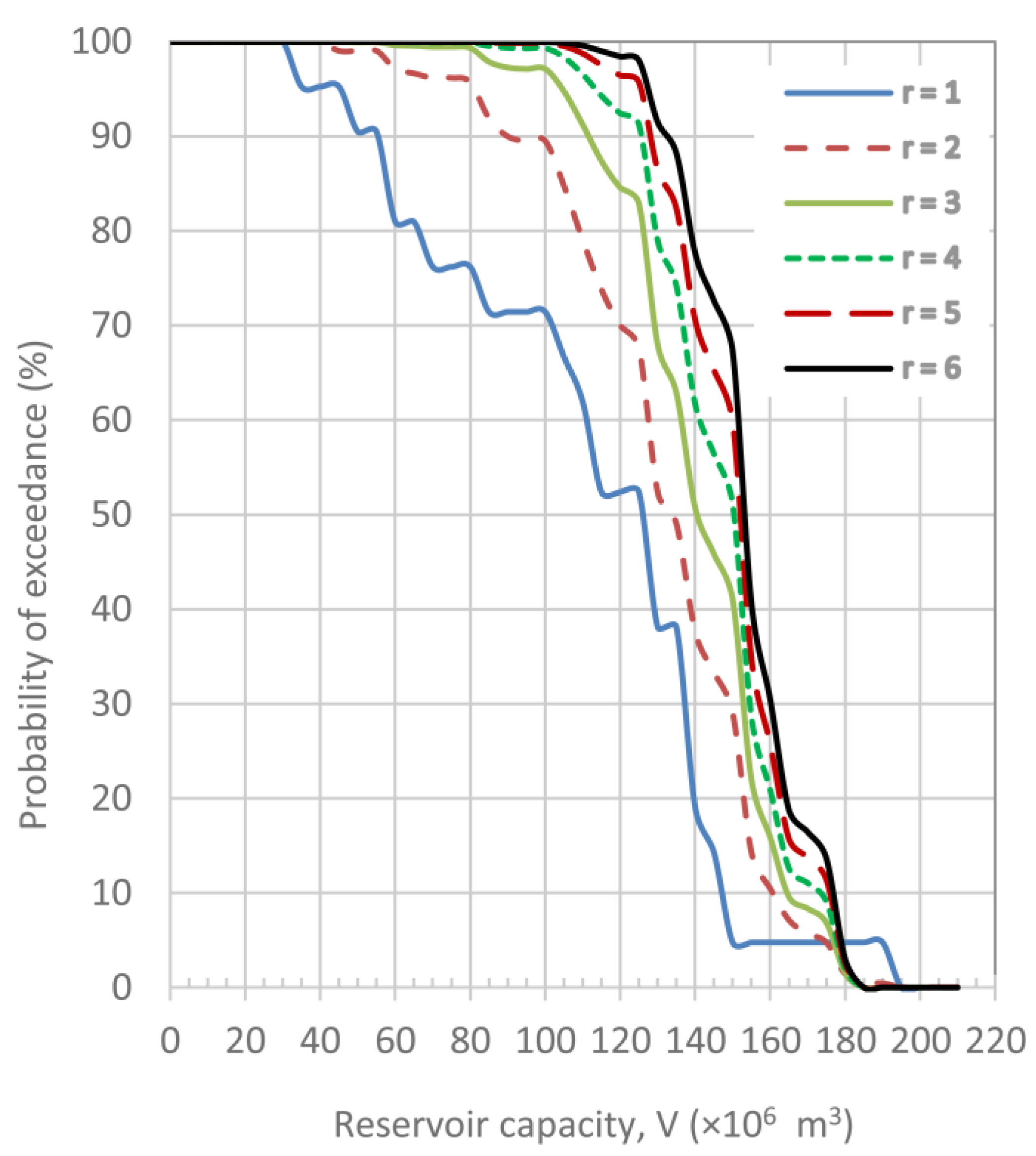
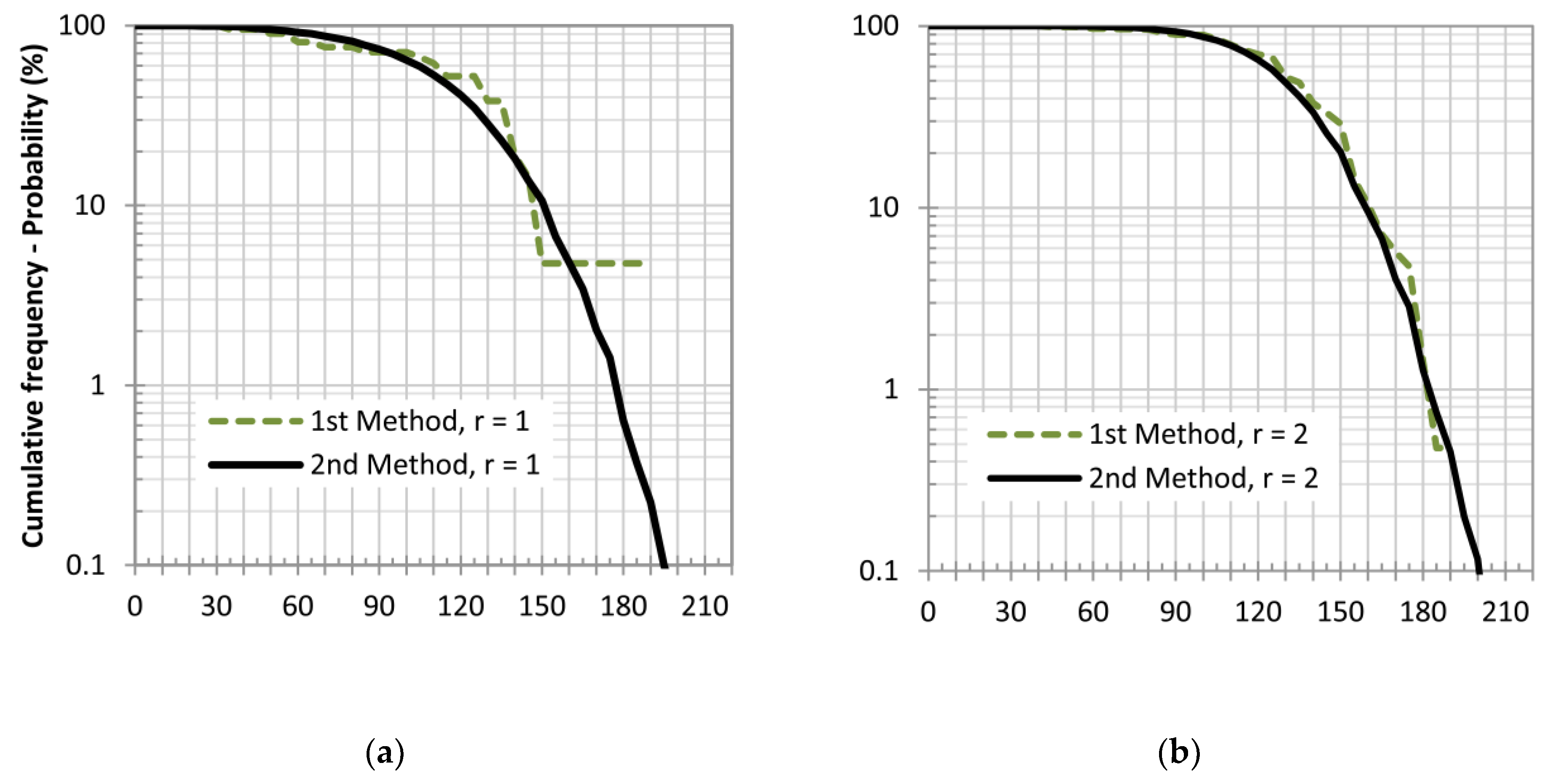
All the results, for each regulation period, are shown in
Figure 3, where the cumulative frequency of exceedance, interpreted as probability of exceedance for any given reservoir capacity, is plotted for regulation periods r = 1 to r = 6 years.
One can observe that the reservoir capacity increases with increasing regulation periods, up to a practically limiting value of 184.45 × 10⁶ m3. This limiting value has very small probabilities for regulation periods of 1 and 2 years and probabilities very close to zero for longer regulation periods. It can also be observed that the curves corresponding to r = 5 and r = 6 are practically the same; this leads to the conclusion that the reservoir capacity, as a function of the regulation period, will not increase for longer regulation periods.
A second approach for tackling the problem of inflow data generation (hereafter called the Second Method) was based on the generation of a random year consisting of random precipitation values for each month, corresponding to the available monthly values for the 21 hydrologic years. The procedure, for a regulation period of 1 year is as follows:
Twelve random integer numbers, R(I) with I = 1.12, were generated with values ranging from 1 to 21, which are the available hydrologic years of record.
For each value of R(I), the corresponding month and its inflow were selected through a FORTRAN Do loop of the form:
DO I = 1.12
I1 = 12 × (R(I) − 1) + I
F(I1) = MONTH (I1)
END DO
where MONTH(I1) contains, sequentially, the 12 × 21 = 252 values of inflow (see
Table A1) for 21 consecutive years. This procedure ensures that a random monthly inflow (for each specific month) of the random year will be selected.
For the year thus generated, the required reservoir capacity was computed.
The procedure was applied for the generation of 1,000,000 random hydrologic years and the computation of the corresponding required reservoir capacities. The sample represents the 13.6 × 10⁻⁹% of all possible cases, which are equal to 2112 = 7,355,827,511,386,641.
The extension of the method for a multiple-year regulation period, r, is accomplished in a similar manner except that the random numbers are generated for 12 × r months. The method was used for the computation of reservoir capacities with regulation periods of 2, 3, 4, 5, 6, 8, and 10 years. For each regulation period, 1,000,000 hydrologic years were generated except for the regulation period of 10 years, where 1,621,958 hydrologic years were generated. The maximum of all required values for the reservoir capacity is summarized in
Table 6.
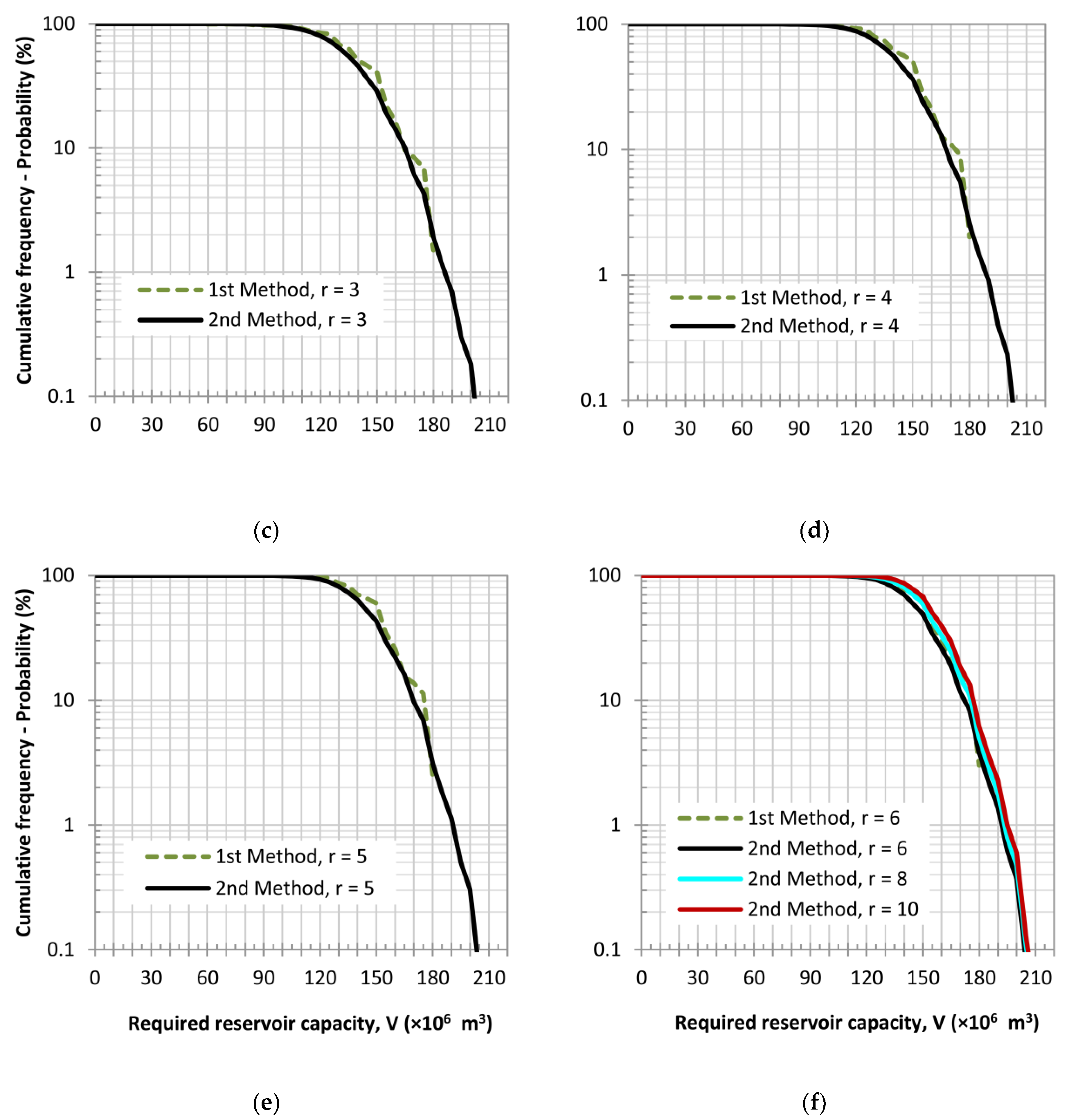
The results, from both methods and for each regulation period, are shown in
Figure 4, where the cumulative frequency of exceedance, interpreted as probability of exceedance for any given reservoir capacity, is plotted for regulation periods r = 1 to r = 10 years. For instance, if the selected regulation period of the reservoir under consideration is three years, the required storage capacity would be 173 × 10
6 m
3, 186 × 10
6 m
3, and 203 × 10
6 m
3 for 5%, 1%, and 0.1% probability of exceedance, respectively. The choice of the level of exceedance probability may be a matter of economic, social, and environmental factors; the lower the probability level the greater the reservoir storage capacity, hence the more expensive the project. These outcomes are necessary so that engineers may form alternative project budgets, which in turn are very significant to decision-makers for the final decision.
In summary, the First Method utilizes the combination of n = 21 years per k = 1, 2, 3, 4, 5, and 6 regulation years and subsequently performs all the permutations (k!) in each combination of k years, leading to a total of n!/(n − k)! cases. In the Second Method, hydrologic years were generated with inflow values for each month, randomly selected from the observed values for that month.
It is apparent from
Figure 4 that both methods give practically the same results. This was expected, since the First Method essentially produces results, which can be viewed as a subset of the results of the Second Method. Furthermore, the Second Method has the advantage of allowing for the manipulation of a greater volume of data with practically the same ease for short or long regulation periods. It also requires much shorter computation times, that did not exceed 2 min for each case examined. Therefore, the present findings imply that the proposed Second Method is very robust and is suggested for use.
All computations were performed via codes written in FORTRAN 77 and the diagrams were prepared with EXCEL 2016.


