Spatial Pattern Oriented Multicriteria Sensitivity Analysis of a Distributed Hydrologic Model


Abstract
1. Introduction
2. Materials
2.1. Satellite-Based Data
2.1.1. Leaf Area Index (LAI)
2.1.2. Actual Evapotranspiration (TSEB)
2.2. Hydrologic Model
3. Methods
3.1. Objective Functions Focusing on Spatial Patterns
3.1.1. Goodman and Kruskal’s Lambda
3.1.2. Theil’s Uncertainty Coefficient
3.1.3. Cramér’s V
3.1.4. Mapcurves
3.1.5. Empirical Orthogonal Functions
3.1.6. Fractions Skill Score
3.2. Latin Hypercube Sampling One-Factor-at-a-Time Sensitivity Analysis
4. Results
4.1. Exploration of Spatial Metrics Characteristics
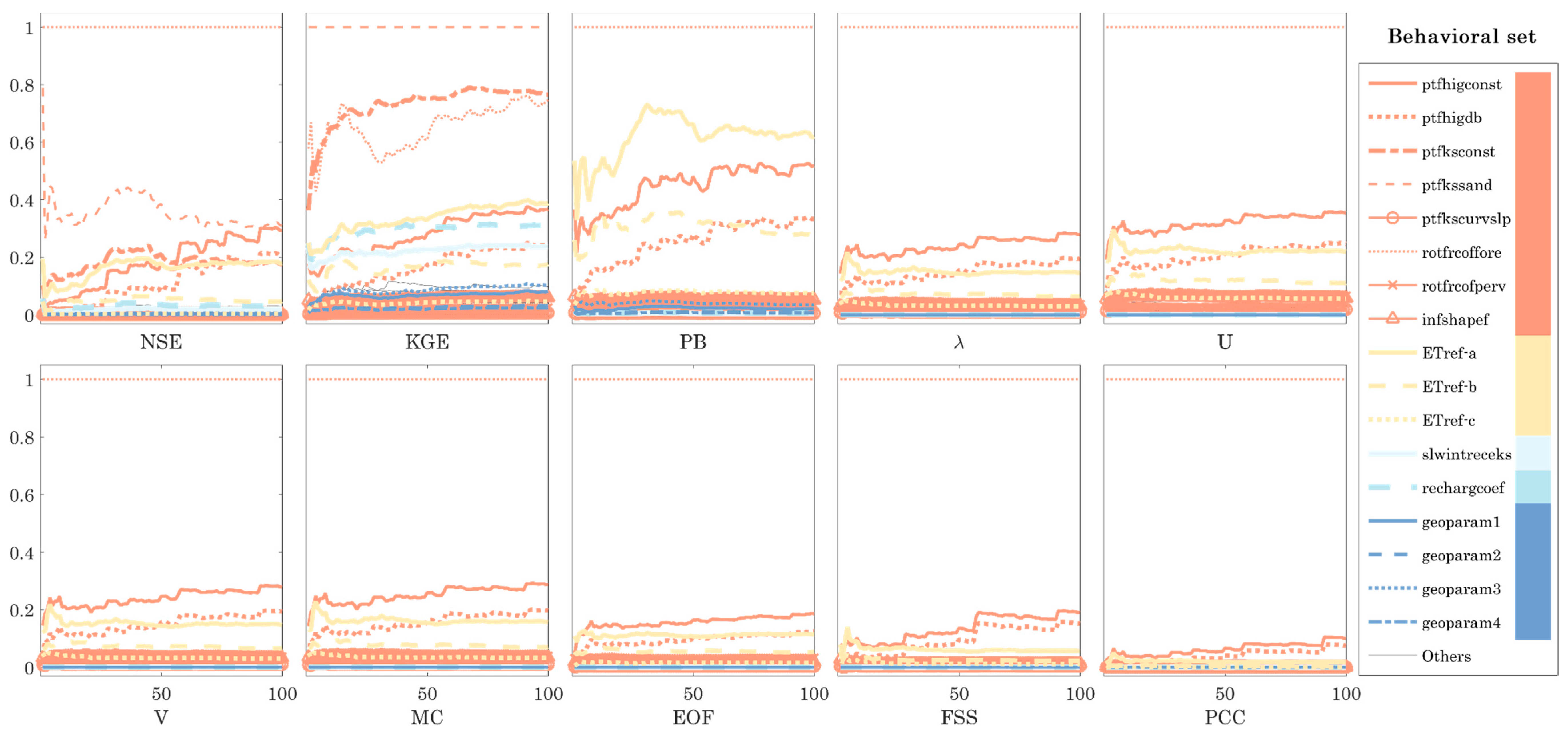
4.2. Latin Hypercube Sampling One-Factor-at-a-Time Sensitivity Analysis
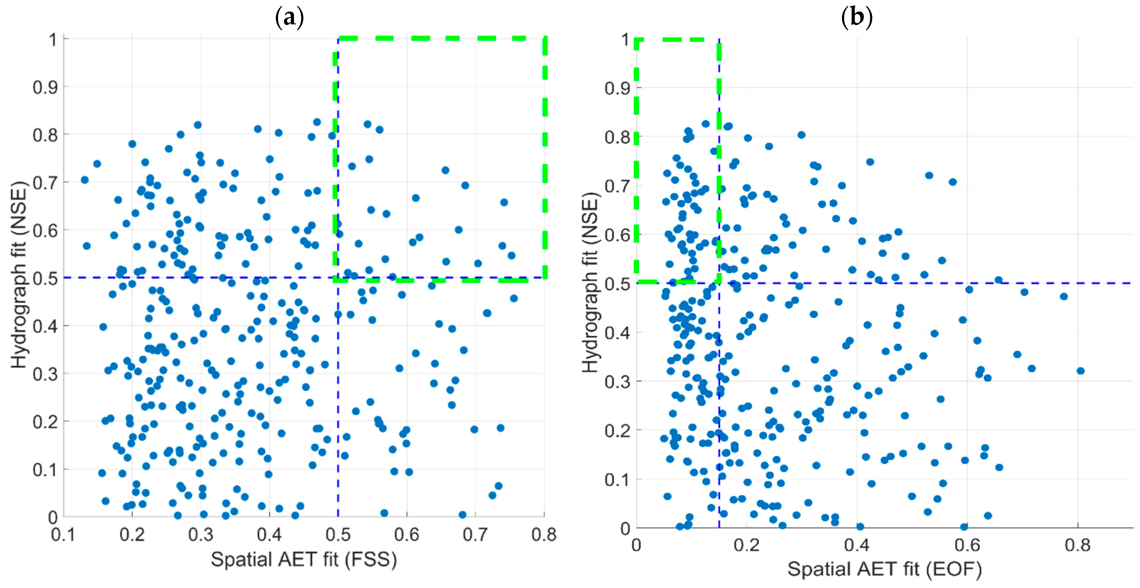
4.3. Random Parameter Sets Based on the 17 Sensitive Parameters Evaluated against NSE and FSS
5. Discussion
Utility of the Multicriteria Spatial Sensitivity Analysis
6. Conclusions
- Based on the detailed analysis of spatial metrics, the EOF, FSS, and Cramér’s V are found to be relevant (nonredundant) pairs for spatial comparison of categorical maps. Further, the PCC metric can provide an easy understanding of map association, although it can be very sensitive to extreme values.
- Based on the results from sensitivity analysis, vegetation and soil parametrization mainly control the spatial pattern of the actual evapotranspiration in the mHM model for this study area.
- Besides, the interception, recharge, and geological parameters are also important for changing streamflow dynamics. Their effect on spatial actual evapotranspiration pattern is substantial but uniform over the basin. For interception, the lacking effect on the spatial pattern of AET is due to the exclusion of rainy days in the spatial pattern evaluation.
- More than half of the 47 parameters included in this study have either little or no effect on simulated spatial patterns, i.e., noninformative parameters, in the Skjern Basin with the chosen setup. In total, only 17 of 47 mHM parameters were selected for a subsequent spatial calibration study.
- The sensitivity maps are consistent with parameter types, as they reflect land cover, LAI, and soil maps of the Skjern Basin.
- Combining NSE with a spatial metric strengthens the physical meaningfulness and robustness of selecting behavioral models.
Author Contributions
Funding
Acknowledgments
Conflicts of Interest
Appendix A

| ID | Parameter | Description | Normalized Sensitivity | |||
|---|---|---|---|---|---|---|
| LHS-OAT Random | LHS-OAT Behavioral | |||||
| KGE | FSS | KGE | FSS | |||
| 1 | ptfhigconst | Constant in pedo-transfer function (ptf) for soils with sand content higher than 66.5% | 0.394 | 0.207 | 0.367 | 0.19 |
| 2 | ptfhigdb | Coefficient for bulk density in pedo-transfer function for soils with sand content higher than 66.5% | 0.261 | 0.17 | 0.243 | 0.151 |
| 3 | ptfksconst | Constant in pedo-transfer function for hydraulic conductivity of soils with sand content higher than 66.5% | 0.366 | 0.003 | 0.765 | 0.005 |
| 4 | ptfkssand | Coefficient for sand content in pedo-transfer function for hydraulic conductivity | 0.469 | 0.005 | 1 | 0.006 |
| 5 | ptfkscurvslp | Exponent in pedo-transfer function for hydraulic conductivity to adjust slope of curve | 0.005 | 0.002 | 0.007 | 0.004 |
| 6 | rotfrcoffore | Root fraction for forested areas | 1 | 1 | 0.746 | 1 |
| 7 | rotfrcofperv | Root fraction for pervious areas | 0.03 | 0.008 | 0.024 | 0.01 |
| 8 | infshapef | Infiltration (inf) shape factor | 0.051 | 0.008 | 0.06 | 0.011 |
| 9 | ETref-a | Intercept | 0.383 | 0.052 | 0.388 | 0.056 |
| 10 | ETref-b | Base coefficient | 0.165 | 0.021 | 0.176 | 0.022 |
| 11 | ETref-c | Exponent coefficient | 0.046 | 0.008 | 0.047 | 0.011 |
| 12 | slwintreceks | Slow (slw) interception | 0.113 | 0 | 0.236 | 0 |
| 13 | rechargcoef | Recharge coefficient (coef) | 0.14 | 0 | 0.309 | 0 |
| 14 | geoparam1 | Parameter for first geological formation | 0.13 | 0 | 0.081 | 0 |
| 15 | geoparam2 | Parameter for second geological formation | 0.045 | 0 | 0.032 | 0 |
| 16 | geoparam3 | Parameter for third geological formation | 0.175 | 0 | 0.105 | 0 |
| 17 | geoparam4 | Parameter for fourth geological formation | 0.038 | 0 | 0.025 | 0 |
References
- Beven, K.; Freer, J. Equifinality, data assimilation, and uncertainty estimation in mechanistic modelling of complex environmental systems using the GLUE methodology. J. Hydrol. 2001, 249, 11–29. [Google Scholar] [CrossRef]
- Demirel, M.C.; Mai, J.; Mendiguren, G.; Koch, J.; Samaniego, L.; Stisen, S. Combining satellite data and appropriate objective functions for improved spatial pattern performance of a distributed hydrologic model. Hydrol. Earth Syst. Sci. 2018, 22, 1299–1315. [Google Scholar] [CrossRef]
- Koch, J.; Demirel, M.C.; Stisen, S. The SPAtial EFficiency metric (SPAEF): Multiple-component evaluation of spatial patterns for optimization of hydrological models. Geosci. Model Dev. 2018, 11, 1873–1886. [Google Scholar] [CrossRef]
- Shin, M.-J.; Guillaume, J.H.A.; Croke, B.F.W.; Jakeman, A.J. Addressing ten questions about conceptual rainfall–runoff models with global sensitivity analyses in R. J. Hydrol. 2013, 503, 135–152. [Google Scholar] [CrossRef]
- Berezowski, T.; Nossent, J.; Chormański, J.; Batelaan, O. Spatial sensitivity analysis of snow cover data in a distributed rainfall-runoff model. Hydrol. Earth Syst. Sci. 2015, 19, 1887–1904. [Google Scholar] [CrossRef]
- Saltelli, A.; Tarantola, S.; Chan, K.P.-S. A Quantitative Model-Independent Method for Global Sensitivity Analysis of Model Output. Technometrics 1999, 41, 39–56. [Google Scholar] [CrossRef]
- Bahremand, A. HESS Opinions: Advocating process modeling and de-emphasizing parameter estimation. Hydrol. Earth Syst. Sci. 2016, 20, 1433–1445. [Google Scholar] [CrossRef]
- Zhuo, L.; Han, D. Could operational hydrological models be made compatible with satellite soil moisture observations? Hydrol. Process. 2016, 30, 1637–1648. [Google Scholar] [CrossRef]
- Rakovec, O.; Hill, M.C.; Clark, M.P.; Weerts, A.H.; Teuling, A.J.; Uijlenhoet, R. Distributed Evaluation of Local Sensitivity Analysis (DELSA), with application to hydrologic models. Water Resour. Res. 2014, 50, 409–426. [Google Scholar] [CrossRef]
- Massmann, C.; Holzmann, H. Analysis of the behavior of a rainfall–runoff model using three global sensitivity analysis methods evaluated at different temporal scales. J. Hydrol. 2012, 475, 97–110. [Google Scholar] [CrossRef]
- Bennett, K.E.; Urrego Blanco, J.R.; Jonko, A.; Bohn, T.J.; Atchley, A.L.; Urban, N.M.; Middleton, R.S. Global Sensitivity of Simulated Water Balance Indicators Under Future Climate Change in the Colorado Basin. Water Resour. Res. 2018, 54, 132–149. [Google Scholar] [CrossRef]
- Lilburne, L.; Tarantola, S. Sensitivity analysis of spatial models. Int. J. Geogr. Inf. Sci. 2009, 23, 151–168. [Google Scholar] [CrossRef]
- Sobol, I. Global sensitivity indices for nonlinear mathematical models and their Monte Carlo estimates. Math. Comput. Simul. 2001, 55, 271–280. [Google Scholar] [CrossRef]
- Cukier, R.I. Study of the sensitivity of coupled reaction systems to uncertainties in rate coefficients. I Theory. J. Chem. Phys. 1973, 59, 3873. [Google Scholar] [CrossRef]
- Morris, M.D. Factorial Sampling Plans for Preliminary Computational Experiments. Technometrics 1991, 33, 161–174. [Google Scholar] [CrossRef]
- Herman, J.D.; Kollat, J.B.; Reed, P.M.; Wagener, T. Technical Note: Method of Morris effectively reduces the computational demands of global sensitivity analysis for distributed watershed models. Hydrol. Earth Syst. Sci. 2013, 17, 2893–2903. [Google Scholar] [CrossRef]
- Razavi, S.; Gupta, H. What Do We Mean by Sensitivity Analysis? The Need for Comprehensive Characterization of ‘Global’ Sensitivity in Earth and Environmental Systems Models. Water Resour. Res. 2015, 51, 3070–3092. [Google Scholar] [CrossRef]
- Cuntz, M.; Mai, J.; Zink, M.; Thober, S.; Kumar, R.; Schäfer, D.; Schrön, M.; Craven, J.; Rakovec, O.; Spieler, D.; et al. Computationally inexpensive identification of noninformative model parameters by sequential screening. Water Resour. Res. 2015, 51, 6417–6441. [Google Scholar] [CrossRef]
- Van Griensven, A.; Meixner, T.; Grunwald, S.; Bishop, T.; Diluzio, M.; Srinivasan, R. A global sensitivity analysis tool for the parameters of multi-variable catchment models. J. Hydrol. 2006, 324, 10–23. [Google Scholar] [CrossRef]
- Stisen, S.; Jensen, K.H.; Sandholt, I.; Grimes, D.I.F.F. A remote sensing driven distributed hydrological model of the Senegal River basin. J. Hydrol. 2008, 354, 131–148. [Google Scholar] [CrossRef]
- Larsen, M.A.D.; Refsgaard, J.C.; Jensen, K.H.; Butts, M.B.; Stisen, S.; Mollerup, M. Calibration of a distributed hydrology and land surface model using energy flux measurements. Agric. For. Meteorol. 2016, 217, 74–88. [Google Scholar] [CrossRef]
- Melsen, L.; Teuling, A.; Torfs, P.; Zappa, M.; Mizukami, N.; Clark, M.; Uijlenhoet, R. Representation of spatial and temporal variability in large-domain hydrological models: Case study for a mesoscale pre-Alpine basin. Hydrol. Earth Syst. Sci. 2016, 20, 2207–2226. [Google Scholar] [CrossRef]
- Koch, J.; Jensen, K.H.; Stisen, S. Toward a true spatial model evaluation in distributed hydrological modeling: Kappa statistics, Fuzzy theory, and EOF-analysis benchmarked by the human perception and evaluated against a modeling case study. Water Resour. Res. 2015, 51, 1225–1246. [Google Scholar] [CrossRef]
- Cornelissen, T.; Diekkrüger, B.; Bogena, H. Using High-Resolution Data to Test Parameter Sensitivity of the Distributed Hydrological Model HydroGeoSphere. Water 2016, 8, 202. [Google Scholar] [CrossRef]
- Cai, G.; Vanderborght, J.; Langensiepen, M.; Schnepf, A.; Hüging, H.; Vereecken, H. Root growth, water uptake, and sap flow of winter wheat in response to different soil water conditions. Hydrol. Earth Syst. Sci. 2018, 22, 2449–2470. [Google Scholar] [CrossRef]
- Wambura, F.J.; Dietrich, O.; Lischeid, G. Improving a distributed hydrological model using evapotranspiration-related boundary conditions as additional constraints in a data-scarce river basin. Hydrol. Process. 2018, 32, 759–775. [Google Scholar] [CrossRef]
- Roberts, N.M.; Lean, H.W. Scale-Selective Verification of Rainfall Accumulations from High-Resolution Forecasts of Convective Events. Mon. Weather Rev. 2008, 136, 78–97. [Google Scholar] [CrossRef]
- Höllering, S.; Wienhöfer, J.; Ihringer, J.; Samaniego, L.; Zehe, E. Regional analysis of parameter sensitivity for simulation of streamflow and hydrological fingerprints. Hydrol. Earth Syst. Sci. 2018, 22, 203–220. [Google Scholar] [CrossRef]
- Westerhoff, R.S. Using uncertainty of Penman and Penman-Monteith methods in combined satellite and ground-based evapotranspiration estimates. Remote Sens. Environ. 2015, 169, 102–112. [Google Scholar] [CrossRef]
- Samaniego, L.; Kumar, R.; Attinger, S. Multiscale parameter regionalization of a grid-based hydrologic model at the mesoscale. Water Resour. Res. 2010, 46. [Google Scholar] [CrossRef]
- Stisen, S.; Sonnenborg, T.O.; Højberg, A.L.; Troldborg, L.; Refsgaard, J.C. Evaluation of Climate Input Biases and Water Balance Issues Using a Coupled Surface–Subsurface Model. Vadose Zone J. 2011, 10, 37–53. [Google Scholar] [CrossRef]
- Jensen, K.H.; Illangasekare, T.H. HOBE: A Hydrological Observatory. Vadose Zone J. 2011, 10, 1–7. [Google Scholar] [CrossRef]
- Mendiguren, G.; Koch, J.; Stisen, S. Spatial pattern evaluation of a calibrated national hydrological model—A remote-sensing-based diagnostic approach. Hydrol. Earth Syst. Sci. 2017, 21, 5987–6005. [Google Scholar] [CrossRef]
- Tucker, C.J. Red and photographic infrared linear combinations for monitoring vegetation. Remote Sens. Environ. 1979, 8, 127–150. [Google Scholar] [CrossRef]
- Jonsson, P.; Eklundh, L. Seasonality extraction by function fitting to time-series of satellite sensor data. IEEE Trans. Geosci. Remote Sens. 2002, 40, 1824–1832. [Google Scholar] [CrossRef]
- Jönsson, P.; Eklundh, L. TIMESAT—A program for analyzing time-series of satellite sensor data. Comput. Geosci. 2004, 30, 833–845. [Google Scholar] [CrossRef]
- Stisen, S.; Højberg, A.L.; Troldborg, L.; Refsgaard, J.C.; Christensen, B.S.B.; Olsen, M.; Henriksen, H.J. On the importance of appropriate precipitation gauge catch correction for hydrological modelling at mid to high latitudes. Hydrol. Earth Syst. Sci. 2012, 16, 4157–4176. [Google Scholar] [CrossRef]
- Refsgaard, J.C.; Stisen, S.; Højberg, A.L.; Olsen, M.; Henriksen, H.J.; Børgesen, C.D.; Vejen, F.; Kern-Hansen, C.; Blicher-Mathiesen, G. Danmarks Og Grønlands Geologiske Undersøgelse Rapport 2011/77; Geological Survey of Danmark and Greenland (GEUS): Copenhagen, Denmark, 2011. [Google Scholar]
- Boegh, E.; Thorsen, M.; Butts, M.; Hansen, S.; Christiansen, J.; Abrahamsen, P.; Hasager, C.; Jensen, N.; van der Keur, P.; Refsgaard, J.; et al. Incorporating remote sensing data in physically based distributed agro-hydrological modelling. J. Hydrol. 2004, 287, 279–299. [Google Scholar] [CrossRef]
- Norman, J.M.; Kustas, W.P.; Humes, K.S. Source approach for estimating soil and vegetation energy fluxes in observations of directional radiometric surface temperature. Agric. For. Meteorol. 1995, 77, 263–293. [Google Scholar] [CrossRef]
- Priestley, C.H.B.; Taylor, R.J. On the Assessment of Surface Heat Flux and Evaporation Using Large-Scale Parameters. Mon. Weather Rev. 1972, 100, 81–92. [Google Scholar] [CrossRef]
- Dee, D.P.; Uppala, S.M.; Simmons, A.J.; Berrisford, P.; Poli, P.; Kobayashi, S.; Andrae, U.; Balmaseda, M.A.; Balsamo, G.; Bauer, P.; et al. The ERA-Interim reanalysis: Configuration and performance of the data assimilation system. Q. J. R. Meteorol. Soc. 2011, 137, 553–597. [Google Scholar] [CrossRef]
- Doherty, J. PEST: Model Independent Parameter Estimation. Fifth Edition of User Manual; Watermark Numerical Computing: Brisbane, Australia, 2005. [Google Scholar]
- McKay, M.D.; Beckman, R.J.; Conover, W.J. A Comparison of Three Methods for Selecting Values of Input Variables in the Analysis of Output from a Computer Code. Technometrics 1979, 21, 239–245. [Google Scholar]
- Du, S.; Wang, L. Aircraft Design Optimization with Uncertainty Based on Fuzzy Clustering Analysis. J. Aerosp. Eng. 2016, 29, 04015032. [Google Scholar] [CrossRef]
- Chu, L. Reliability Based Optimization with Metaheuristic Algorithms and Latin Hypercube Sampling Based Surrogate Models. Appl. Comput. Math. 2015, 4. [Google Scholar] [CrossRef]
- Nash, J.E.; Sutcliffe, J.V. River flow forecasting through conceptual models part I—A discussion of principles. J. Hydrol. 1970, 10, 282–290. [Google Scholar] [CrossRef]
- Gupta, H.V.; Kling, H.; Yilmaz, K.K.; Martinez, G.F. Decomposition of the mean squared error and NSE performance criteria: Implications for improving hydrological modelling. J. Hydrol. 2009, 377, 80–91. [Google Scholar] [CrossRef]
- Goodman, L.A.; Kruskal, W.H. Measures of Association for Cross Classifications*. J. Am. Stat. Assoc. 1954, 49, 732–764. [Google Scholar] [CrossRef]
- Finn, J.T. Use of the average mutual information index in evaluating classification error and consistency. Int. J. Geogr. Inf. Syst. 1993, 7, 349–366. [Google Scholar] [CrossRef]
- Cramér, H. Mathematical Methods of Statistics; Princeton University Press: Princeton, NJ, USA, 1946; ISBN 0-691-08004-6. [Google Scholar]
- Hargrove, W.W.; Hoffman, F.M.; Hessburg, P.F. Mapcurves: A quantitative method for comparing categorical maps. J. Geogr. Syst. 2006, 8, 187–208. [Google Scholar] [CrossRef]
- Pearson, K. Notes on the History of Correlation. Biometrika 1920, 13. [Google Scholar] [CrossRef]
- Speich, M.J.R.; Bernhard, L.; Teuling, A.J.; Zappa, M. Application of bivariate mapping for hydrological classification and analysis of temporal change and scale effects in Switzerland. J. Hydrol. 2015, 523, 804–821. [Google Scholar] [CrossRef]
- Rees, W.G. Comparing the spatial content of thematic maps. Int. J. Remote Sens. 2008, 29, 3833–3844. [Google Scholar] [CrossRef]
- Perry, M.A.; Niemann, J.D. Analysis and estimation of soil moisture at the catchment scale using EOFs. J. Hydrol. 2007, 334, 388–404. [Google Scholar] [CrossRef]
- Mascaro, G.; Vivoni, E.R.; Méndez-Barroso, L.A. Hyperresolution hydrologic modeling in a regional watershed and its interpretation using empirical orthogonal functions. Adv. Water Resour. 2015, 83, 190–206. [Google Scholar] [CrossRef]
- Gilleland, E.; Ahijevych, D.; Brown, B.G.; Casati, B.; Ebert, E.E. Intercomparison of Spatial Forecast Verification Methods. Weather Forecast. 2009, 24, 1416–1430. [Google Scholar] [CrossRef]
- Wolff, J.K.; Harrold, M.; Fowler, T.; Gotway, J.H.; Nance, L.; Brown, B.G. Beyond the Basics: Evaluating Model-Based Precipitation Forecasts Using Traditional, Spatial, and Object-Based Methods. Weather Forecast. 2014, 29, 1451–1472. [Google Scholar] [CrossRef]
- Koch, J.; Mendiguren, G.; Mariethoz, G.; Stisen, S. Spatial Sensitivity Analysis of Simulated Land Surface Patterns in a Catchment Model Using a Set of Innovative Spatial Performance Metrics. J. Hydrometeorol. 2017, 18, 1121–1142. [Google Scholar] [CrossRef]
- Montanari, A. Large sample behaviors of the generalized likelihood uncertainty estimation (GLUE) in assessing the uncertainty of rainfall-runoff simulations. Water Resour. Res. 2005, 41. [Google Scholar] [CrossRef]
- Demirel, M.C.; Booij, M.J.; Hoekstra, A.Y. Effect of different uncertainty sources on the skill of 10 day ensemble low flow forecasts for two hydrological models. Water Resour. Res. 2013, 49, 4035–4053. [Google Scholar] [CrossRef]
- Li, J.; Duan, Q.Y.; Gong, W.; Ye, A.; Dai, Y.; Miao, C.; Di, Z.; Tong, C.; Sun, Y. Assessing parameter importance of the Common Land Model based on qualitative and quantitative sensitivity analysis. Hydrol. Earth Syst. Sci. 2013, 17, 3279–3293. [Google Scholar] [CrossRef]
- Gan, Y.; Duan, Q.; Gong, W.; Tong, C.; Sun, Y.; Chu, W.; Ye, A.; Miao, C.; Di, Z. A comprehensive evaluation of various sensitivity analysis methods: A case study with a hydrological model. Environ. Model. Softw. 2014, 51, 269–285. [Google Scholar] [CrossRef]


| Variable | Description | Period | Spatial Resolution | Remark | Source |
|---|---|---|---|---|---|
| LAI | Fully distributed 8-day time varying LAI dataset | 1990–2014 | 1 km | 8 day to daily | MODIS and Mendiguren et al. [33] |
| AET | Actual evapotranspiration | 1990–2014 | 1 km | daily | MODIS, TSEB |
| Parameter | Unit | Description | Initial Value ** | Lower Bound | Upper Bound |
|---|---|---|---|---|---|
| ETref-a | - | Intercept | 0.95 | 0.5 | 1.2 |
| ETref-b | - | Base Coefficient | 0.2 | 0 | 1 |
| ETref-c | - | Exponent Coefficient | −0.7 | −2 | 0 |
| Description | Best Value | Abbreviation | Group | Reference |
|---|---|---|---|---|
| Nash–Sutcliffe Efficiency | 1.0 | NSE | Streamflow | [47] |
| Kling–Gupta Efficiency | 1.0 | KGE | Streamflow | [48] |
| Percent Bias | 0.0 | PB | Streamflow | |
| Goodman and Kruskal’s Lambda | 1.0 | λ | Spatial pattern | [49] |
| Theil’s Uncertainty coefficient | 1.0 | U | Spatial pattern | [50] |
| Cramér’s V | 1.0 | V | Spatial pattern | [51] |
| Map Curves | 1.0 | MC | Spatial pattern | [52] |
| Empirical Orthogonal Function | 0.0 | EOF | Spatial pattern | [23] |
| Fraction Skill Score | 1.0 | FSS | Spatial pattern | [27] |
| Pearson Correlation Coefficient | 1.0 | PCC | Spatial pattern | [53] |
| MAP_ID | λ | U | V | MC | EOF * | FSS | PCC | Survey Similarity |
|---|---|---|---|---|---|---|---|---|
| 1 | 0.68 | 0.59 | 0.81 | 0.76 | 0.02 | 0.96 | 0.95 | 0.86 |
| 6 | 0.49 | 0.50 | 0.73 | 0.72 | 0.05 | 0.97 | 0.86 | 0.75 |
| 8 | 0.28 | 0.30 | 0.57 | 0.53 | 0.06 | 0.96 | 0.86 | 0.64 |
| 12 | 0.39 | 0.37 | 0.63 | 0.59 | 0.06 | 0.89 | 0.86 | 0.61 |
| 5 | 0.50 | 0.44 | 0.70 | 0.65 | 0.05 | 0.91 | 0.87 | 0.59 |
| 2 | 0.20 | 0.26 | 0.52 | 0.50 | 0.08 | 0.89 | 0.79 | 0.59 |
| 10 | 1.0 | 1.0 | 1.0 | 1.0 | 0.0 | 1.0 | 1.0 | 0.57 |
| 11 | 0.00 | 0.04 | 0.20 | 0.32 | 0.21 | 0.87 | 0.37 | 0.42 |
| 4 | 0.00 | 0.07 | 0.26 | 0.35 | 0.25 | 0.77 | 0.27 | 0.36 |
| 3 | 0.00 | 0.17 | 0.39 | 0.40 | 0.15 | 0.93 | 0.70 | 0.29 |
| 9 | 0.20 | 0.21 | 0.48 | 0.47 | 0.16 | 0.87 | 0.48 | 0.23 |
| 7 | 0.00 | 0.00 | 0.04 | 0.29 | 0.28 | 0.73 | −0.01 | 0.10 |
| R2 Score | λ | U | V | MC | EOF | FSS | PCC | Survey Similarity |
|---|---|---|---|---|---|---|---|---|
| λ | 1 | 0.97 | 0.88 | 0.97 | 0.71 | 0.51 | 0.59 | 0.46 |
| U | 1 | 0.90 | 0.99 | 0.72 | 0.59 | 0.63 | 0.41 | |
| V | 1 | 0.93 | 0.90 | 0.72 | 0.85 | 0.59 | ||
| MC | 1 | 0.77 | 0.61 | 0.67 | 0.49 | |||
| EOF | 1 | 0.79 | 0.96 | 0.72 | ||||
| FSS | 1 | 0.84 | 0.52 | |||||
| PCC | 1 | 0.69 | ||||||
| Survey Similarity | 1 | |||||||
© 2018 by the authors. Licensee MDPI, Basel, Switzerland. This article is an open access article distributed under the terms and conditions of the Creative Commons Attribution (CC BY) license (http://creativecommons.org/licenses/by/4.0/).
Share and Cite
Demirel, M.C.; Koch, J.; Mendiguren, G.; Stisen, S. Spatial Pattern Oriented Multicriteria Sensitivity Analysis of a Distributed Hydrologic Model. Water 2018, 10, 1188. https://doi.org/10.3390/w10091188
Demirel MC, Koch J, Mendiguren G, Stisen S. Spatial Pattern Oriented Multicriteria Sensitivity Analysis of a Distributed Hydrologic Model. Water. 2018; 10(9):1188. https://doi.org/10.3390/w10091188
Chicago/Turabian StyleDemirel, Mehmet Cüneyd, Julian Koch, Gorka Mendiguren, and Simon Stisen. 2018. "Spatial Pattern Oriented Multicriteria Sensitivity Analysis of a Distributed Hydrologic Model" Water 10, no. 9: 1188. https://doi.org/10.3390/w10091188
APA StyleDemirel, M. C., Koch, J., Mendiguren, G., & Stisen, S. (2018). Spatial Pattern Oriented Multicriteria Sensitivity Analysis of a Distributed Hydrologic Model. Water, 10(9), 1188. https://doi.org/10.3390/w10091188