Article

Multiple Linear Regression Models for Predicting Nonpoint-Source Pollutant Discharge from a Highland Agricultural Region

1
Department of Biosystems and Convergence Engineering, Catholic Kwandong University, 24 Beomil-ro, 579 beon-gil, Gangneung-si, Gangwon-do 25601, Korea
2
Department of Urban Planning and Real Estate, Cheongju University, 298 Daeseongro, Cheongwon-gu, Cheongju, Chungbuk 28503, Korea
*
Author to whom correspondence should be addressed.
Water 2018, 10(9), 1156; https://doi.org/10.3390/w10091156
Submission received: 25 July 2018 / Revised: 26 August 2018 / Accepted: 27 August 2018 / Published: 29 August 2018

Abstract

:
Sediment runoff from dense highland field areas greatly affects the quality of downstream lakes and drinking water sources. In this study, multiple linear regression (MLR) models were built to predict diffuse pollutant discharge using the environmental parameters of a basin. Explanatory variables that influence the sediment and pollutant discharge can be identified with the model, and such research could play an important role in limiting sediment erosion in the dense highland field area. Pollutant load per event, event mean concentration (EMC), and pollutant load per area were estimated from stormwater survey data from the Lake Soyang basin. During the wet season, heavy rains cause large amounts of suspended sediment and the occurrence of such rains is increasing due to climate change. The explanatory variables used in the MLR models are the percentage of fields, subbasin area, and mean slope of subbasin as topographic parameters, and the number of preceding dry days, rainfall intensity, rainfall depth, and rainfall duration as rainfall parameters. In the MLR modeling process, four types of regression equations with and without log transformation of the explanatory and response variables were examined to identify the best performing regression model. The performance of the MLR models was evaluated using the coefficient of determination (R2), root mean square error (RMSE), coefficient of variation of the root mean square error (CV(RMSE)), the ratio of the RMSE to the standard deviation of the observed data (RSR) and the Nash–Sutcliffe model efficiency (NSE). The performance of the MLR models of pollutant load except total nitrogen (TN) was good under the condition of RSR, and satisfactory for the NSE and R2. In the EMC and load/area models, the performance for suspended solids (SS) and total phosphorus (TP) was good for the RSR, and satisfactory for the NSE and R2. The standardized coefficients for the models were analyzed to identify the influential explanatory variables in the models. In the final performance evaluation, the results of jackknife validation indicate that the MLR models are robust.

Graphical Abstract

1. Introduction

In Lake Soyang basin of South Korea, large amounts of sediment are discharged from highland agricultural field regions in the wet season. To develop environmental preservation measures that protect water resources from the turbid water problem and diffuse pollution, prediction models are necessary to estimate the amount of pollutants discharged from subbasins. In this study, a multiple linear regression (MLR) model is established to predict the pollutant runoff discharge using environmental parameters, such as land use, rainfall, and topography.
In South Korea, rainfall events of 200 mm or more occurred only once annually, on average, until the end of the 1970s, but increased to a frequency of two per year in the 1980s and thereafter occurred five times in both 1984 and 1998. And, annual precipitation increased by 19% in the past decade, compared to the first half of the 20th century [1]. Conditions in Lake Soyang, located in the upper reaches of the Han River, greatly affect the water quality of the water supply of the capital region of South Korea. Discharged sediments from the highland field area flow into Lake Soyang in the wet season. Consequently, the turbidity of the lake increases to high levels and persists for a long time. In July 2006, a heavy rain event occurred in the Lake Soyang watershed. Overall, 670 mm fell over 8 days, with a maximum intensity of 66 mm per hour. The suspended sediment stayed in Lake Soyang for an extended period of time because of stratification; thus, the turbidity of the lake remained high and was measured at over 20 nephelometric turbidity units (NTU) for 168 days [2,3].
Regression models have been developed to estimate the sediment discharge using the subbasin environmental parameters in many areas. Valtanen et al. [4] applied stepwise multiple linear regression (SMLR) analysis to identify the variables that best explained the variation in event mass loads (EMLs) in each study catchment during cold and warm periods. Runoff duration, peak flow, antecedent dry period, mean runoff intensity, total suspended solids (TSS), TN, TP and total organic carbon (TOC) were used as explanatory variables. Another SMLR analysis was also carried out to assess whether catchment variables explain the EML and EMC values during the cold and warm periods [4]. The catchment variables included total impervious area and land use type. All data were log10-transformed to obtain approximately normal distributions. Bian et al. [5] proposed a procedure combining different statistical methods and a hydrological model to quantify the annual runoff response to spatial and temporal variations in impervious surface areas in an urbanized basin. A hydrological model relating annual runoff depth to precipitation, potential evapotranspiration and spatial metrics of the impervious area for baseline periods and periods of change was built using stepwise multiple regression analysis. Roman et al. [6] developed multivariate regression models to enable the prediction of mean annual suspended sediment discharge on the basis of basin characteristics, which is useful for many ungaged river locations in the eastern United States. The models are based on long-term mean sediment discharge estimates and explanatory variables, such as drainage area, mean elevation, and urban area, obtained from a combined dataset of 1201 US Geological Survey (USGS) stations. Tuset et al. [7] analyzed rainfall, runoff and sediment transport relationships in a meso-scale Mediterranean mountain catchment. The relationships among rainfall, runoff and suspended sediment transport were analyzed with Pearson correlations and multivariate regression analysis. The multivariate regression method was used to analyze the relationship between the independent variables (pre-event conditions, rainfall and runoff) and suspended sediment transport for all flood events. Seasonal relationships between total surface runoff and total sediment transport indicate that the sediment transport magnitude shows a clear seasonality influenced by rainfall intensity and sediment availability.
Buendia et al. [8] attempted to use empirical relationships to assess the relationship between sediment yield and basin scale and to provide an update on the main drivers controlling sediment yield in these particular river systems. Quantile regression analysis was used to assess the correlation between basin area and sediment yield, while additional basin-scale descriptors were related to sediment yield by means of multiple regression analysis. The performance of the model was tested through the jackknife validation method [8,9,10,11,12,13,14]. Paule-Mercado et al. [15] used MLRs to identify the significant parameters affecting fecal-indicator bacteria concentrations and to predict the response of bacteria concentrations to changes in land use and land cover. Stormwater temperature, 5-day biochemical oxygen demand (BOD5), turbidity, TSS, and antecedent dry days were the most influential independent variables for the bacteria concentrations at the monitoring sites. Several studies have utilized linear regression techniques to predict bacteria concentrations in rivers [16,17,18,19]. Furthermore, regression models have been widely used to predict and characterize rainfall and runoff characteristics and to determine the relationship between these two variables [20,21,22,23,24,25,26]. Process-based erosion prediction models have also been established to predict the intensity of soil erosion in a particular area [27,28,29,30].
In this study area, two types of environmental parameters affect the stormwater sediment runoff: meteorological factors, such as rainfall depth, rainfall intensity, rainfall duration; and number of preceding dry days and topographic factors, such as percentage of upland field area, subbasin area, and subbasin slope. In this study, the Pearson correlation test was employed to identify the linear relationship between the explanatory environmental parameters and the observed stormwater discharge. SMLR analysis was applied to identify the best performing regression model. Four types of regression equations were examined to determine the best MLR model. Explanatory and dependent variables with and without log e-transformation were tested. Then, the MLR models were validated via a jackknife validation procedure.

2. Materials and Methods

2.1. Study Area and Field Data

Lake Soyang formed following the construction of the Soyang River Dam. The dam was built to provide irrigation water, flood control and hydroelectric power. The dam has a height of 123 m, a length of 530 m, and a total storage capacity of 2900 million m3. The basin area is 2969.3 km2; the forest occupies 86.4%; and the dry field, paddy field and residential areas occupy 4.4%, 1.58%, and 1.60% of the basin, respectively.
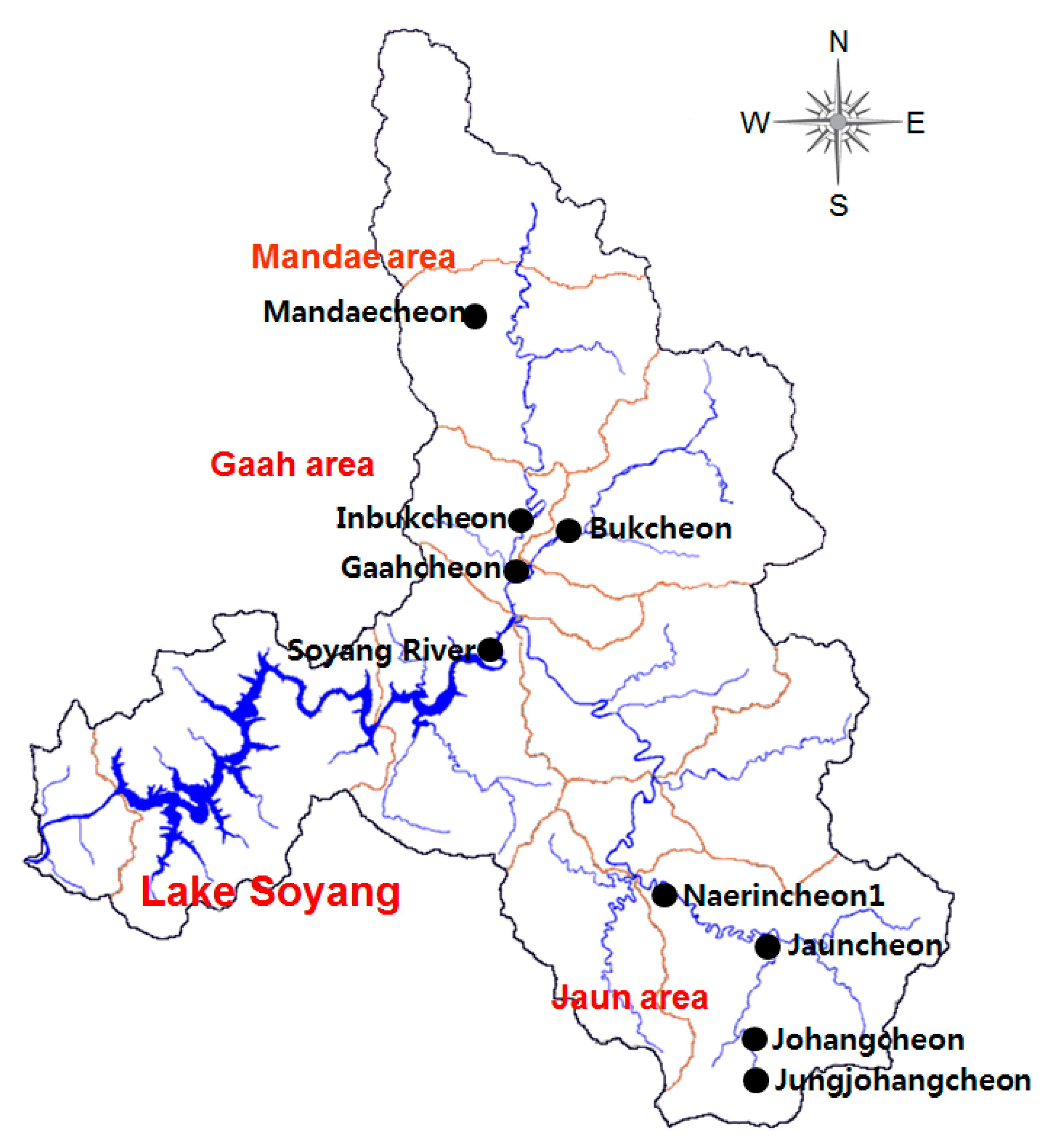
In Lake Soyang basin (Figure 1), sediment discharge occurred mainly from the upper part of the basin. Land use in the tributary watersheds in the dense highland upland field area is shown in Table 1. In the case of Mandaecheon, the percentage of agricultural area is 27.7%, and upland fields represent 75% of the agricultural land. The Jungjohangcheon, Johangcheon and Jauncheon subbasins contain very small paddy field areas. In the highland area, to decrease the damage caused by the continuous cultivation of economic crops, manage pests, maximize crop productivity and improve soil fertility, 30–50 cm of soil dressing has been applied to the top layer of soil. This soil dressing is a significant contributor to the sediment discharge from the highland fields.
During rainfall, water sampling and flow measurements were performed at the same time. Field surveys were conducted to perform flow measurements at most of the survey points. For the remaining points, such as Inbukcheon, Bukcheon, and Soyang River, real-time water level and flow measurements were obtained from the Ministry of Land Infrastructure and Transport and the Korea Water Resources Corporation. The sampled water from the measurement sites was delivered to the laboratory as quickly as possible, and BOD, chemical oxygen demand (COD), SS, TP, TN, and TOC were analyzed using standard methods [2].
In the statistical analysis of this study, the results of stormwater runoff surveys from 2013 to 2016 at nine points in the Jaun, Mandae and Gaha area [31] were used. Of the 79 rainfall events, nine data were too high or too low for rainfall amount due to runoff load measurements and calculation errors; those data were excluded. The discharge load survey was performed from the beginning of the rainfall to the point where it returned to the normal water level after the end of the rainfall. Runoff discharge data of 70 storm events were used to build the MLR models to predict the pollutant load, EMC and pollutant load per area. The range of the rainfall depth used in the MLR model construction was from 10 mm to 215 mm.

2.2. Data Analysis

Using water quality and runoff flow data from 70 rainfall events in the Lake Soyang basin, pollutant load per event, EMC, and pollutant load per area were estimated for each rainfall event. The total pollutant load during a rainfall event was calculated using Equation (1). The EMC was defined as the pollutant mass contained in the runoff event divided by the total flow volume of the event. The total pollutant load was divided by the subbasin area to estimate the pollutant load per area.
  T o t a l   p o l l u t i o n   l o a d / r a i n f a l l   e v e n t = i = 1   n   C i Q i Δ t i
  E M C = Q i C i Δ t   Q i Δ t
where n represents the number of total measurements, Qi is the runoff flow at n number of time steps (∆t) and Ci is the concentration of a water quality measurement.
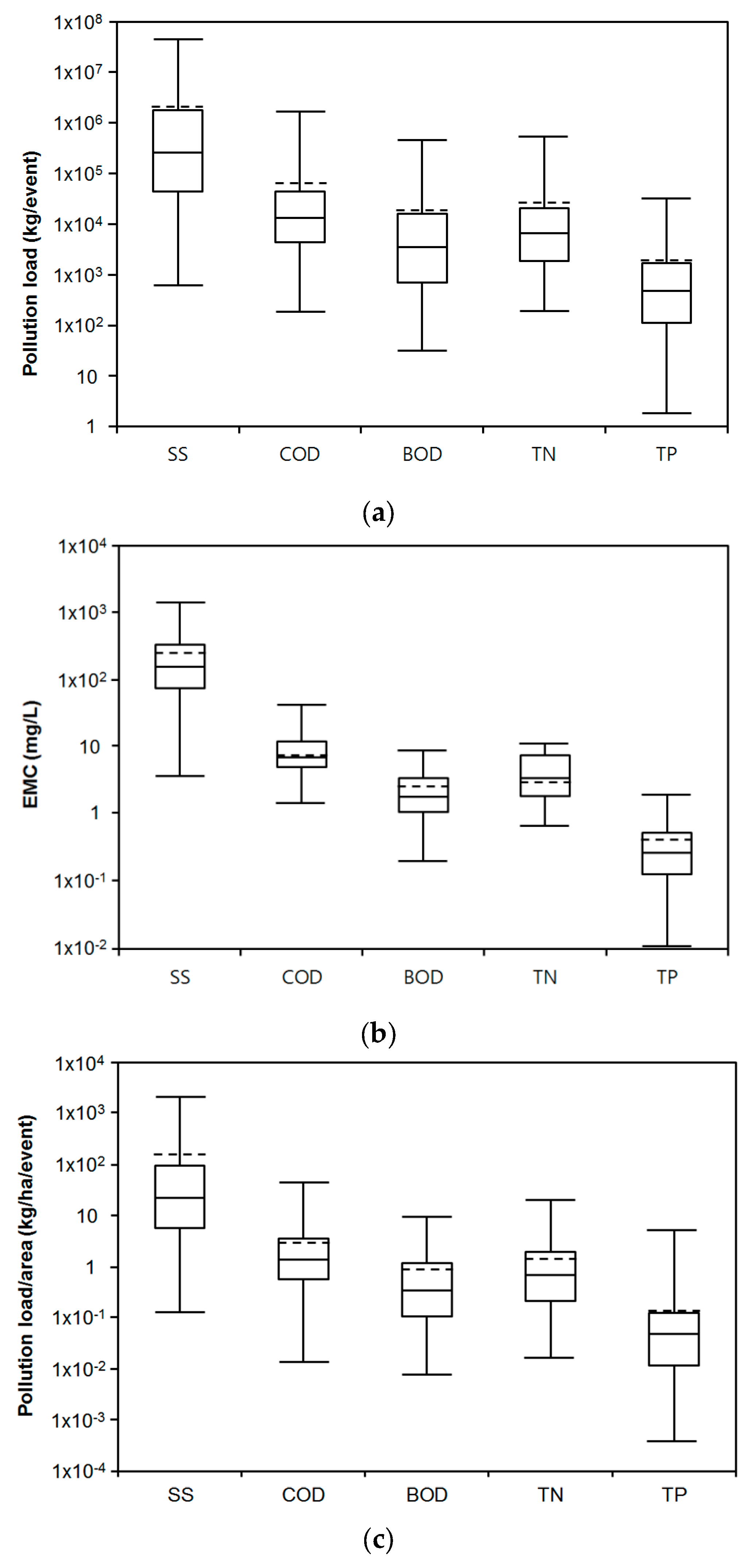
The distribution of the nonpoint pollutant discharge for the 70 rainfall events from 2013 to 2016 is presented in Table 2. Figure 2 shows box plots of pollutant load per event, EMC, and pollutant load per area at the survey points in the Lake Soyang basin. The maximum, minimum and median values of the suspended sediment (SS) load/event were 46,125,100 kg, 613 kg and 263,083 kg, respectively. The maximum, minimum and median values of the TP load/event were 32,406 kg, 1.83 kg and 480 kg, respectively. As shown in Figure 2, all the mean values of the pollutant loads are larger than the values of the third quartile, and the distributions are biased toward the high values. The maximum, minimum and median values of the SS EMC were 1437 mg/L, 3.8 mg/L and 157 mg/L, respectively. The maximum, minimum and median values of the TP EMC were 1.96 mg/L, 0.011 mg/L and 0.27 mg/L, respectively. All the mean values of the EMCs lie between the 50th percentile and the 75th percentile, and the distributions are relatively uniform.
The explanatory variables that are considered to explain the nonpoint pollutant discharge in the MLR models are the percentage of fields (% field), subbasin area (SA), and mean slope of subbasin (slope) as topographic parameters, and the number of preceding dry days (Ndry), rainfall intensity (Rint), rainfall depth (Rain), and rainfall duration (Dur) as rainfall parameters (Table 3).
A Pearson correlation coefficient matrix was used to identify the correlations among the surveyed pollutant discharge estimates and the explanatory variables. The correlations among natural log-transformed variables were also tested using Pearson correlation.

2.3. MLR Model Building

MLR modeling was performed to predict the pollutant discharge from the subbasins in the Soyang River. The models were built to explain the pollutant discharge using the subbasin topographic and rainfall data. In the MLR modeling, four types of regression equations are examined:
Type 1 : Y = a 0 + i = 1   n a i X i
Type 2 : L n ( Y )   = a 0 + i = 1 n a i X i
Type 3 : Y = e a 0 X 1 a 1 X 2 a 2 X n a n   o r   L n ( Y )   = a 0 + i = 1 n ( a i L n ( X i ) )
Type 4 : Y = e a 0 X 1 a 1 X 2 a 2 X m a m e a m + 1 X m + 1 e a n X n   o r   L n ( Y )   = a 0 + i = 1 m ( a i L n ( X i ) ) + i = m + 1 n ( a i X i )
where a0 is the regression constant and ai is the regression coefficient of the explanatory variable Xi. In type 1, the original variables are used to build the MLR model. In type 2, dependent variables, such as pollutant load, EMC and load/area, are log e-transformed to reduce skewness. In type 3, all the explanatory and dependent variables are log e-transformed. In type 4, the dependent variables and some of the explanatory variables are log e-transformed. The fitness of the four regression equations was evaluated by the coefficients of determination of the MLR models. The MLR models were examined in terms of their ability to predict the runoff pollutant discharge for each water quality variable (SS, COD, BOD, TN, and TP).
Collinearity may introduce serious stability problems, such as high mean square errors, in a regression model. Therefore, the collinearity of the predictor variables in the created MLR model were tested by calculating the variance inflation factor (VIF) [32]. Collinearity is present when the largest VIF is greater than 10 or the average VIF value is substantially greater than 1 [32,33]. VIFs were calculated to analyze the multicollinearity in this MLR model.
The MLR model performance was evaluated using the R2, RMSE, CV(RMSE), RSR and the NSE.
  R 2 = [ i = 1   n ( P i P ¯ ) ( O i O ¯ ) ] 2 i = 1 n ( P i P ¯ ) 2 i = 1 n ( O i O ¯ ) 2
  R M S E = [ 1 N i = 1   n ( P i O i ) 2 ] 1 / 2
  C V ( R M S E   ) = [ j = 1 n ( P i j O i j ) 2 / n ] 1 / 2 ( i = 1 n O i j / n )
  R S R = [ i = 1   n ( O i P i ) 2 ] [ i = 1 n ( O i O ¯ ) 2 ]
  N S E = 1 i = 1   n ( O i P i ) 2 i = 1 n ( O i O ¯ ) 2
where Oi is the observed daily load, O ¯ is the mean of the observed daily load, pi is the calculated daily load, and n is the number of data values. The R2 index describes the ability of the model to explain variability among the data. RSR incorporates the benefits of error index statistics and includes a scaling/normalization factor; the lower the RSR is, the better the model simulation performance. The performance ratings for stream flow proposed by Moriasi et al. [33] were ‘very good’ (0.00 ≤ RSR ≤ 0.50), ‘good’ (0.50 < RSR ≤ 0.60), or ‘satisfactory’ (0.60 < RSR ≤ 0.70). NSE is a normalized statistic that reflects the relative magnitude of the residual variance compared with the variance in the observed data (good (NSE > 0.7), satisfactory (0.4 < NSE ≤ 0.7) and unsatisfactory (NSE ≤ 0.4)) [30,34].
Finally, the performance of the MLR model was tested using the jackknife validation method [8,11,14]. This method consists of deleting one site and carrying out the multiple regression analysis with the same dependent variables and the remaining sites. The pollutant discharge of the deleted site is calculated with the equation resulting from the multiple regression associated with the remaining sites. This process is repeated, deleting one site each time.

3. Results and Discussion

3.1. Correlation Analysis between Nonpoint Pollutant Discharge and Explanatory Variables

Table 4 shows the Pearson correlation between runoff discharge and subbasin characteristics, without log transformation of the variables. In Table 5, the Pearson correlation matrix between log-transformed variables is introduced. As the values of the correlation coefficients between log-transformed variables were slightly higher (r < 0.69; Table 5) than those of the non-log-transformed variables (r < 0.65; Table 4), we used log-transformed variables as explanatory variables in the MLR models. Compared to other environmental parameters, the rainfall depth and subbasin area showed a relatively significant correlation with most response discharge variables. The rainfall intensity had a relatively significant positive correlation with the response variables of EMC and load/area because the rainfall intensity directly affects the EMC and load/area of each storm event. On the other hand, the subbasin slope had a negative correlation with the response variables of EMC and load/area.

3.2. MLR Analysis

Four types of MLR models corresponding to Equations (3)–(6) were tested to identify the most suitable models (Table 6). The R2 values for SS, COD, BOD, TN, and TP in the type 1 MLR of pollutant load ranged from 0.275 to 0.447. The R2 values for SS, COD, BOD, TN, and TP in the type 1 MLR of EMC and load/area were also low, indicating poor performance of the regression models. The R2 values for SS, COD, BOD, TN, and TP in the type 2 MLR of pollutant load were 0.76, 0.67, 0.64, 0.65, and 0.80, respectively. The R2 values of the type 2 MLR were quite high, but most of the VIF values were larger than 5, with a few values greater than 10. Thus, the VIF showed that multicollinearity was observed in the established models and that the type 2 MLR was not adapted. Although the R2 values of the type 2 MLR for load/area were acceptable, the VIF values were high, indicating multicolinearity. VIF values and other statistics of MLRs were presented only for the selected model. The results of the MLR model employing the type 4 equation are listed in Table 7, Table 8 and Table 9.
The R2 values for SS, COD, BOD, TN, and TP in the type 3 MLR of the pollutant load were also fairly high, but all VIF values were less than 5. Among the type 3 MLR models, the SS, TN, and TP in the MLR of EMC and the SS and TP in the MLR of load/area showed acceptable R2 values. The values of R2 for SS, COD, BOD, TN, and TP in the type 4 MLR of pollutant load were 0.74, 0.69, 0.69, 0.61, and 0.74 respectively. The R2 values of the type 4 MLR were a little better than those of the type 3 MLR, and all VIF values were less than 5. Thus, we selected the type 4 equation as the MLR model to predict the runoff pollutant discharge in the study area. However, the COD and BOD in the MLR of EMC and COD and TN in the MLR of load/area could not explain the variance in the pollutant discharge properly.
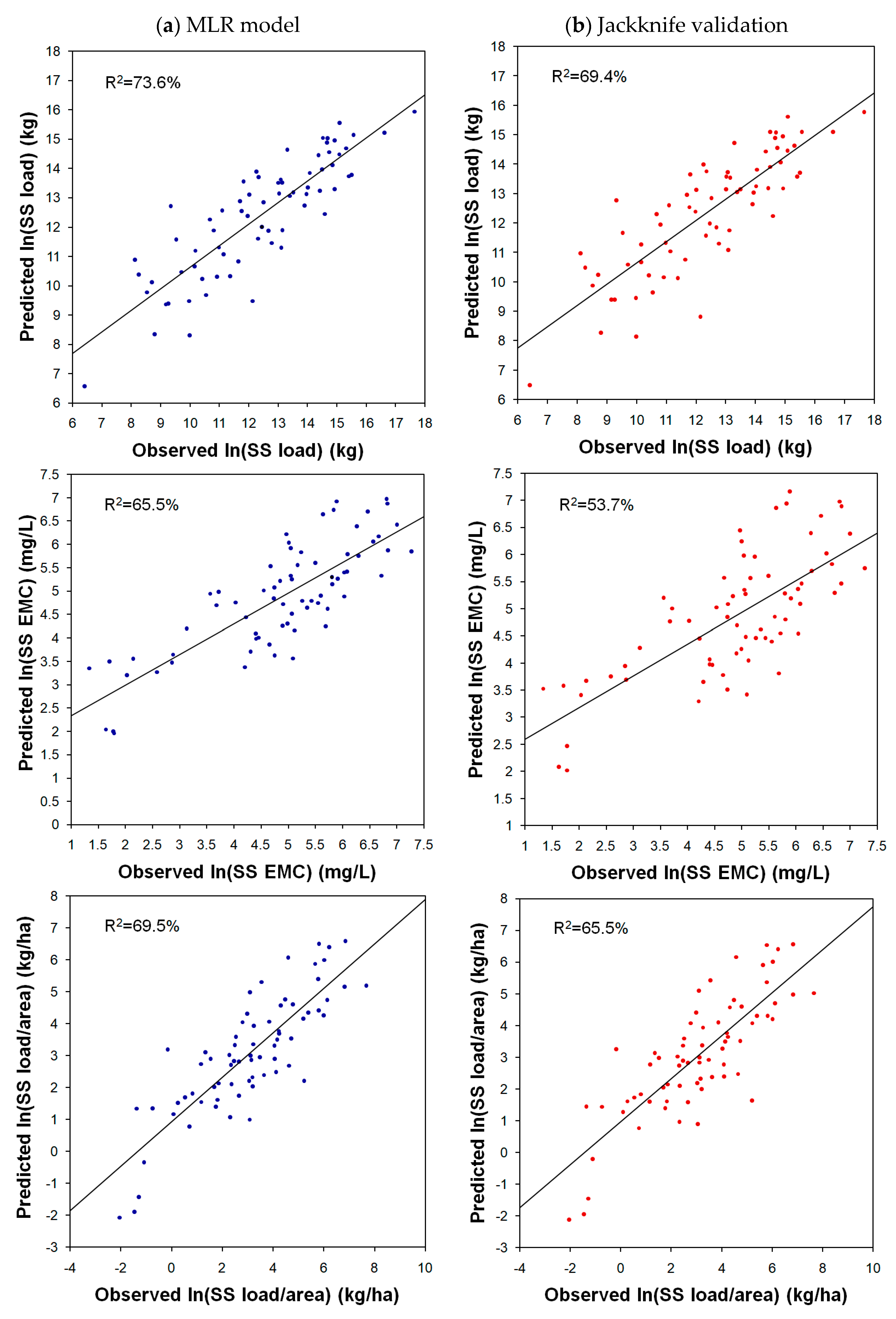
Using the stepwise variable selection method, two to five variables were retained in the pollutant load model, as shown in Table 7. In the case of the SS model, given the R2 value, 73.6% of the variability of the dependent variable ln(SS load) is explained by the four explanatory variables. The MLR models indicated in Table 7, Table 8 and Table 9 are statistically significant at p < 0.0001 except for the ln(COD EMC) model (p = 0.00019). The R2 values for SS, COD, BOD, TN, and TP in the type 4 MLR of pollutant load were fairly high (0.614 < R2 < 0.741), as indicated in Table 7. The performance evaluation by CV(RMSE) [35] shows that the SS model was the best and that the other models of the water quality variables were also acceptable. The range of RSR for SS, COD, BOD, and TP in the MLR models of pollutant load (Table 7) was from 0.509 to 0.559, and the performance of the MLR for these variables was good [34]. The RSR for TN was 0.622, and the performance of the TN model was satisfactory. The NSE values for the MLR models of pollutant load ranged from 0.61 to 0.74, and the MLR models of the pollutant load had good performance. As a special case, in linear regression forecasting models like this study, NSE is equal to the coefficient of determination, R2 [36]. Overall, all the MLR models of the pollutant load had good prediction performance.
All VIF values in Table 7 are lower than 5, and the mean VIF values are not large. These results suggest that the coefficient of regression for the explanatory variables could be statistically acceptable and that multicollinearity was not present in the established models.
Standardized coefficients refer to how many standard deviations a dependent variable will change in response to an increase of one standard deviation in the predictor variable. This statistic allows us to compare the relative contribution of each independent variable in the prediction of the dependent variable. The higher the absolute value of a coefficient is, the more important the weight of the corresponding variable. Standardized coefficients are useful for comparing effects across different measures. The standardized regression coefficients of Table 7 indicate that subbasin area (0.576 < βi < 0.709) and rainfall depth (0.453 < βi < 0.563) are important influential parameters for all the load predictions. In addition, % field has relatively small effects on the SS, BOD and TP models.
The area with the high density of highland fields in Lake Soyang basin has steeper slopes than the other areas. However, Lake Soyang basin also contains highly mountainous terrain; thus, the mean slopes of the dense highland field subbasins are lower than the average slope of the entire Lake Soyang basin. Therefore, the standardized regression coefficients of mean slope for the SS and TP load models have (−) signs, and the mean slope has a negative influence on the SS and TP loads.
The explanatory variables for the SS and TP models explained 65.5% and 66.2% of variation in the response variables of EMC. The R2 values were fairly high, as indicated in Table 8. The R2 value for the TN model of EMC was 0.539, and the TN model was acceptable [34]. The CV(RMSE) value of the BOD model was quite high, and the model was not acceptable. The RSR values for SS and TP in the MLR models of EMC (Table 8) were 0.587 and 0.581, respectively, and the performances of these models were good. The RSR for the TN model was 0.679, and the performance of the TN model was satisfactory. However, the RSR values for the COD and BOD models were high, and these models were unsatisfactory. The NSE values for the MLR models of the EMC show that the SS, TP, and TN models were satisfactory but that the COD and BOD models were not satisfactory. The VIF values for the EMC models were lower than 5, and the mean VIF values were not large. Overall, the MLR models for SS and TP have good prediction performance, and the TN model has acceptable performance.
The standardized regression coefficients in Table 8 indicate that rainfall intensity and rainfall depth are influential explanatory variables for the EMC response variables. Rainfall intensity (0.234 < βi < 0.426) is an important factor for the TP, TN, and COD models, and rainfall depth is important for the SS and BOD models. In the pollutant load model, rainfall depth is a very important parameter, whereas rainfall intensity is not an important explanatory variable. However, rainfall intensity is an influential parameter for the EMC of a storm event. From the Pearson correlation matrix between natural log-transformed stormwater runoff discharge and subbasin characteristics in Table 5, we also can see that EMCs are better correlated to rainfall intensity than rainfall depth, and pollutant loads are much better correlated to rainfall depth than rainfall intensity. In agricultural areas such as the study area, the larger the rainfall intensity, the more nutrients are released from fertilizer and vegetation roots. The standardized regression coefficients of the mean slope for the SS and TP load models have (−) sign, and the mean slope has a large negative influence on the SS and TP EMC. Additionally, % field also has a negative impact on the SS and TP EMC.
The explanatory variables for the SS and TP models explained 69.5% and 67.5% of the variation in the load/area response variables, and the R2 values were fairly high, as indicated in Table 9. The R2 value for the BOD model of load/area was 0.51; thus, the BOD model was acceptable. The RSR values for SS and TP in the MLR models of load/area (Table 9) were 0.55 and 0.57, respectively, and the performances of these models were good. The RSR for the BOD model was 0.70, and the performance of the TN model was satisfactory. The NSE values in the MLR models of the load/area show that the SS, TP, and BOD models were satisfactory. The VIF values for the load/area models were less than 5, and the mean VIF values were not large. Overall, the MLR models of load/area for SS and TP have good performance, and the BOD model has acceptable performance.
The standardized regression coefficients in Table 9 indicate that rainfall depth (0.576 < βi < 0.634) is a highly influential parameter for all response variables in the load/area prediction. The β coefficients of the mean slope for the SS and TP load/area models are −0.79 and −0.49, respectively, and the absolute values of the coefficients are comparable to the coefficients of rainfall depth, indicating that the mean slope is a remarkable negative parameter on the SS and TP load/area results.
3.3. Jackknife Validation of the MLR Model

The performance of the jackknife validation was evaluated using R2, RSR and NSE (Table 10). The R2 values were calculated by the linear regression between observed and jackknife validation values, and RSR and NSE were also calculated. The R2 (Figure 3) and NSE values associated with the jackknife procedure were slightly lower than the results of the MLR models, whereas the RSR values were slightly higher than the MLR models. Therefore, the performance of the jackknife validation was slightly worse than that of the MLR models. The results of jackknife validation indicate that the MLR models are robust.

4. Conclusions

MLR models were built to predict the nonpoint-source pollutant discharge in the highland field area in the wet season using environmental parameters as explanatory variables. Runoff discharge data from 70 storm events were used to build the MLR models to predict the pollutant load, EMC and pollutant load per area. Pearson correlation tests were employed to identify the linear relationships between subbasin environmental parameters and the observed stormwater discharge. As the values of correlation coefficients between log-transformed variables were slightly higher than those of variables that had not been log transformed, the log-transformed variables were selected as explanatory variables in the MLR models.
The R2 values for SS, COD, BOD, TN, and TP in the type 4 MLR of pollutant load were quite high (the best among the four examined MLR types), and all VIF values were less than 5. Thus, the type 4 equation was chosen as the MLR model to predict the runoff pollutant discharge.
The R2 values for the five water quality variables in the MLR of pollutant load were fairly high (0.614 < R2 < 0.741), and the RSR values for SS, COD, BOD, and TP in the MLR models of pollutant load ranged from 0.509 to 0.559. Hence, the performance of the MLR for these variables was good [34]. The RSR for TN was 0.622, and the performance of the TN model was satisfactory. The NSE values for the MLR models of the pollutant load indicated good performance. Hence, most of the MLR models of the pollutant load have good prediction performance.
The MLR models of EMC for SS and TP also have good prediction performance, and TN model has acceptable performance. The MLR models of load/area for SS and TP have relatively good performance, and the BOD model has acceptable performance. Based on the R2, RSR and NSE values, the performance of the jackknife validation was slightly worse than that of the MLR models. Thus, the results of jackknife validation indicate that the MLR models are robust.
The results of the standardized coefficients for the MLR models indicate that subbasin area and rainfall depth are important influential parameters for all the load predictions. The mean slope exerts a negative influence on the SS and TP loads on account of topographic characteristics, as previously explained. For the pollutant load model, rainfall depth is a very important parameter, whereas rainfall intensity was not chosen as an explanatory variable. However, rainfall intensity has an influence on the EMC of the storm event. The mean slope has a large negative influence on the SS and TP EMC, and % field has a negative impact on the SS and TP EMC. Additionally, the rainfall depth is a highly influential parameter for all response variables of the load/area predictions, similar to the pollutant load models. The mean slope has a large negative influence on the SS and TP load/area.
The average slope of fields, rather than the average slope of the whole sub-basin, can be an important explanatory variable for the pollutant discharge load of each subbasin. Similar or even better MLR results for EMC could have been obtained using peak rainfall intensity as explanatory variables. Therefore, future studies on MLR need to consider this.

Author Contributions

J.H.C. designed research, conducted data analysis and wrote the paper. J.H.L. contributed to the discussion and writing of the paper.

Funding

This research was supported by the Wonju Regional Environmental Office and the Basic Science Research Program through the National Research Foundation of Korea (NRF) funded by the Ministry of Education (grant number: NRF-2017R1D1A1B03032816).

Conflicts of Interest

The authors declare no conflicts of interest.

References

  1. Kim, H.J.; Lee, K.K. A comparison of the water environment policy of Europe and South Korea in response to climate change. Sustainability 2018, 10, 384. [Google Scholar] [CrossRef]
  2. Cho, J.H.; Lee, J.H. Stormwater runoff characteristics and effective management of nonpoint source pollutants from a highland agricultural region in the Lake Soyang watershed. Water 2017, 9, 784. [Google Scholar] [CrossRef]
  3. Kim, B.; Jung, S. Turbid storm runoffs in Lake Soyang and their environmental effect. J. Korean Soc. Environ. Eng. 2007, 29, 1185–1190. [Google Scholar]
  4. Valtanen, M.; Sillanpää, N.; Setälä, H. Key factors affecting urban runoff pollution under cold climatic conditions. J. Hydrol. 2015, 529, 1578–1589. [Google Scholar] [CrossRef]
  5. Bian, G.D.; Du, J.K.; Song, M.M.; Xu, Y.P.; Xie, S.P.; Zheng, W.L.; Xu, C.Y. A procedure for quantifying runoff response to spatial and temporal changes of impervious surface in Qinhuai River basin of southeastern China. Catena 2017, 157, 268–278. [Google Scholar] [CrossRef]
  6. Roman, D.C.; Vogel, R.M.; Schwarz, G.E. Regional regression models of watershed suspended-sediment discharge for the eastern United States. J. Hydrol. 2012, 472–473, 53–62. [Google Scholar] [CrossRef]
  7. Tuset, J.; Vericat, D.; Batalla, R.J. Rainfall, runoff and sediment transport in a Mediterranean mountainous catchment. Sci. Total Environ. 2016, 540, 114–132. [Google Scholar] [CrossRef] [PubMed]
  8. Buendia, C.; Herrero, A.; Sabater, S.; Batalla, R.J. An appraisal of the sediment yield in western Mediterranean river basins. Sci. Total Environ. 2016, 572, 538–553. [Google Scholar] [CrossRef] [PubMed]
  9. Castiglioni, S.; Lombardi, L.; Toth, E.; Castellarin, A.; Montanari, A. Calibration of rainfall-runoff models in ungauged basins: A regional maximum likelihood approach. Adv. Water Resour. 2010, 33, 1235–1242. [Google Scholar] [CrossRef]
  10. Tramblay, Y.; Saint-Hilaire, A.; Ouarda, T.B.M.J.; Moatar, F.; Hecht, B. Estimation of local extreme suspended sediment concentrations in California Rivers. Sci. Total Environ. 2010, 408, 4221–4229. [Google Scholar] [CrossRef] [PubMed] [Green Version]
  11. Lombardi, L.; Toth, E.; Castellarin, A.; Montanari, A.; Brath, A. Calibration of a rainfall-runoff model at regional scale by optimising river discharge statistics: Performance analysis for the average/low flow regime. Phys. Chem. Earth 2012, 42–44, 77–84. [Google Scholar] [CrossRef]
  12. Ali, M.; Seeger, M.; Sterk, G.; Moore, D. A unit stream power based sediment transport function for overland flow. Catena 2013, 101, 197–204. [Google Scholar] [CrossRef]
  13. Heng, S.; Suetsugi, T. Comparison of regionalization approaches in parameterizing sediment rating curve in ungauged catchments for subsequent instantaneous sediment yield prediction. J. Hydrol. 2014, 512, 240–253. [Google Scholar] [CrossRef]
  14. Zhao, J.; Vanmaercke, M.; Chen, L.; Govers, G. Vegetation cover and topography rather than human disturbance control gully density and sediment production on the Chinese Loess Plateau. Geomorphology 2016, 274, 92–105. [Google Scholar] [CrossRef]
  15. Paule-Mercado, M.A.; Ventura, J.S.; Memon, S.A.; Jahng, D.; Kang, J.H.; Lee, C.H. Monitoring and predicting the fecal indicator bacteria concentrations from agricultural, mixed land use and urban stormwater runoff. Sci. Total Environ. 2016, 550, 1171–1181. [Google Scholar] [CrossRef] [PubMed]
  16. Eleria, A.; Vogel, R.M. Predicting fecal coliform bacteria levels in the Charles River, Massachusetts, USA. J. Am. Water Resour. Assoc. 2005, 41, 1195–1209. [Google Scholar] [CrossRef]
  17. David, M.M.; Haggard, B.E. Development of regression-based models to predict fecal bacteria numbers at select sites within the Illinois River Watershed, Arkansas and Oklahoma, USA. Water Air Soil Pollut. 2011, 215, 525–547. [Google Scholar] [CrossRef]
  18. Motamarri, S.; Boccelli, D.L. Development of a neural-based forecasting tool to classify recreational water quality using fecal indicator organisms. Water Res. 2012, 46, 4508–4520. [Google Scholar] [CrossRef] [PubMed]
  19. Herrig, I.M.; Böer, S.I.; Brennholt, N.; Manz, W. Development of multiple linear regression models as predictive tools for fecal indicator concentrations in a stretch of the lower Lahn River, Germany. Water Res. 2015, 85, 148–157. [Google Scholar] [CrossRef] [PubMed]
  20. Khan, S.; Lau, S.-L.; Kayhanian, M.; Stenstrom, M.K. Oil and grease measurement in highway runoff—Sampling time and event mean concentrations. J. Environ. Eng. 2006, 132, 415–422. [Google Scholar] [CrossRef]
  21. Kayhanian, M.; Suverkropp, C.; Ruby, A.; Tsay, K. Characterization and prediction of highway runoff constituent event mean concentration. J. Environ. Manag. 2007, 85, 279–295. [Google Scholar] [CrossRef] [PubMed]
  22. Ha, S.J.; Stenstrom, M.K. Predictive modeling of storm-water runoff quantity and quality for a large urban watershed. J. Environ. Eng. 2008, 134, 703–711. [Google Scholar] [CrossRef]
  23. Maniquiz, M.C.; Lee, S.; Kim, L.H. Multiple linear regression models of urban runoff pollutant load and event mean concentration considering rainfall variables. J. Environ. Sci. 2010, 22, 946–952. [Google Scholar] [CrossRef]
  24. Madarang, K.J.; Kang, J.-H. Evaluation of accuracy of linear regression models in predicting urban stormwater discharge characteristics. J. Environ. Sci. 2014, 26, 1313–1320. [Google Scholar] [CrossRef]
  25. Feng, X.; Cheng, W.; Fu, B.; Lü, Y. The role of climatic and anthropogenic stresses on long-term runoff reduction from the Loess Plateau, China. Sci. Total Environ. 2016, 571, 688–698. [Google Scholar] [CrossRef] [PubMed] [Green Version]
  26. Hou, X.; Zhou, F.; Leip, A.; Fu, B.; Yang, H.; Chen, Y.; Gao, S.; Shang, Z.; Ma, L. Spatial patterns of nitrogen runoff from Chinese paddy fields. Agric. Ecosyst. Environ. 2016, 231, 246–254. [Google Scholar] [CrossRef]
  27. Smith, R.E.; Goodrich, D.C.; Quinton, J.N. Dynamic, distributed simulation of watershed erosion—The KINEROS2 and EUROSEM models. Trans. ASAE 1995, 50, 517–520. [Google Scholar]
  28. De Roo, A.P.J.; Offermans, R.J.E.; Cremers, N.H.D.T. LISEM: A single-event, physically based hydrological and soil erosion model for drainage basins. II: Sensitivity analysis, validation and application. Hydrol. Process. 1996, 10, 1119–1126. [Google Scholar] [CrossRef]
  29. Morgan, R.P.C.; Quinton, J.N.; Smith, R.E.; Govers, G.; Poesen, J.W.A.; Auerswald, K.; Chisci, G.; Torri, D.; Styczen, M.E.; Folly, A.J. The European soil erosion model (EUROSEM): Documentation and user guide. Earth Surf. Process. Landf. 1998, 23, 527–544. [Google Scholar] [CrossRef]
  30. Wu, B.; Wang, Z.; Shen, N.; Wang, S. Modelling sediment transport capacity of rill flow for loess sediments on steep slopes. Catena 2016, 147, 453–462. [Google Scholar] [CrossRef]
  31. Wonju Regional Environmental Office. Monitoring and Assessment for the Nonpoint Source Pollution Management Area of Mandae, Gaah and Jaun Region; Ministry of Environment: Wonju, Korea, 2016. [Google Scholar]
  32. Cho, K.H.; Kang, J.H.; Ki, S.J.; Park, Y.; Cha, S.M.; Kim, J.H. Determination of the optimal parameters in regression models for the prediction of chlorophyll-a: A case study of the Yeongsan Reservoir, Korea. Sci. Total Environ. 2009, 407, 2536–2545. [Google Scholar] [CrossRef] [PubMed]
  33. Gonzalez, R.A.; Noble, R.T. Comparisons of statistical models to predict fecal indicator bacteria concentrations enumerated by qPCR- and culture-based methods. Water Res. 2014, 48, 296–305. [Google Scholar] [CrossRef] [PubMed]
  34. Moriasi, D.N.; Arnold, J.G.; Van Liew, M.W.; Bingner, R.L.; Harmel, R.D.; Veith, T.L. Model evaluation guidelines for systematic quantification of accuracy in watershed simulations. Trans. ASABE 2007, 50, 885–900. [Google Scholar] [CrossRef]
  35. Chong, A.; Lam, K.P.; Pozzi, M.; Yang, J. Bayesian calibration of building energy models with large datasets. Energy Build. 2017, 154, 343–355. [Google Scholar] [CrossRef] [Green Version]
  36. Hwang, S.H.; Ham, D.H.; Kim, J.H. A new measure for assessing the efficiency of hydrological data-driven forecasting models. Hydrol. Sci. J. 2012, 57, 1257–1274. [Google Scholar] [CrossRef] [Green Version]
Figure 1. Soyang River basin and stormwater survey sites.
Water 10 01156 g001
Figure 2. Box plots of nonpoint pollutant discharge in the Lake Soyang basin. The top (a) and bottom (c) of each box represent the third and first quartiles, the solid line inside the box is the second quartile (b), and the dotted line inside the box is the mean. One whisker stretches from the third quartile to the maximum, and the other whisker stretches from the first quartile to the minimum.
Water 10 01156 g002
Figure 3. Comparison between the observed and predicted values during storm events based on (a) MLR models and (b) the results of jackknife validation.
Water 10 01156 g003
Table 1. Land use of the tributary watersheds in the dense highland fields area.
StreamSubbasin Area (ha)Land Use
Forest (ha)Upland Field (ha)Paddy Field (ha)Others (ha)Proportion of Agricultural Land (%)
Jungjohangcheon102286015001214.6
Johangcheon416135564890.311712.0
Jauncheon13,64111,70314450.449311.0
Mandaecheon607912611261420313727.7
Gaahcheon47321104578298275218.5
Table 2. Distribution of the nonpoint pollutant discharge for the 70 rainfall events in the Lake Soyang basin.
PollutantMin.25th Percentile50th Percentile75th PercentileMax.Mean
SS load (kg)61344,839263,0831,802,40946,125,1001,843,969
COD load (kg)186441013,19244,6081,686,59483,565
BOD load (kg)31689347715,982456,77320,233
TN load (kg)1871852656320,745541,56328,277
TP load (kg)1.8111480168532,4062010
SS (EMC) (mg/L)3.875.61573381437266
COD (EMC) (mg/L)1.55.137.2112.243.69.16
BOD (EMC) (mg/L)0.201.11.853.479.02.49
TN (EMC) (mg/L)0.671.893.487.6311.44.75
TP (EMC) (mg/L)0.0110.130.270.541.960.37
SS (load/area) (kg/ha)0.1295.8122.695.372118130
COD (load/area) (kg/ha)0.01390.571.383.5444.03.12
BOD (load/area) (kg/ha)0.00780.100.341.189.50.87
TN (load/area) (kg/ha)0.01640.210.691.9320.41.54
TP (load/area) (kg/ha)0.000380.0120.0470.125.190.16
Table 3. Explanatory variables considered in the regression models to predict pollutant discharge.
VariablesDescriptionUnits
% fieldPercentage of fields%
SASubbasin areakm2
NdryNumber of preceding dry daysday
RintRainfall intensitymm/h
SlopeMean slope of the subbasin°
RainRainfall depthmm
DurRainfall durationh
Table 4. Pearson correlation matrix between stormwater runoff discharge and subbasin characteristics.
Variables% fieldSARainDurNdryRintSlope
SS (load)−0.1870.1020.5240.236−0.1350.2600.088
COD (load)−0.2110.5630.3170.2970.0150.0220.239
BOD (load)−0.2170.4580.3520.353−0.0800.0110.213
TN (load)−0.2140.4880.3740.316−0.0530.0570.220
TP (load)−0.2050.4170.5140.356−0.1500.1600.178
SS (EMC)0.498−0.2930.3870.181−0.1150.251−0.585
COD (EMC)0.125−0.1990.166−0.098−0.0990.397−0.150
BOD (EMC)0.120−0.3170.1870.095−0.0490.147−0.227
TN (EMC)0.196−0.0650.157−0.0220.2270.195−0.207
TP (EMC)0.355−0.3660.223−0.115−0.2160.404−0.391
SS (load/area)0.198−0.1660.6320.313−0.1850.283−0.240
COD (load/area)0.102−0.0950.5990.367−0.1750.224−0.108
BOD (load/area)0.077−0.1470.6520.476−0.2120.172−0.124
TN (load/area)0.132−0.1800.5830.348−0.1720.210−0.137
TP (load/area)0.108−0.1140.4410.190−0.1480.212−0.106
Note: Bold marked correlations are significant at p < 0.01.
Table 5. Pearson correlation matrix between natural log-transformed stormwater runoff discharge and subbasin characteristics.
Variablesln(% field)ln(SA)ln(Rain)ln(Dur)ln(Ndry)ln(Rint)Slope
ln(SS(load))−0.120.420.580.44−0.120.29−0.16
ln(COD(load))−0.380.690.430.49−0.120.080.25
ln(BOD(load))−0.340.600.510.49−0.110.180.14
ln(TN(load))−0.320.610.470.48−0.120.140.17
ln(TP(load))−0.160.480.590.43−0.160.30−0.06
ln(SS(EMC))0.40−0.370.470.03−0.110.48−0.63
ln(COD(EMC))0.19−0.400.23−0.12−0.060.33−0.14
ln(BOD(EMC))0.20−0.440.37−0.06−0.020.44−0.36
ln(TN(EMC))0.33−0.490.23−0.130.090.35−0.38
ln(TP(EMC))0.45−0.560.36−0.17−0.080.52−0.59
ln(SS(load/area))0.34−0.300.640.28−0.160.47−0.54
ln(COD (load/area))0.17−0.180.620.39−0.220.37−0.23
ln(BOD (load/area))0.18−0.240.650.35−0.180.43−0.33
ln(TN(load/area))0.30−0.370.590.29−0.190.41−0.36
ln(TP(load/area))0.37−0.370.650.24−0.210.52−0.52
Note: Bold marked correlations are significant at p < 0.01.
Table 6. Coefficients of determination from four types of MLR analysis.
Runoff Discharge TypeMLR TypeSSCODBODTNTP
LoadType 10.2750.4250.3400.3860.447
Type 20.7640.6720.6410.6540.801
Type 30.7200.6870.6880.6140.689
Type 40.7360.6870.6940.6140.741
EMCType 10.4770.1570.1000.2540.33
Type 20.6460.1230.2730.3210.584
Type 30.5360.2260.3240.5390.592
Type 40.6550.2260.3240.5390.662
Load/AreaType 10.4480.3590.4600.3400.195
Type 20.7340.5030.5260.4970.686
Type 30.6400.4240.4960.4710.651
Type 40.6950.4270.5090.4710.675
Table 7. MLR models for pollutant load discharge during stormwater events.
Response VariableExplanatory Variablesa0aiβiVIFDWR2RMSECV(RMSE)RSRNSE
ln(SS load)Intercept12.50 1.7730.7361.2300.0990.5140.736
ln(% field) −2.31−0.404.017
ln(SA) 0.810.581.610
ln(Rain) 1.780.561.008
Slope −0.25−0.753.377
ln(COD load)Intercept0.44 1.7460.6871.1350.1190.5590.687
ln(SA) 0.860.711.001
ln(Rain) 1.240.451.001
ln(BOD load)Intercept4.92 1.9380.6941.1720.1450.5530.694
ln(% field) −1.53−0.304.017
ln(SA) 0.800.641.610
ln(Rain) 1.440.511.008
Slope −0.12−0.413.377
ln(TN load)Intercept0.72 1.8730.6141.1210.1270.6220.614
ln(SA) 0.670.631.001
ln(Rain) 1.190.491.001
ln(TP load)Intercept3.44 1.5390.7411.0470.1740.5090.741
ln(% field) −1.36−0.284.025
ln(SA) 0.770.641.620
ln(Rain) 1.500.561.039
ln(Ndry) −0.24−0.141.049
Slope (°) −0.17−0.603.423
Notes: a0 is the regression constant; ai is the regression coefficient of the explanatory variable Xi; βi is the standardized regression coefficient.
Table 8. MLR models for EMCs of stormwater events.
Response VariablesExplanatory Variablesa0aiβiVIFDWR2RMSECV(RMSE)RSRNSE
ln(SSEMC)Intercept10.94 1.6540.6550.8750.1800.5870.655
ln(% field) −1.79−0.504.017
ln(SA) −0.17−0.191.610
ln(Rain) 0.830.421.008
Slope −0.19−0.933.377
ln(CODEMC)Intercept2.46 1.3380.2260.5150.2520.8800.226
ln(SA) −0.12−0.351.054
ln(Rint) 0.220.261.054
ln(BODEMC)Intercept−0.07 1.1290.3240.7231.2230.8220.324
ln(SA) −0.23−0.431.001
ln(Rain) 0.420.361.001
ln(TNEMC)Intercept2.47 0.8430.5390.5040.3840.6790.539
ln(SA) −0.29−0.651.054
ln(Rint) 0.250.231.054
ln(TPEMC)Intercept4.62 0.9190.6620.723−0.4810.5810.662
ln(% field) −1.14−0.384.017
ln(SA) −0.25−0.341.693
ln(Ndry) −0.19−0.191.057
ln(Rint) 0.750.431.100
Slope −0.12−0.693.396
Table 9. MLR models for pollutant load per area during stormwater events.
Response VariablesExplanatory Variablesa0aiβiVIFDWR2RMSECV(RMSE)RSRNSE
ln(SS load/area)Intercept5.70 1.7280.6951.2460.4080.5520.695
ln(% field) −1.81−0.333.365
ln(Rain) 1.790.601.007
Slope −0.25−0.793.376
ln(COD load/area)Intercept−3.88 1.7790.4271.1234.7100.7570.427
ln(Rain) 1.220.611.003
Slope −0.04−0.191.003
ln(BOD load/area)Intercept−5.65 1.9270.5091.206−0.9950.7010.509
ln(Rain) 1.470.631.003
Slope −0.07−0.291.003
ln(TN load/area)Intercept−3.88 1.8730.4711.121−2.1080.7270.471
ln(SA) −0.33−0.361.001
ln(Rain) 1.190.581.001
ln(TP load/area)Intercept−6.57 1.5190.6751.090−0.3280.5700.675
ln(Rain) 1.530.601.033
ln(Ndry) −0.25−0.151.036
Slope −0.13−0.491.011
Table 10. Three performance indicators for the stormwater runoff discharge values based on jackknife validation.
Response Variable (Jackknife)R2RSRNSE
ln(SS load)0.6940.5540.693
ln(COD load)0.6300.6110.627
ln(BOD load)0.6070.6300.603
ln(TN load)0.5500.6740.545
ln(TP load)0.6090.6290.605
ln(SS EMC)0.5370.6840.533
ln(COD EMC)0.1550.9240.147
ln(BOD EMC)0.2110.8940.202
ln(TN EMC)0.5030.7300.468
ln(TP EMC)0.6010.6330.599
ln(SS load/area)0.6550.5880.654
ln(COD load/area)0.3050.8450.287
ln(BOD load/area)0.4780.7230.477
ln(TN load/area)0.4130.7680.410
ln(TP load/area)0.6020.6320.600