Horizontal and Vertical Variability of Soil Hydraulic Properties in Roadside Sustainable Drainage Systems (SuDS)—Nature and Implications for Hydrological Performance Evaluation

Abstract

Sustainable drainage systems (SuDS) have become a promising solution for increasing imperviousness by reducing water runoff volumes and flow rates, and improving water quality. However, the efficiency of these systems is dependent on soil hydraulic and physical properties, which in turn are spatially variable; however, this variability has been sparsely documented for urban areas, especially for road-side SuDS. In this study, the spatial variability of soil hydraulic properties, along with the uncertainty of these properties due to estimation methods, were investigated for three roadside SuDS in France (Paris region). Estimation methods were based on both in-situ infiltration tests and pedotransfer functions (PTFs). Results show high spatial variability in saturated hydraulic conductivity K_s (up to 160% coefficient of variation), which is dominant relative to uncertainties in PTFs predictions and those induced by experimental errors. Many specific factors might be responsible for this variability, especially in the urban context, such as construction techniques, CaCO₃ precipitation, and vegetation development. In order to evaluate the effects of this variability on hydrological performance, a hydrological model of a bioretention cell was tested. Simulations revealed that peak flows and volumes are highly affected by the spatial variability of soil hydraulic properties; notably, vertical variability increases the overflow by 50%. The number of infiltration measurements required to evaluate a representative average K_s with an uncertainty of a factor of two or less was found to be four/eight, depending on the studied site. This study provides considerable insight into the spatial variability of soil hydraulic properties and its implications for hydrological performance of roadside SuDS, as it is based on a sound understanding of both theory and practice.

1. Introduction

Increased impervious surfaces, due to urban development, have a negative impact on the hydrologic and water quality characteristics of stormwater runoff [1]. In order to mitigate effects arising from the generation of runoff and associated pollutant loads [2], sustainable urban drainage systems (SuDS) are widely implemented for stormwater management. SuDS aim to shift the water cycle back to its natural state [3] by reducing runoff volumes, attenuating peak flows, and improving water quality, through various processes including infiltration and evapotranspiration. These practices include filter strips, grassed swales, bioretention facilities, green roofs, permeable pavements, and water treatment trains. Filter strips are longitudinal, permeable and grassed surfaces which are perpendicular to the direction of the runoff; swales are shallow vegetated ditches; and bioretention facilities consist of a filter media with a vegetation cover [4]. These three systems are commonly used alongside streets and highways [5,6,7].

Analysis of the physical and hydraulic properties of the soil are both fundamental for the assessment of SuDS hydrological performance [8]; this emphasizes the importance of getting a reliable estimation of these parameters. Physical properties (texture, bulk density, porosity, structure, etc.) can be easily determined, but hydraulic properties such as the water retention and permeability curves, or even the saturated hydraulic conductivity K_s, are more complex to evaluate. They can be predicted from the soil physical properties via pedotransfer functions (PTFs), derived from laboratory experiments, or measured in the field [9,10]. Although field techniques are more difficult to implement, they are often considered more accurate than other methods, because soil hydraulic properties are generally site-specific [11,12].

Studies have shown that physical and hydraulic properties may be extremely variable in space, even at the scale of a single bio-retention swale or vegetated filter strip [13,14]. While the spatial variability of soil hydraulic properties has been widely addressed in the literature for agricultural fields and at large scales [15,16,17,18], only a few studies have focused on this variability in urban environments. Moreover, roadside SuDS [13], which imply additional sources of variability such as construction practices, maintenance techniques, and vegetative cover [19], suffer from a notable lack of documentation.

The fact that hydraulic properties are key features for describing water fluxes and solute transport within the soil [20] brings about several questions: what are the factors controlling the spatial variability of these parameters in roadside SuDS? How accurate are pedotransfer functions in predicting these parameters? Is the spatial variability dominant relative to the other sources of uncertainties? How many measurements are required to get closer to the average value of K_s obtained by a large number of measurements? To what extent could a limited number of measurements, pedotransfer function predicted values, and the intrinsic spatial variability affect the predictions of the hydrological processes at the scale of an infiltration system?

Accordingly, the objectives of the present work are (i) to assess the horizontal and vertical variability of soil hydraulic properties in roadside SuDS; (ii) to investigate the causes of this variability, based on visual inspection and measurements; (iii) to quantify potential errors resulting from the estimation methods; and (iv) to gain insight into its operational and scientific consequences. For this purpose, a series of infiltration measurements were carried out at three study sites in the Paris region (France). This step was followed by a statistical analysis to appraise the uncertainties. Lastly, the impact of this spatial variability on the predicted hydrological processes (i.e., dynamics and volumes) by a hydrological model was evaluated.

2. Material and Methods

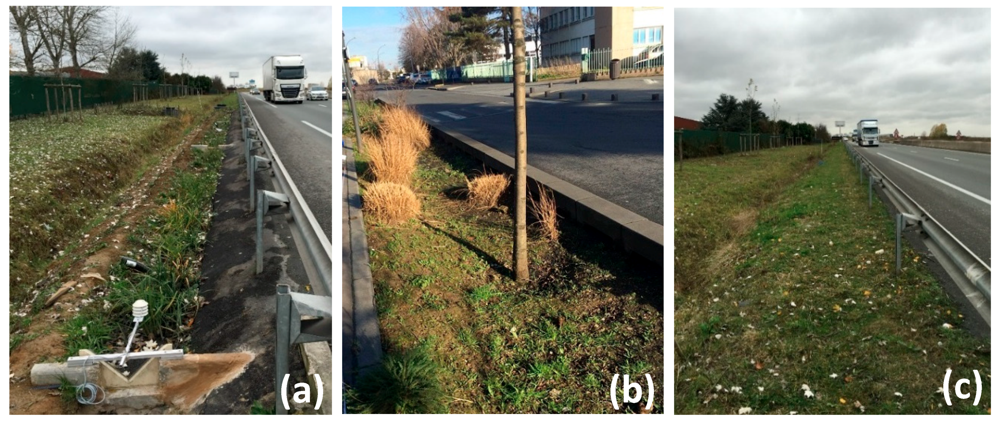
2.1. Study Sites

Three roadside SuDS in the Paris region (France) were chosen as the study sites. Sites A and B correspond to bioretention swales (Figure 1a,b) constructed in 2016 and 2006 respectively, whereas site C (Figure 1c) is a vegetated filter strip built in 2012. These types of SuDS are commonly used for road runoff management. Sites A and C are situated alongside a highway with high traffic; site B adjoins a T-junction in an industrial catchment. Site A is formed of a 48-cm-thick layer of filter media (40% v/v of natural soil mixed with 60% v/v of lime sand), drained at the bottom, and lined with an impervious geomembrane. Site C is composed of the same media, over a depth of approximately 20 cm, below which a drainage mat was placed. Site B was excavated to a depth of 60 to 70 cm and backfilled with a 40 cm × 40 cm gravel drainage trench around the tree pits, covered with topsoil taken from another site. Vegetation differs from one site to another: site A was planted with sedges; site B with grass, trees, and clumps; in site C, dense grass covers the whole filter strip. The dimensions of the devices are respectively 32, 20, and 50 m in length, and 0.7, 2, and 1.7 m in width.

The particle size distribution (PSD) was determined from a composite surface sample for each site (0–10 cm) with the sedimentation-Pipette method (NFX31-107). The coarse and fine sand fractions were separated via sieving at 0.2 mm and 50 µm, and the finest particles (clay and silt) were determined with a Robinson pipette. PSD results and associated textural classes are given in

Table 1. Particle size distribution and soil texture class of each site (results are given in % w/w).

	Site A (Surface)	Site A (20 cm)	Site B	Site C
Clay (<2 μm)	9.7	10.5	14.8	11.1
Fine silt (2–20 μm)	9.0	8.8	18.2	9.6
Coarse silt (20–50 μm)	9.2	11.1	21.9	18.6
Fine sand (50–200 μm)	15.4	18.2	17.6	13.5
Coarse sand (200–2000 μm)	56.7	51.4	27.5	47.2
Soil texture class (USDA)	Sandy Loam	Sandy Loam	Loam	Sandy Loam

. For site A, the particle size distribution was also established for a composite soil sample collected at a depth of 20-cm.

2.2. Soil Hydraulic Properties

Water flow in the vadose zone is highly influenced by soil hydraulic properties such as water retention curve $\mathsf{\theta }\left(\mathrm{h}\right)$ and hydraulic conductivity function $\mathrm{K}\left(\mathrm{h}\right)$, which can be described by various models. Among these, the van Genuchten model (Equations (1) and (2)), as well as the Brooks and Corey model (Equation (3)), are commonly used [21,22,23].

$$\mathsf{\theta }\left(\mathrm{h}\right)={\mathsf{\theta }}_{\mathrm{r}}+\frac{\left({\mathsf{\theta }}_{\mathrm{s}}-{\mathsf{\theta }}_{\mathrm{r}}\right)}{{\left[1+{\left|\frac{\mathrm{h}}{{\mathrm{h}}_{\mathrm{g}}}\right|}^{\mathrm{n}}\right]}^{\mathrm{m}}}$$

(1)

$$\mathrm{K}\left(\mathrm{h}\right)={\mathrm{K}}_{\mathrm{s}}{\left(\frac{\mathsf{\theta }\left(\mathrm{h}\right)-{\mathsf{\theta }}_{\mathrm{r}}}{{\mathsf{\theta }}_{\mathrm{s}}-{\mathsf{\theta }}_{\mathrm{r}}}\right)}^{1/2}{\left[1-{\left(1-{\left(\frac{\mathsf{\theta }\left(\mathrm{h}\right)-{\mathsf{\theta }}_{\mathrm{r}}}{{\mathsf{\theta }}_{\mathrm{s}}-{\mathsf{\theta }}_{\mathrm{r}}}\right)}^{1/\mathrm{m}}\right)}^{\mathrm{m}}\right]}^2$$

(2)

$$\mathrm{K}\left(\mathrm{h}\right)={\mathrm{K}}_{\mathrm{s}}{\left(\frac{\mathsf{\theta }\left(\mathrm{h}\right)-{\mathsf{\theta }}_{\mathrm{r}}}{{\mathsf{\theta }}_{\mathrm{s}}-{\mathsf{\theta }}_{\mathrm{r}}}\right)}^{\mathsf{\mu }}$$

(3)

where h (cm) is the pore water suction, θ(h) is the volumetric water content at the suction h, θ_r, and θ_s [cm³·cm⁻³] are respectively the residual and saturated volumetric water contents; K(h) is the hydraulic conductivity at the suction h, and K_s [m·s⁻¹] is the saturated hydraulic conductivity; $\mathrm{n}$, $\mathrm{m}$ and $\mathsf{\mu }$ are shape parameters; $\mathrm{m}$ can be calculated either as $\mathrm{m}=1-1/\mathrm{n}$ (Mualem’s condition [22]), or $\mathrm{m}=1-2/\mathrm{n}$ (Burdine’s condition [24]), and $\mathsf{\mu }=3+2/\left(\mathrm{n}-2\right)$ [24]; h_g [cm] is a scale parameter which corresponds approximately to the air entry bubbling pressure [25].

Among the indirect estimation methods of these parameters (θ_r, θ_s, K_s, h_g, $\mathrm{n}$), several pedotransfer functions may be found in the literature [26], such as the “Rosetta” software, based on the hierarchical relationships proposed by Schaap et al. [27]. Rosetta offers different options for the estimation of hydraulic soil properties, based on different levels of input data with increasing precision (1 = soil textural class only, 2 = soil texture, 3 = 2 + bulk density, 4 = 3 + one or two point(s) of the water retention curve corresponding to the field capacity and the wilting point) to predict the parameters of the van Genuchten-Mualem equations (Equations (1) and (2)). However, given the fact that soil hydraulic properties are affected by site-specific conditions like soil structure, macropores, and preferential flow paths [28], the applicability of pedotransfer functions which are based on a finite sample set may be limited. This is why field measurements are often recommended for more reliable and representative values.

2.3. Infiltration Tests

2.3.1. Type and Number of Infiltration Measurements

Site A underwent a complete characterization, focusing on both the horizontal and vertical variability of soil hydraulic properties, whereas the other two sites were investigated at the surface. For that purpose, two infiltration methods were used. The first is the Beerkan method [29] which consists of an in situ single ring infiltration test at the soil surface; the post-processing, usually referred to as the “BEST” algorithm, allows the soil hydraulic properties to be estimated (Equation (1) with Burdine’s condition and Equation (3)). The Beerkan method allows for measurements at the soil surface, without disturbing the soil. However, it is difficult to implement this method at a depth of 20 cm without excavating large volumes of soil and disrupting the bioretention system. A method that was less intrusive but with similar soil measurement volume had to be found. Thus, the determination of K_s in the sub-surface was performed with the mean of the Guelph permeameter [30].

Horizontal variability was assessed through a series of Beerkan infiltration experiments carried out at the surface of the three study sites, at equidistant locations, along a transect parallel to the road. The number of measurements at the surface of sites A, B, and C were 9, 10, and 9, respectively, which correspond to one measurement per 3.5, 2, and 6 m. For such infiltration systems, Ahmad et al. [13] and Cannavo et al. [31] have conducted one measurement per 14 m and 17.5 m, respectively, to balance effort (time and manpower) and accuracy. However, a higher density of infiltration measurements was retained in this study so as to evaluate spatial variability at a smaller scale. On site A, vertical variability was also evaluated, with 6 measurements carried out at a depth of 20 cm in the filter media, at 6 out of the 9 surface measurement locations.

2.3.2. Beerkan Infiltration Test and BEST Algorithm

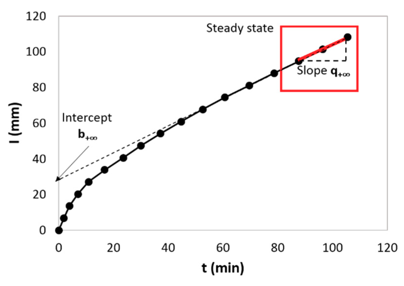
“Beerkan” In-Situ Infiltration Test

This method was adopted because it is simple, cost-effective, and easy, requiring a small volume of water and a short time; also, it does not disturb the soil surface. A cylinder was inserted to a depth of 1 cm into the soil. A given volume of water was applied repeatedly (100 or 50 mL in our case, depending on the site soil permeability), and the infiltration time of this volume was measured, until an apparent steady-state infiltration regime was reached, i.e., when three consecutive infiltration times were approximately identical. This step provided the cumulative infiltration curve of the soil. Given that the infiltration model in BEST algorithm [32] assumes a semi-infinite medium, the infiltration bulb should not reach lower boundary conditions before a steady state infiltration regime is reached. The dimension of the infiltration bulb depends on cylinder diameter [33], which should, therefore, be selected according to the depth of the filter media. In our case, two cylinders having a diameter of 50- and 97-mm were used respectively for site C and for sites A and B. Additionally, two 100 cm³ undisturbed soil samples were collected at each measurement point with soil sample rings; the first served to determine the soil bulk density and the initial volumetric water content (θ₀), and the other (taken at the end of the experiment) to estimate the saturated volumetric water content (θ_s) through a gravimetric method [34].

“BEST” Algorithm

In order to estimate the parameters of the water retention curve and hydraulic conductivity function, the “BEST” algorithm [32] was used. This algorithm relies on the inverse analysis of particle size distribution and the cumulative infiltration curve obtained by the Beerkan method described above, and assumes that θ_r = 0. Hydraulic shape parameters (n, m, and μ) derive from the analysis of both soil porosity and particle size distribution [32], while the scale parameters h_g and K_s are estimated from the inverse analysis of cumulative infiltration using the two-term equations developed by Haverkamp et al. [35]. Three algorithms can be used, referred to as “BEST-Slope”, “BEST-Intercept”, and “BEST-Steady” [36,37] which are different in defining the mathematical constraint between the sorptivity—capacity of the soil to absorb water by capillarity [38]—and the saturated hydraulic conductivity. The “BEST-Steady” was retained for the present analysis because it was proven to be a robust algorithm which always provides a proper estimate of K_s when the steady state infiltration regime could be reached [39].

BEST-Steady relies on the analytical expression of the slope (q_+∞) and the intercept (b_+∞) of the steady-state model (Equation (4)) fitted to the I(t) data at steady state conditions.

$$\mathrm{I}{\left(\mathrm{t}\right)}_{\mathrm{Steady}-\mathrm{state}}=\left[{\mathrm{K}}_{\mathrm{s}}+{\mathrm{AS}}^2\right]\mathrm{t}+\mathrm{C}\frac{{\mathrm{S}}^2}{{\mathrm{K}}_{\mathrm{s}}}$$

(4)

where I(t) is the cumulative infiltration at time t, S is the sorptivity, and A and C are constants of the cumulative infiltration model. The constraints between K_s and S are then defined based on the slope (Equation (5)) and intercept (Equation (6)) as follow:

$${\mathrm{K}}_{\mathrm{s}}={\mathrm{q}}_{+\infty }-{\mathrm{AS}}^2$$

(5)

$${\mathrm{K}}_{\mathrm{s}}=\mathrm{C}\frac{{\mathrm{S}}^2}{{\mathrm{b}}_{+\infty }}$$

(6)

Combining the latter two equations, S can be calculated as (Equation (7)):

$$\mathrm{S}=\sqrt{\frac{{\mathrm{q}}_{+\infty }}{\mathrm{A}+\frac{\mathrm{C}}{{\mathrm{b}}_{+\infty }}}}$$

(7)

Then K_s can be derived using either Equation (5) or (6).

2.3.3. Guelph Permeameter

In order to assess the vertical variability of the saturated hydraulic conductivity K_s, measurements were conducted at a depth of 20 cm using a Guelph permeameter. This method consists of measuring the steady-state infiltration rate in a small hole having a diameter-height of 6–20 cm, where a constant depth of water H is maintained [40]. The calculation method to evaluate K_s is fully described by Reynolds and Elrick [30], and the basic equation is given below (Equation (8)). At each measurement point, two ponding-depths H₁ (5 cm) and H₂ (10 cm) were established subsequently, for which two steady state infiltration rates, Q₁ and Q₂ respectively, were measured. Then, the two K_s values calculated using the single-height approach [41] were averaged.

$${\mathrm{K}}_{\mathrm{s}}=\frac{\mathrm{C}\mathrm{Q}}{2{\mathsf{\pi }\mathrm{H}}^2+{\mathsf{\pi }\mathrm{a}}^2\mathrm{C}+\raisebox{1ex}{$2\mathsf{\pi }\mathrm{H}$}\!\left/ \!\raisebox{-1ex}{${\mathsf{\alpha }}^{\ast }$}\right.}$$

(8)

where Q is the steady-state infiltration rate, H is the ponding depth, a is the well radius, C is a dimensionless shape factor that depends on H/a ratio, and α* is the ratio of gravity to capillarity forces [42].

2.4. Data Analysis

At first, the spatial variability of the measured data was quantified in terms of standard deviation and coefficient of variation. The uncertainties of the measurements obtained by the BEST algorithm, to experimental errors, were also assessed. Subsequently, Rosetta predictions for each site were compared to the measured values.

Lastly, the measured data of each site were tested for their statistical distribution. In previous experimental assessments, a log-normal distribution was often found to satisfactorily fit the collected data of saturated hydraulic conductivity [43,44]. Accordingly, the normality of ln(K_s) was tested by the means of Lilliefors test [45]. The null hypothesis of this test is that the data comes from a normal distribution. Results indicate the acceptance of the null hypothesis at a 5% significance level for the three sites. Thus, the K_s values of the sites A, B and C were fitted to a log-normal distribution. Fitting parameters obtained by the maximum likelihood estimation method are given in Figure A1, Appendix B.

2.5. Effect of K_s Variability on Hydrological Performance Modelling

The final aim of this study was to evaluate the effects of the spatial variability of soil hydraulic properties on the SuDS hydrologic modeling. This modelling approach may be useful to anticipate SuDS performance in the pre-construction phase, but also to verify their conformity with the preliminary design in the post-construction phase. As for the latter, the inherent spatial variability of soil hydraulic properties should be taken into consideration.

In order to study how the mean of K_s varies as a function of the number of measurements, an analysis was performed on the three sites. For each number of measurements N from 1 to 20, 1000 subsamples of size N were randomly sampled from the fitted log-normal distribution. Subsequently, the arithmetic mean of each subsample was computed, and the quantiles Q_0.1 and Q_0.9 of the latter 1000 means were determined. These quantiles were then normalized by the mean $m$ of the population. It should be noted that the mean $m$ of the population is calculated via the adjusted distribution for each site.

Additionally, a physically-based, one-dimensional model of a bioretention cell was conducted (Richard’s equation with the van Genuchten-Mualem relationships) to appraise the effects of various averaging methods of K_s, which account (or not) for its horizontal and/or vertical variability on the hydrological processes (focusing both on dynamical and cumulative aspects of the water balance).

Thus, multiple modelling approaches were tested, considering a theoretical device with comparable characteristics to those of site A (48 cm of sandy loam filter media, drained at the bottom, catchment/infiltration area ratio equal to 18, and pavement runoff coefficient of 0.9); water ponding at the surface of the cell is allowed over 17 cm.

The methodology consists of comparing the model outputs when only the surface K_s variability is considered on the one hand, and when the vertical variability is included on the other. In the first case, the considered K_s values are: (1) the mean m of the surface measurements; (2) the Rosetta predicted value; and lastly (3) the calculated quantiles Q_0.1 and Q_0.9 for a chosen N number of measurements. The vertical variability is accounted for with two additional approaches; firstly, a two-layered structure with different K_s, i.e., equal to the arithmetic mean of the total number of measurements at each layer; and secondly, a homogenous domain whose K_s is calculated as the harmonic mean of each layer’s K_s (Equation (9)), as suggested by Freeze and Cherry [46].

$${\mathrm{K}}_{\mathrm{s}}=\frac{\mathrm{d}}{{{\displaystyle \sum }}_{\mathrm{i}=1}^{\mathrm{n}}\frac{{\mathrm{d}}_{\mathrm{i}}}{{\mathrm{K}}_{\mathrm{si}}}}$$

(9)

where d is the total vertical thickness of all horizons, ${\mathrm{d}}_{\mathrm{i}}$ the thickness of each individual layer, ${\mathrm{K}}_{\mathrm{si}}$ the saturated hydraulic conductivity of the media in the individual layer, and n the total number of layers.

Simulations were run with the HYDRUS-1D software [47]. A 30-day series of rainfall and meteorological data including temperature, humidity, wind speed, and sunshine hours, recorded in the Paris region were used to compute the upper boundary condition. A water ponding depth was fixed at the surface, the excess water being considered as surface runoff (overflow). The lower boundary condition was chosen as a constant water content equal to the saturated water content of the soil. The parameters of the van Genuchten-Mualem relationships (

Table A2. van Genuchten-Mualem input parameters for HYDRUS 1D.

Van Genuchten Parameters	θr (cm3·cm−3)	θs (cm3·cm−3)	1/hg (cm−1)	n
At the surface	0.0395	0.23	0.044	1.4128
At 20 cm depth	0.0354	0.275	0.0552	1.2775

, Appendix C) were predicted with Rosetta PTFs based on the measured texture and bulk density, except for the K_s value, which depended on the modelling option.

3. Results and Discussion

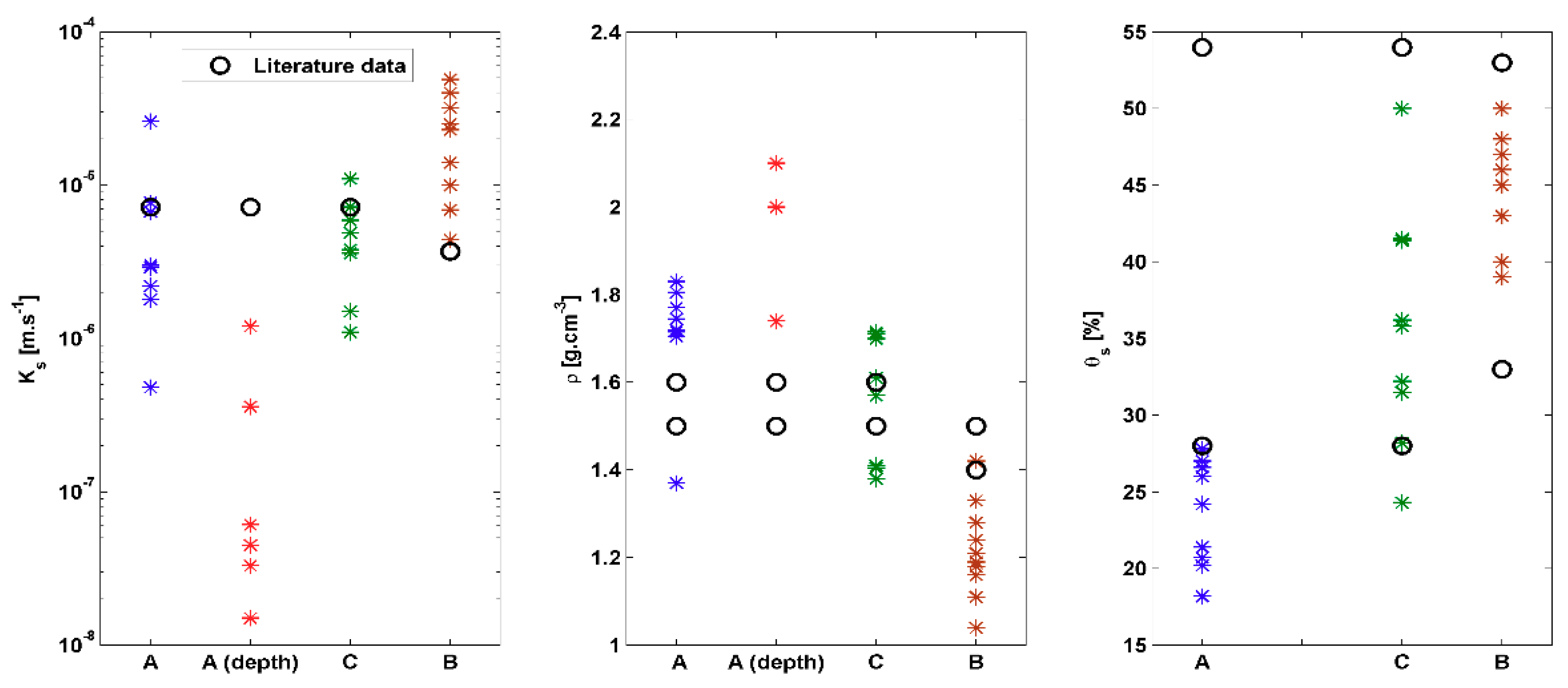
3.1. Horizontal and Vertical Variability of Soil Characteristics

The values of θ_s, 𝜌, and K_s measured at each point of the four sites are provided as Supplementary data (Appendix A); further developments are based on standard statistics (

Table 2. Statistics of the measured saturated water content θ_s, bulk density ρ, and saturated hydraulic conductivity K_s for the three sites.

		n	Min	Max	Median	SD	CV [%]	Arithmetic Mean
Site A Surface	θs [%]	9	18.2	27.8	24.2	3.5	15	23.6
	ρ [g·cm−3]	9	1.37	1.83	1.72	0.13	8	1.70
	Ks [m·s−1]	9	4.8 × 10−7	2.6 × 10−5	2.9 × 10−6	7.9 × 10−6	134	5.8 × 10−6
Site A (20 cm)	ρ [g·cm−3]	3	1.74	2.10	2.00	0.19	10	1.94
	Ks [m·s−1]	6	1.5 × 10−8	1.2 × 10−6	5.3 × 10−8	4.7 × 10−7	163	2.9 × 10−7
Site B	θs [%]	10	39	50	44	4.2	10	43.6
	ρ [g·cm−3]	10	1.04	1.42	1.20	0.10	9	1.22
	Ks [m·s−1]	10	4.4 × 10−6	4.9 × 10−5	1.9 × 10−5	1.5 × 10−5	70	2.1 × 10−5
Site C	θs [%]	9	24.3	50	35.8	7.8	22	35.7
	ρ [g·cm−3]	9	1.38	1.72	1.57	0.15	10	1.54
	Ks [m·s−1]	9	1.1 × 10−6	1.1 × 10−5	3.8 × 10−6	3 × 10−6	64	4.8 × 10−6

). Figure 2 illustrates the variability of these three parameters for the three sites. A comparison between the measurements and “typical” literature values (based on the texture class) of these soil properties is also presented. Literature data originate from more than 30 states in the USA [48]. The factors at the origin of the intra-site variability were discussed in this section, based on visual inspections as well as measurements.

Although sites A and C have similar textures (sandy loam), they display quite different saturated water content and bulk densities (Table 2). The values measured in site A are quite unusual in comparison with literature values, which may be the consequence of (i) a high compaction of the media during the construction of the swale; and (ii) the fact that the device is relatively recent—thus minimizing the long-term effects of vegetation growth and biological activity. Interestingly, both sites have very similar hydraulic conductivities at the surface: the arithmetic mean value of K_s in sites A and C is 5.8 × 10⁻⁶ and 4.8 × 10⁻⁶ m·s⁻¹, respectively, which is also consistent with literature data. Site B, which is formed of a loamy soil, has a lower density, and higher saturated water content and hydraulic conductivity than the two former sites. The mean K_s value is 2.1 × 10⁻⁵ m·s⁻¹, while “typical” values are one order of magnitude lower. This difference may be attributed to the types of vegetation present (trees and clumps) and their growth (10 years), so that the development of roots and biological activity may create macropores [49], which tend to increase the saturated hydraulic conductivity. The two latter examples suggest that soil texture may be an insufficient for a reliable estimation of soil hydraulic properties, since other factors such as construction technique, vegetation cover, and biological activity constitute additional sources of variability. To confirm these hypotheses, it would be of interest to undertake studies comparing sites with the same characteristics and their evolution over time.

Whatever the site, the soil saturated water content and bulk density did not display high variability: the associated coefficients of variation (CV) were lower than 22 and 10%, respectively. These results are in accordance with the previous findings of Nielsen et al. [50]. However, the variability associated to the K_s parameter (at the surface) was found to be much higher, with a coefficient of variation ranging from 64% in site C to 134% in site A. In the latter case, there was visual evidence of an uneven distribution of the vegetation, which explain this higher variability [51]. The present results should be put into perspective with the findings of Mulla et al. and Vauclin et al. [52,53] who reported a coefficient of variation ranging from 48 to 352% for K_s; additionally Warrick [54] pointed out low variability of the bulk density and saturated water content (<15%) and high variability of saturated hydraulic conductivity (>50%).

With regards to the variation of the K_s parameter at the surface, it should be noted that no spatial trend was visible with respect to the longitudinal location within the swales or the filter strip. Contrariwise, the measurements at a depth of 20 cm were more than one order of magnitude lower than at the surface (Table 2), evidencing a vertical variability of K_s; this difference could be induced by the different infiltration test methods (Beerkan at the surface, Guelph at 20 cm). While Guelph was found to produce lower K_s measurements than other infiltration tests that explore a larger soil volume [55,56], no comparison was found in the literature to the Beerkan test, which explores a similar soil volume. The lower infiltration rates at 20 cm are consistent with other field observations. Firstly, a difference of compaction between the two layers was noted, as shown by the vertical increase in bulk density (from 1.70 to 1.94 g·cm⁻³) with depth. As for this cause, Pitt et al. [57] have demonstrated that the saturated hydraulic conductivity of soil is highly affected by the degree of compaction. In the latter study, a sandy loam soil with a bulk density of 2 g·cm⁻³ was found to have a saturated hydraulic conductivity of 8 × 10⁻⁸ m·s⁻¹. The construction techniques may induce this level of compaction since for site A, the filter media was placed on a smooth geomembrane. Actually, a smooth underlying layer causes a significant decrease in saturated water content, as tested by Brown and Hunt [58]. In addition, the filter media was implemented in wet conditions, which may also have a strong impact on the degree of compaction, and subsequently, on the steady-state infiltration rate of the soil.

In order to further investigate the factors which may cause this significant decrease in K_s with increasing depth, 3 soil samples were composited from 6 subsamples collected respectively at the surface, 20 cm, and 30 cm depth in the bioretention swale; these samples were then analyzed for both their particle size distribution and their total calcium carbonate content. The results revealed no significant difference in particle size distribution with depth, negating the hypothesis of downward migration of fine particles. Conversely, the CaCO₃ increased with increasing depth, from 214 g/kg at the surface to 252 and 265 g/kg at 20 and 30 cm, respectively. As the sand used in the filter media mixture is basically calcareous, the decrease in saturated hydraulic conductivity and the increase in the bulk density might be due to CaCO₃ precipitation that “plugs” soil pores [59].

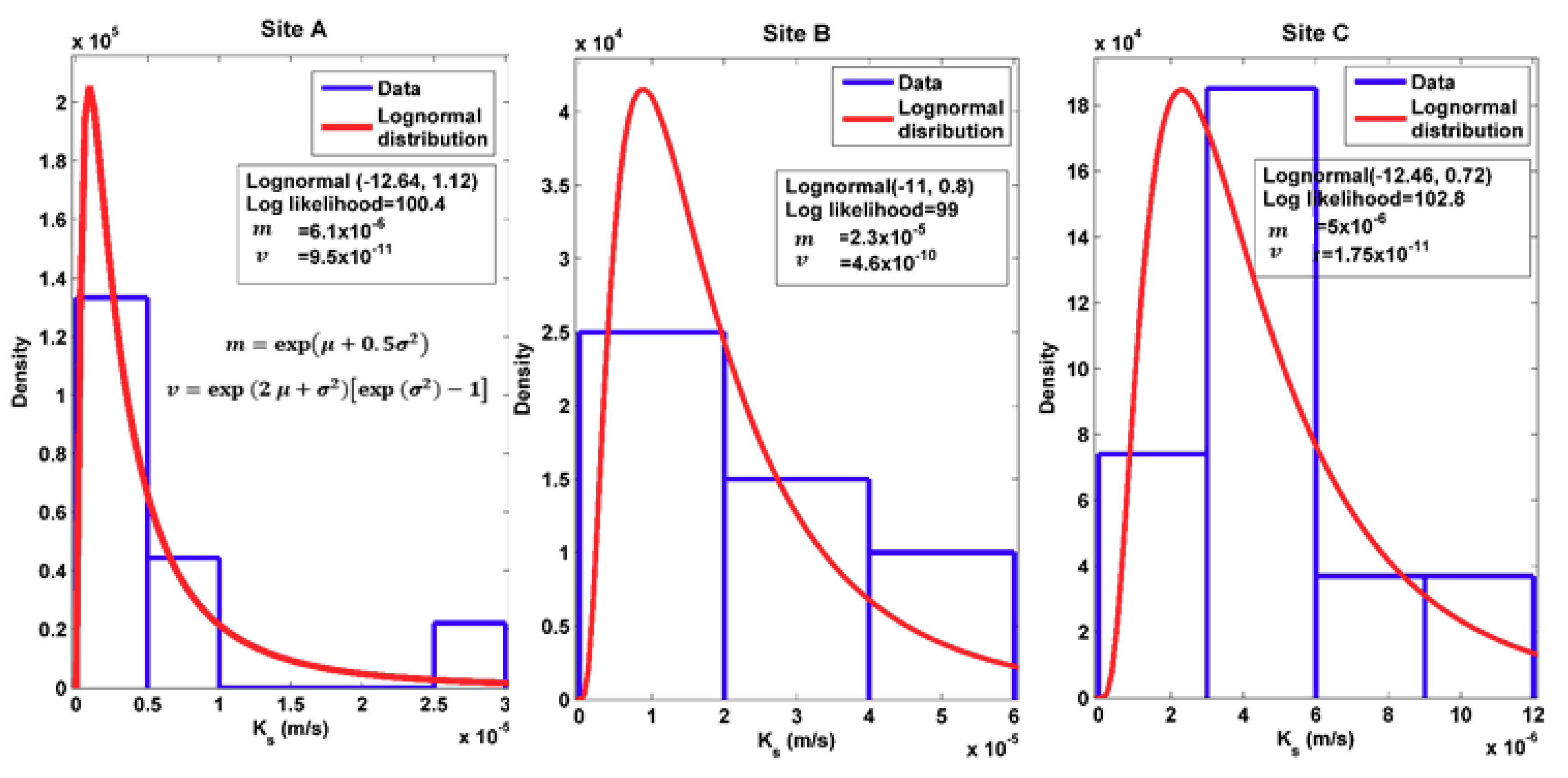
3.2. Measurement Uncertainties

The spatial variability of the saturated hydraulic conductivity at the surface should be compared with potential errors in the experimental measurements, which might also induce biases in the values determined by the “BEST” algorithm. Sensitivity analyses of the algorithm to experimental conditions have been the subject of multiple previous studies. One of these is Di Prima et al. [39], who stated that the BEST method leads to a good estimation when the prescribed conditions are respected (e.g., the attainment of the steady state). This section is dedicated to assessing the sensitivity of this algorithm to its input data (i.e., the initial water content θ₀, bulk density ρ, and particle size distribution) when the experimental conditions are respected, but considering the possible occurrence of experimental errors. For example, a wrong estimation of θ₀ and ρ may be the consequence of a non-complete cylinder taken at the beginning of the test. Additionally, these two parameters might show “local” variability, i.e., at a very small scale, inducing differences between the point where infiltration was conducted and the adjacent point where the cylinder was taken. This spatial variability was quantified during this study by collecting 5 samples at a small scale. It was found to be equal to ±0.05 cm³∙cm⁻³ and ±0.1 g∙cm⁻³ for θ₀ and ρ, respectively. Assuming that the soil texture does not vary at this scale and that the cumulated infiltration curve (Figure 3) was assessed precisely, the two remaining sources of experimental errors are θ₀ and ρ, the effects of which will be discussed in the following developments.

Figure 4 presents the sensitivity of the estimated hydraulic conductivity to θ₀ and ρ for four tests (carried out in sites A, B, and C) with different initial conditions. Tests B3 and C1 were conducted in a soil with relatively low bulk density (1.28 and 1.38 g·cm⁻³, respectively), at different initial water contents (19% and 28.5% respectively), while for the other two tests, A6 and C6, the bulk density was higher (1.72 and 1.70 g·cm⁻³, respectively) and the initial water content was equal to 8.1% and 27.3% respectively.

It should be kept in mind that Figure 4 does not represent the dependency of K_s upon the soil parameters, but the dependency of the estimation method (i.e., the “BEST-steady” algorithm) on its measured input data. Hence, for a given infiltration curve, the predicted K_s decreases with increasing θ₀ and ρ. Results show that for the four measurement points, the error in the predicted hydraulic conductivity due to a ±0.05 cm³∙cm⁻³ variation in θ₀ is larger than the error induced by ±0.1 g∙cm⁻³ variation in ρ. For example, for point B3, these errors represent 13% and 9.5% of the K_s measurement value, respectively. For tests A6 and B3, an error of ±0.05 cm³∙cm⁻³ in the initial water content causes an error of 12% and 13% of the K_s measurement values, respectively. With regards to the points C1 and C6, which display the highest bulk densities and the lowest hydraulic conductivities among these four examples, the potential bias induced by a ±0.05 cm³∙cm⁻³ error in the initial water content corresponds respectively to 23% and 32% of the calculated K_s value.

Therefore, the “BEST-Steady” algorithm appears to be a precise and robust tool to predict the soil’s saturated hydraulic conductivity; yet, it is more sensitive to experimental errors if the soil is initially near saturation, especially for high bulk density soils. In all cases, the potential error related to a wrong but probable measurement of θ₀ or ρ is lower than the coefficient of variation of K_s within each site.

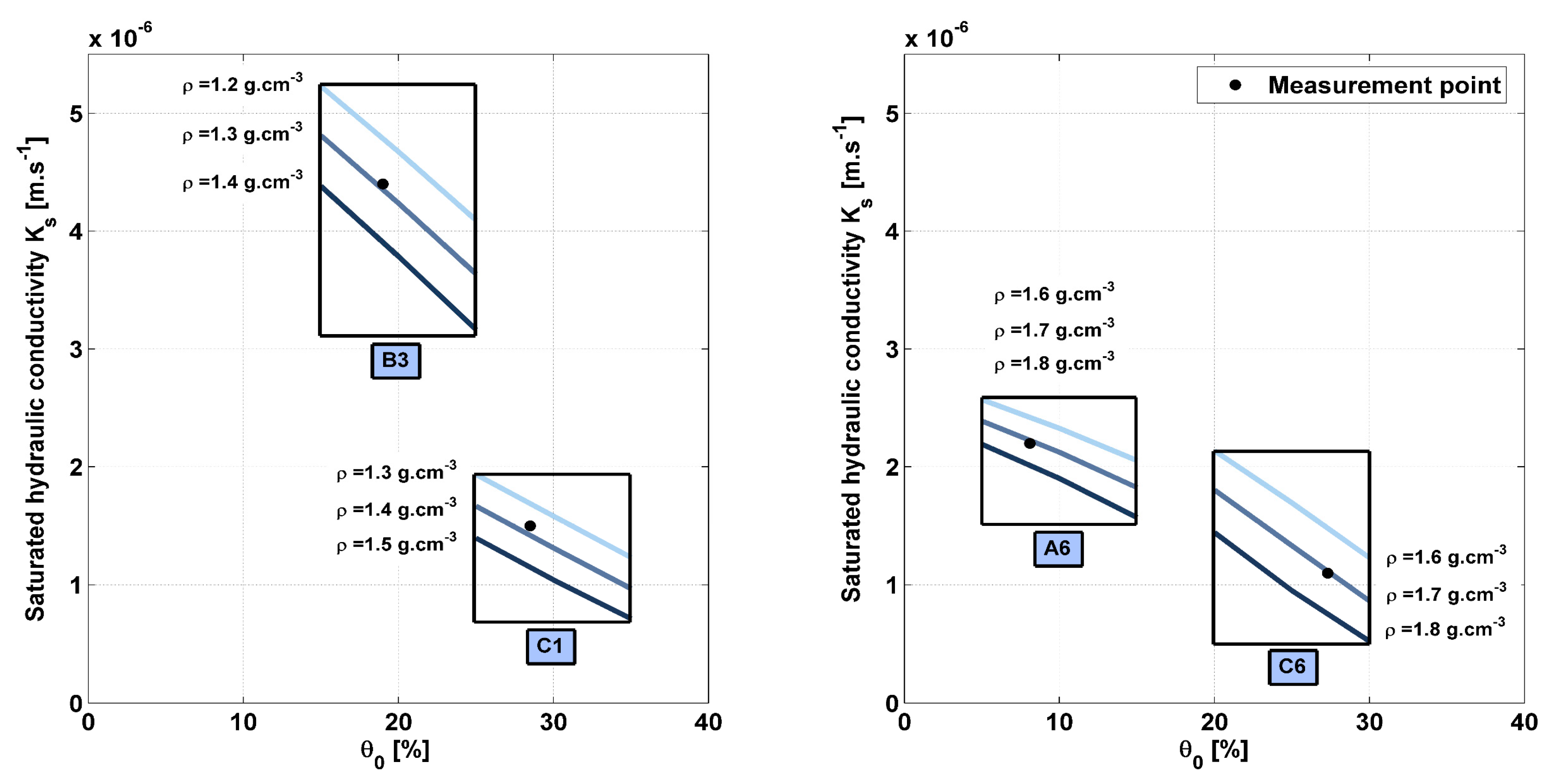
3.3. The Accuracy of the Pedotransfer Functions

In order to emphasize potential differences between the estimation methods of the curves $\mathrm{K}\left(\mathrm{h}\right)$ and $\mathsf{\theta }\left(\mathrm{h}\right)$, three characteristic points of these relationships were evaluated—describing the state of soil under saturated conditions, the field capacity (h = 2.5 pF), and wilting point (h = 4 pF) [60]—after assessing the soil hydraulic parameters of the four sites via Rosetta and the “BEST” algorithm, respectively. Three pedotransfer functions were tested, which used different input data: (i) textural class; (ii) particle size analysis; and (iii) particle size analysis and average bulk density measured in the field. The results are shown in

Table 3. Comparison between Rosetta estimations and experimental measurements of the curves K (h) and θ (h) (mean (standard deviation) of all the measurements carried out in each site).

		Permeability Curve K(h) (m·s−1)			Retention Curve θ(h) (%)
		Ks	K (2.5 pF)	K (4 pF)	θs	θ (2.5 pF) θ/θs (%)	θ (4 pF) θ/θs (%)
Site A	Rosetta (Textural class)	4.4 × 10−6	5.1 × 10−10	1.1 × 10−14	38.7	14.7 38	3.2 8
	Rosetta (%Sand, Silt, Clay)	5.8 × 10−6	2.6 × 10−10	5.7 × 10−15	38.4	12.7 33	2.7 7
	Rosetta (%Sand, Silt, Clay + ρ)	2.9 × 10−6	8.0 × 10−11	2.5 × 10−15	33.0	11.2 34	2.8 8
	Mean BEST values	5.9 × 10−6 (7.9 × 10−6)	3.4 × 10−10 (5.8 × 10−10)	3.0 × 10−14 (5.1 × 10−14)	23.5 (3.5)	9.6 (1.9) 40	4.2 (0.9) 18
Site B	Rosetta (Textural class)	1.4 × 10−6	2.1 × 10−9	4.4 × 10−14	39.9	21.0 53	4.3 10
	Rosetta (%Sand, Silt, Clay)	1.7 × 10−6	3.0 × 10−9	5.3 × 10−14	39.6	20.7 52	4.0 10
	Rosetta (%Sand, Silt, Clay + ρ)	4.8 × 10−6	1.5 × 10−8	1.7 × 10−13	42.5	22.7 53	3.6 8
	Mean BEST values	2.1 × 10−5 (1.5 × 10−5)	4.0 × 10−9 (7.1 × 10−9)	4.6 × 10−13 (8.0 × 10−13)	43.6 (4.2)	20.4 (2.8) 47	9.9 (1.4) 23
Site C	Rosetta (Textural class)	4.4 × 10−6	5.1 × 10−10	1.1 × 10−14	38.7	14.7 38	3.2 8
	Rosetta (%Sand, Silt, Clay)	3.9 × 10−6	5.7 × 10−10	1.9 × 10−14	38.7	16.543	4.2 10
	Rosetta (%Sand, Silt, Clay + ρ)	3.3 × 10−6	3.7 × 10−10	1.1 × 10−14	36.6	14.8 40	3.6 10
	Mean BEST values	4.8 × 10−6 (3.0 × 10−6)	5.9 × 10−10 (9.4 × 10−10)	5.5 × 10−14 (8.8 × 10−14)	35.7 (7.8)	16.0 (4.4) 45	7.3 (2.0) 20

.

Regarding the saturated hydraulic conductivity in sites A and C, the maximum difference between Rosetta estimation and “BEST” prediction is 3.0 × 10⁻⁶ and 1.5 × 10⁻⁶ m·s⁻¹, respectively, which falls within the measured spatial variability of this parameter in these two devices, but is higher than the experimental bias evaluated in Section 3.2. In site B, where pedotransfer functions underestimate K_s, the maximum difference is 1.9 × 10⁻⁵ m·s⁻¹, while the standard deviation of the measurements is 1.5 × 10⁻⁵ m·s⁻¹. In this site, the development of vegetation roots over time may have caused modifications in the soil structure that were not taken into consideration in the PTFs functions [61]. Yet, it appears that the accuracy of Rosetta predictions does not necessarily increase with increasing precision of the input data (e.g., in site A, the mean K_s is better predicted without adding the bulk density, and in site C, it is better predicted with the textural class only). Following a similar approach (based on laboratory measurements of K_s on undisturbed soil samples from an agricultural field), [62] came to the same conclusion—as long as the 4th hierarchical level of input data (i.e., including textural class, soil texture, bulk density and the water content at field capacity) was not reached.

The preceding remarks also apply to the hydraulic conductivity at field capacity and wilting point K (2.5 pF) and K (4 pF): Rosetta predictions fall within the spatial variability for sites A, B, and C.

As for the retention curve, pedotransfer functions appear to be quite accurate in predicting θ_s and θ (2.5 pF) for sites B and C; however, the measured values in site A are significantly lower than the Rosetta prediction, whatever the input data. This observation is a probable consequence of the unusually high bulk density in this infiltration system (1.7–1.9 g·cm⁻³), which significantly decreased the soil’s porosity. In order to further assess the predictive capacity of the Rosetta model, the comparison was realized based on effective saturation θ/θ_s (%). The latter measure expresses the shape parameter n and scale parameter h_g of the van Genuchten model. At 2.5 pF, the maximum differences in effective saturation between Rosetta and BEST for the three sites are equal to 5% to 7%. However, at 4 pF, the two estimation methods lead to different values and higher differences in effective saturation (11% to 15%), which may be related to intrinsic differences between the van Genuchten-Mualem and the van Genuchten with Burdine’s condition models, resulting in non-overlaying curves at high-pressure heads.

Hence, pedotransfer functions globally appear to be relevant tools for estimating K_s when the natural variability of this parameter is not important and the structure of the soil is marginally affected by either long-term factors such as vegetation growth or short-term conditions as a construction technique.

3.4. Effect of Horizontal and Vertical Variability of Soil Hydraulic Properties on the Hydrological Performance

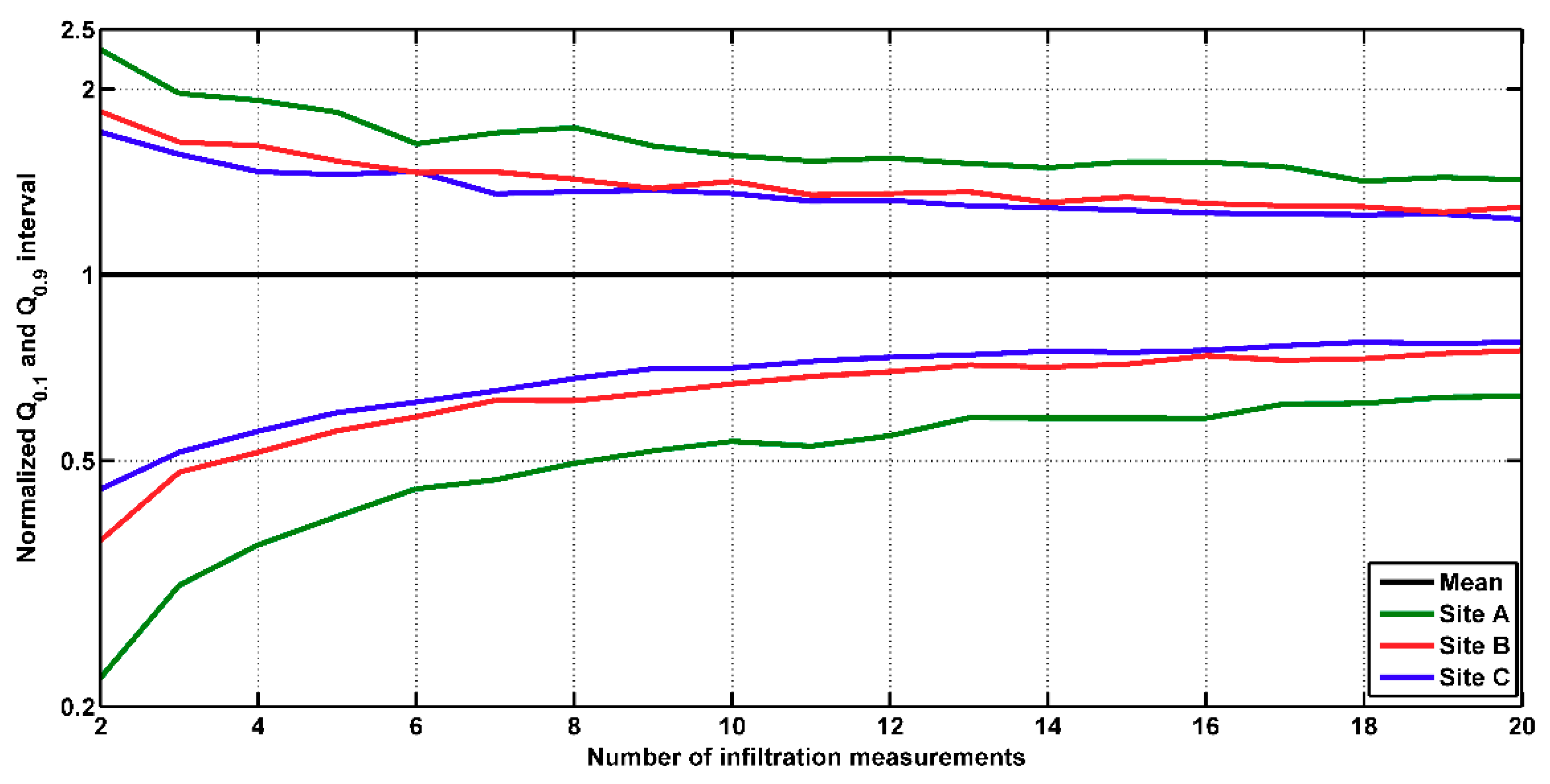
3.4.1. Number of Infiltration Measurements Needed for a Representative Value of K_s

The quantiles Q_0.1 and Q_0.9 normalized by the mean $m$ of the population are plotted as a function of the sample size for the three sites A, B, and C in Figure 5. These quantiles constitute an empirical 80% confidence interval which represents the uncertainty in the estimation of K_s mean value from N measurements.

This uncertainty on the evaluation of K_s arithmetic mean decreases with an increasing number of measurements. For example, considering a small number of measurements n = 2, it is equal to a factor of 2–3. Yet, with a larger number of measurement n = 8, this uncertainty decreases to a factor <2, for all three sites. Additionally, the quantiles intervals show an asymptotic behavior, starting from a certain number of measurements. Thus, an increase in infiltration measurements beyond this certain number does not necessarily yield a better evaluation of K_s.

Actually, site A presents a high dispersion of the measured values; as a reminder, the coefficient of variation of K_s was 134%, while this variation was <70% for sites B and C. Hence the uncertainty on K_s mean associated with N measurements for the latter two sites is lower than for site A. This variation from one site to another is due to the dispersion parameters of the log-normal distribution that derive directly from spatial variability of K_s within each site.

Therefore, the number of infiltration measurements depends on two factors: the required level of uncertainty on K_s evaluation and the studied site. For an uncertainty of a factor of two or less, which is operationally acceptable, this number is equal to 4 (resp. 8) measurements for sites B and C (resp. site A). This brings into question the consequence of this level of uncertainty on the hydrological modelling of SuDS.

3.4.2. Effect of the Horizontal and Vertical Variability of Soil Hydraulic Properties on the Hydrological Modelling

Modelling results including drained fluxes and cumulated drained/runoff volumes are shown in Figure 6. The considered K_s values in the different scenarios are equal to (1) the mean m of the surface measurements (6.1 × 10⁻⁶ m∙s⁻¹); (2) the Rosetta predicted value based on the particle size distribution (5.8 × 10⁻⁶ m∙s⁻¹); and lastly (3) the quantiles calculated in Section 3.4.1 (Q_0.1 (3 × 10⁻⁶ m∙s⁻¹) and Q_0.9 (1 × 10⁻⁵ m∙s⁻¹) for n = 8, corresponding to an uncertainty of a factor of two for site A). With regards to the vertical variability, the average K_s value at 20 cm and the harmonic mean are equal to 2.9 × 10⁻⁷ m∙s⁻¹ and 4.8 × 10⁻⁷ m∙s⁻¹, respectively.

Regarding simulations considering only the surface measurements, results show a variation in dynamic fluxes when K_s values vary. The peaks and troughs corresponding to the mean of the population and Rosetta prediction (referred to as Mean 1 L and Rosetta 1 L, respectively) are very similar: their peaks are around 400 L∙h⁻¹. However, these peaks decrease (resp. increase) by a factor of 2 when K_s value is equal to the quantile Q_0.1 (resp. Q_0.9). Although an increase in K_s value by a factor of 1.6 results in a notable increase in peak fluxes, it does not necessarily induce a remarkable increase in the cumulated drained volume, which amounts to ∼4 × 10⁴ L at the end of the simulation period for the mean, Rosetta, and Q_0.9. In contrast, a decrease in K_s value as for Q_0.1 has an impact on the cumulated drained volume, since it allows more water accumulation on the surface, leading to the generation of runoff (overflow) when the depth of water exceeds the available ponding depth. Therefore, a threshold is observed in the impact of K_s on the outputs, corresponding to the moment where the surface water exceeds the available ponding-depth.

Regarding the vertical variability, the outputs of a two-layered system with an attributed K_s for each layer is referred to as Mean 2 L, while the homogeneous layer with a harmonic mean K_s is referred to as Harmonic mean 1 L. At first, the results revealed no significant differences in dynamics and fluxes between the two-layered model and the homogeneous layer model. However, when comparing, the latter two approaches that account for vertical variability to the previous approaches that consider only the surface horizontal variability, large gaps in their outputs are identified. For instance, the inclusion of vertical variability in the model either by a two-layered or one layer domain sharply reduces the peak drained flux by a factor of 12. Additionally, the infiltration dynamics are completely smoothed and the drainage time is no longer comparable. The latter increased from several hours to several days (7 to 10 days) for the Mean 1L and the Mean 2 L/Harmonic mean 1 L, respectively. The vertical variability also has implications on the water balance. To illustrate this statement, the drained volumes constitute >80% of the water volumes and the runoff <20% if only the surface measurements are considered, whereas their relative importance is inverted when the vertical variability is considered (30% and 70%, respectively).

Therefore, results significantly emphasize the impact of vertical variability on the model outputs. Neglecting this variability when it exists might introduce discrepancies in the overall simulations results. The effect of a layer having very low K_s is better accounted for by a harmonic mean of each layer’s K_s than by a simple arithmetic mean. Thus, a homogenous domain whose K_s is equal to a harmonic mean could replace a two-layered system. Consequently, factors causing this variability, such as construction techniques inducing high compaction level in addition to the type of sand used in the media (as discussed in Section 3.1), may cause an important variation in the SuDS’ hydrologic performance. This prevents the facility from mimicking the pre-development conditions in order to mitigate peaks inflow without producing overflow.

4. Conclusions

Uncertainty in soil hydraulic properties related to evaluation/measurement method, as well as intrinsic horizontal and vertical variability, were investigated in this paper for three roadside sustainable drainage systems (SuDS). Analysis of factors affecting this variability, as well as its effects on the simulated water dynamics and volumes, was achieved.

The horizontal variability of the saturated hydraulic conductivity was found to be high, with a coefficient of variation ranging from 60% to 160% within each device, without any visible spatial trend. Additionally, a notable vertical variability was found in one of the studied sites (the bioretention swale). Construction techniques (compaction), uneven development of vegetation and biological activity, operating time, as well as calcium carbonate precipitation, could play an important role on soil hydraulic properties values and their spatial variability.

Spatial variability of the soil hydraulic properties was found to be dominant relative to the uncertainties in PTFs predictions and those induced by the experimental errors. The PTFs predict the water retention and hydraulic conductivity curves with reasonable accuracy for two sites out of three.

The number of infiltration measurements that might be conducted in order to accurately evaluate the arithmetic mean of K_s with an uncertainty of a factor of two or less and at 80% confidence level was found to be four/eight, depending on the studied site.

The effect of horizontal and vertical variability of the K_s value on the predicted hydrologic performance of a bioretention cell was assessed using the HYDRUS-1D software. The results clearly highlight the significant impact of K_s on the simulated water dynamics, including drained flux and volume. In addition, the vertical variability was found to be the most impacting relative to the horizontal variability of K_s and its assessment method. This vertical variability could modify the long-term hydrologic performance of SuDS and the flow apportionment by decreasing infiltration into the soil and increasing the overland flow. Consequently, to effectively represent the spatial variability when modeling an infiltration SuDS, soil measurements should be conducted at the surface, and vertically as well. A harmonic mean value of each layer’s K_s applied to a homogenous domain could be an alternative to a two-layered domain with two different K_s.

In this study, the temporal variability of soil hydraulic properties was not investigated. An in-depth investigation of this variability and its dependency on the climate, maintenance techniques, and other temporal factors such as biological activity and highway sediment deposition, would also be needed. Such an investigation would be helpful in the development of hydrological models by promoting the implementation of time-variable soil hydraulic properties.

References

1. Coombes, P.J.; Kuczera, G.; Kalma, J.D.; Argue, J.R. An evaluation of the benefits of source control measures at the regional scale. Urban Water 2002, 4, 307–320. [Google Scholar] [CrossRef]
2. Liu, A.; Goonetilleke, A.; Egodawatta, P. Taxonomy for rainfall events based on pollutant wash-off potential in urban areas. Ecol. Eng. 2012, 47, 110–114. [Google Scholar] [CrossRef] [Green Version]
3. Davis, A.P. Green Engineering Promote Low-Impact Development. Environ. Sci. Technol. 2005, 39, 338A–344A. [Google Scholar] [CrossRef] [PubMed]
4. Davis, A.P. Field Performance of Bioretention: Hydrology Impacts. J. Hydrol. Eng. 2008, 13, 90–95. [Google Scholar] [CrossRef] [Green Version]
5. Bäckström, M.; Viklander, M.; Malmqvist, P.-A. Transport of stormwater pollutants through a roadside grassed swale. Urban Water J. 2006, 3, 55–67. [Google Scholar] [CrossRef]
6. Barrett, M.E.; Walsh, P.M.; Malina, J.F., Jr.; Charbeneau, R.J. Performance of Vegetative Controls for Treating Highway Runoff. J. Environ. Eng. 1998, 124, 1121–1128. [Google Scholar] [CrossRef]
7. Deletic, A.; Fletcher, T.D. Performance of grass filters used for stormwater treatment—A field and modelling study. J. Hydrol. 2006, 317, 261–275. [Google Scholar] [CrossRef]
8. Rezaei, M.; Seuntjens, P.; Joris, I.; Boënne, W.; Van Hoey, S.; Campling, P.; Cornelis, W.M. Sensitivity of water stress in a two-layered sandy grassland soil to variations in groundwater depth and soil hydraulic parameters. Hydrol. Earth Syst. Sci. Discuss. 2015, 12, 6881–6920. [Google Scholar] [CrossRef]
9. Clothier, B.E.; Smettem, K.R.J. Combining laboratory and field measurements to define the hydraulic properties of soil. Soil Sci. Soc. Am. J. 1990, 54, 299–304. [Google Scholar] [CrossRef]
10. Jhorar, R.K.; Van Dam, J.C.; Bastiaanssen, W.G.M.; Feddes, R.A. Calibration of effective soil hydraulic parameters of heterogeneous soil profiles. J. Hydrol. 2004, 285, 233–247. [Google Scholar] [CrossRef]
11. Angulo-Jaramillo, R.; Vandervaere, J.-P.; Roulier, S.; Thony, J.-L.; Gaudet, J.-P.; Vauclin, M. Field measurement of soil surface hydraulic properties by disc and ring infiltrometers: A review and recent developments. Soil Tillage Res. 2000, 55, 1–29. [Google Scholar] [CrossRef]
12. Reynolds, W.D.; Elrick, D.E.; Youngs, E.G.; Booltink, H.W.G.; Bouma, J.; Dane, J.H. Saturated and Field-Saturated Water Flow Parameters: Laboratory methods. In Methods of Soil Analysis; Soil Science Society of America: Madison, WI, USA, 2002; pp. 688–690. [Google Scholar]
13. Ahmed, F.; Gulliver, J.S.; Nieber, J.L. Field infiltration measurements in grassed roadside drainage ditches: Spatial and temporal variability. J. Hydrol. 2015, 530, 604–611. [Google Scholar] [CrossRef]
14. Weiss, P.T.; Gulliver, J.S. Effective saturated hydraulic conductivity of an infiltration-based stormwater control measure. J. Sustain. Water Built Environ. 2015, 1, 04015005. [Google Scholar] [CrossRef]
15. Jabro, J.D.; Iversen, W.M.; Stevens, W.B.; Evans, R.G.; Mikha, M.M.; Allen, B.L. Physical and hydraulic properties of a sandy loam soil under zero, shallow and deep tillage practices. Soil Tillage Res. 2016, 159, 67–72. [Google Scholar] [CrossRef]
16. Logsdon, S.D. CS616 Calibration: Field versus Laboratory. Soil Sci. Soc. Am. J. 2009, 73, 1. [Google Scholar] [CrossRef]
17. Marín-Castro, B.E.; Geissert, D.; Negrete-Yankelevich, S.; Gómez-Tagle Chávez, A. Spatial distribution of hydraulic conductivity in soils of secondary tropical montane cloud forests and shade coffee agroecosystems. Geoderma 2016, 283, 57–67. [Google Scholar] [CrossRef]
18. Sobieraj, J.A.; Elsenbeer, H.; Coelho, R.M.; Newton, B. Spatial variability of soil hydraulic conductivity along a tropical rainforest catena. Geoderma 2002, 108, 79–90. [Google Scholar] [CrossRef]
19. Mubarak, I.; Angulo-Jaramillo, R.; Mailhol, J.C.; Ruelle, P.; Khaledian, M.; Vauclin, M. Spatial analysis of soil surface hydraulic properties: Is infiltration method dependent? Agric. Water Manag. 2010, 97, 1517–1526. [Google Scholar] [CrossRef]
20. Rienzner, M.; Gandolfi, C. Investigation of spatial and temporal variability of saturated soil hydraulic conductivity at the field-scale. Soil Tillage Res. 2014, 135, 28–40. [Google Scholar] [CrossRef]
21. Brooks, R.; Corey, T. Hydraulic Properties of Porous Media; Hydrology Papers Colorado State University: Fort Collins, CO, USA, 1964. [Google Scholar]
22. Mualem, Y. A new model for predicting the hydraulic conductivity of unsaturated porous media. Water Resour. Res. 1976, 12, 513–522. [Google Scholar] [CrossRef]
23. van Genuchten, M.T. A Closed-form Equation for Predicting the Hydraulic Conductivity of Unsaturated Soils1. Soil Sci. Soc. Am. J. 1980, 44, 892. [Google Scholar] [CrossRef]
24. Burdine, N. Relative permeability calculations from pore size distribution data. J. Pet. Technol. 1953, 5, 71–78. [Google Scholar] [CrossRef]
25. Bouwer, H. Rapid field measurement of air entry value and hydraulic conductivity of soil as significant parameters in flow system analysis. Water Resour Res 1966, 2, 729–738. [Google Scholar] [CrossRef]
26. McBratney, A.B.; Minasny, B.; Cattle, S.R.; Vervoort, R.W. From pedotransfer functions to soil inference systems. Geoderma 2002, 109, 41–73. [Google Scholar] [CrossRef]
27. Schaap, M.G.; Leij, F.J.; Van Genuchten, M.T. ROSETTA: A computer program for estimating soil hydraulic parameters with hierarchical pedotransfer functions. J. Hydrol. 2001, 251, 163–176. [Google Scholar] [CrossRef]
28. Lin, H.S.; McInnes, K.J.; Wilding, L.P.; Hallmark, C.T. Effects of Soil Morphology on Hydraulic Properties. Soil Sci. Soc. Am. J. 1999, 63, 955. [Google Scholar] [CrossRef]
29. Lassabatère, L.; Angulo-Jaramillo, R.; Winiarski, T.; Yilmaz, D. Advances in Unsaturated Soils. In BEST Method: Characterization of Soil Unsaturated Hydraulic Properties; CRC Press Taylor and Francis Group: London, UK, 2013. [Google Scholar]
30. Reynolds, W.D.; Elrick, D.E. In situ measurement of field-saturated hydraulic conductivity, sorptivity, and the α-parameter using the Guelph permeameter. Soil Sci. 1985, 140, 292–302. [Google Scholar] [CrossRef]
31. Cannavo, P.; Coulon, A.; Charpentier, S.; Béchet, B.; Vidal-Beaudet, L. Water balance prediction in stormwater infiltration basins using 2-D modeling: An application to evaluate the clogging process. Int. J. Sediment Res. 2018. [Google Scholar] [CrossRef]
32. Lassabatère, L.; Angulo-Jaramillo, R.; Soria Ugalde, J.M.; Cuenca, R.; Braud, I.; Haverkamp, R. Beerkan Estimation of Soil Transfer Parameters through Infiltration Experiments—BEST. Soil Sci. Soc. Am. J. 2006, 70, 521. [Google Scholar] [CrossRef]
33. Reynolds, W.D.; Elrick, D.E. Ponded infiltration from a single ring: I. Analysis of steady flow. Soil Sci. Soc. Am. J. 1990. [Google Scholar] [CrossRef]
34. Topp, G.C.; Ferré, P.A. 3.1 Water content. In Methods of Soil Analysis; Soil Science Society of America: Madison, WI, USA, 2002; pp. 417–545. [Google Scholar]
35. Haverkamp, R.; Ross, P.J.; Smettem, K.R.J.; Parlange, J.Y. Three-dimensional analysis of infiltration from the disc infiltrometer: 2. Physically based infiltration equation. Water Resour. Res. 1994, 30, 2931–2935. [Google Scholar] [CrossRef] [Green Version]
36. Bagarello, V.; Di Prima, S.; Iovino, M. Comparing Alternative Algorithms to Analyze the Beerkan Infiltration Experiment. Soil Sci. Soc. Am. J. 2014, 78, 724. [Google Scholar] [CrossRef]
37. Yilmaz, D.; Lassabatere, L.; Angulo-Jaramillo, R.; Deneele, D.; Legret, M. Hydrodynamic Characterization of Basic Oxygen Furnace Slag through an Adapted BEST Method. Vadose Zone J. 2010, 9, 107. [Google Scholar] [CrossRef]
38. Philip, J.R. The theory of infiltration: 4. Sorptivity and algebraic infiltration equations. Soil Sci. 1957, 84, 257–264. [Google Scholar] [CrossRef]
39. Di Prima, S.; Lassabatere, L.; Bagarello, V.; Iovino, M.; Angulo-Jaramillo, R. Testing a new automated single ring infiltrometer for Beerkan infiltration experiments. Geoderma 2016, 262, 20–34. [Google Scholar] [CrossRef]
40. Eijkelkamp Guelph Permeameter—Operating Instructions; Eijkelkamp: Giesbeek, The Netherlands, 2011.
41. Elrick, D.E.; Reynolds, W.D. Methods for Analyzing Constant-Head Well Permeameter Data. Soil Sci. Soc. Am. J. 1992, 56, 320. [Google Scholar] [CrossRef]
42. Gardner, W.R. Some steady-state solutions of the unsaturated moisture flow equation with application to evaporation from a water table. Soil Sci. 1958, 85, 228–232. [Google Scholar] [CrossRef]
43. Bresler, E.; Dagan, G. Unsaturated flow in spatially variable fields: 2. Application of water flow models to various fields. Water Resour. Res. 1983, 19, 421–428. [Google Scholar] [CrossRef]
44. Muñoz-Carpena, R.; Regalado, C.M.; Álvarez-Benedi, J.; Bartoli, F. Field evaluation of the new Philip-Dunne permeameter for measuring saturated hydraulic conductivity. Soil Sci. 2002, 167, 9–24. [Google Scholar] [CrossRef]
45. Lilliefors, H.W. On the Kolmogorov-Smirnov test for normality with mean and variance unknown. J. Am. Stat. Assoc. 1967, 62, 399–402. [Google Scholar] [CrossRef]
46. Freeze, R.A.; Cherry, J.A. Groundwater; Prentice-Hall: Englewood Cliffs, NJ, USA, 1979; p. 604. [Google Scholar]
47. Simunek, J.; Sejna, M.; Saito, H.; Sakai, M.; Van Genuchten, M.T. The Hydrus-1D Software Package for Simulating the Movement of Water, Heat, and Multiple Solutes in Variably Saturated Media; Department of Environmental Sciences, University of California Riverside: Riverside, CA, USA, 2013; p. 342. [Google Scholar]
48. Rawls, W.J.; Brakensiek, D.L.; Saxton, K.E. Estimation of soil water properties. Trans. ASAE 1982, 25, 1316–1320. [Google Scholar] [CrossRef]
49. Archer, N.A.L.; Quinton, J.N.; Hess, T.M. Below-ground relationships of soil texture, roots and hydraulic conductivity in two-phase mosaic vegetation in South-east Spain. J. Arid Environ. 2002, 52, 535–553. [Google Scholar] [CrossRef]
50. Nielsen, D.; Biggar, J.W.; Erh, K.T. Spatial variability of field-measured soil-water properties. Calif. Agric. 1973, 42, 215–259. [Google Scholar] [Green Version]
51. Wang, C.; Zhao, C.; Xu, Z.; Wang, Y.; Peng, H. Effect of vegetation on soil water retention and storage in a semi-arid alpine forest catchment. J. Arid Land 2013, 5, 207–219. [Google Scholar] [CrossRef]
52. Mulla, D.J.; McBratney, A.B.; Warrick, A.W. Soil spatial variability. In Soil Physics Companion; CRC Press: Boca Raton, FL, USA; 2002; pp. 343–373. [Google Scholar]
53. Vauclin, M.; Vieira, S.R.; Bernard, R.; Hatfield, J.L. Spatial variability of surface temperature along two transects of a bare soil. Water Resour. Res. 1982, 18, 1677–1686. [Google Scholar] [CrossRef]
54. Hillel, D. Spatial variability. In Environmental Soil Physics; Academic Press: San Diego, CA, USA, 1998; pp. 655–675. [Google Scholar]
55. Mohanty, B.P.; Kanwar, R.S.; Everts, C.J. Comparison of saturated hydraulic conductivity measurement methods for a glacial-till soil. Soil Sci. Soc. Am. J. 1994, 58, 672–677. [Google Scholar] [CrossRef]
56. Gupta, R.K.; Rudra, R.P.; Dickinson, W.T.; Patni, N.K.; Wall, G.J. Comparison of saturated hydraulic conductivity measured by various field methods. Trans. ASAE 1993, 36, 51–55. [Google Scholar] [CrossRef]
57. Pitt, R.; Chen, S.-E.; Clark, S.E.; Swenson, J.; Ong, C.K. Compaction’s impacts on urban storm-water infiltration. J. Irrig. Drain. Eng. 2008, 134, 652–658. [Google Scholar] [CrossRef]
58. Brown, R.A.; Hunt, W.F., III. Impacts of construction activity on bioretention performance. J. Hydrol. Eng. 2009, 15, 386–394. [Google Scholar] [CrossRef]
59. Zamanian, K.; Pustovoytov, K.; Kuzyakov, Y. Pedogenic carbonates: Forms and formation processes. Earth-Sci. Rev. 2016, 157, 1–17. [Google Scholar] [CrossRef]
60. Mermoud, A. Cours de Physique du Sol; Ecole Polytechnique Fédérale de Lausanne: Lausanne, Switzerland, 2001. [Google Scholar]
61. Lewis, C.; Albertson, J.; Xu, X.; Kiely, G. Spatial variability of hydraulic conductivity and bulk density along a blanket peatland hillslope. Hydrol. Process. 2012, 26, 1527–1537. [Google Scholar] [CrossRef]
62. Alvarez-Acosta, C.; Lascano, R.J.; Stroosnijder, L. Test of the Rosetta Pedotransfer Function for Saturated Hydraulic Conductivity. Open J. Soil Sci. 2012, 02, 203–212. [Google Scholar] [CrossRef]
Figure 1. Study sites: (a) Site A; (b) Site B; (c) Site C.
Water 10 00987 g001
Figure 2. Scatter plot of saturated hydraulic conductivity Ks (m·s−1), bulk density 𝜌 (g∙cm−3), and saturated water content θs (%). The Ks literature value corresponds to the data mean value, while the two values for 𝜌 and θs correspond to ±standard deviation about the mean.
Water 10 00987 g002
Figure 3. Example of the cumulative infiltration curve I(t) from site A. The slope and intercept of the steady state model are also represented.
Water 10 00987 g003
Figure 4. Ks sensitivity to θ0 and ρ in four typical examples from sites A, B, and C. The corresponding results of each individual measurement can be found in Table A1 (Appendix A).
Water 10 00987 g004
Figure 5. The quantiles Q0.1 and Q0.9 of Ks arithmetic mean as a function of a number of measurements for sites A, B, and C (normalized by the mean m of the population).
Water 10 00987 g005
Figure 6. Simulation results: drained flux (L∙h−1) and cumulated drained/runoff volumes (L) over one month period.
Water 10 00987 g006