Article

Clogging Impacts on Distribution Pipe Delivery of Street Runoff to an Infiltration Bed

Department of Civil and Environmental Engineering, Villanova University, Villanova, PA 19085, USA
*
Author to whom correspondence should be addressed.
Water 2018, 10(8), 1045; https://doi.org/10.3390/w10081045
Submission received: 4 July 2018 / Revised: 3 August 2018 / Accepted: 4 August 2018 / Published: 7 August 2018
(This article belongs to the Special Issue Design of Urban Water Drainage Systems)

Abstract

:
The performance of flow through orifices on a perforated distribution pipe between periods with and without partial clogging (submersion of part of the distribution pipe) was compared. The distribution pipe receives runoff and delivers it to an underground infiltration bed. Clogging appeared in winter but was reduced in summer. Performance of flow delivery was found to be defined by the effective pipe length and the pressure head. ANCOVA (ANalysis of COVAriance) was used to examine the clogging effect with flow rate plotted against the effective pipe length times the square root of the mean pressure head, and found that it was significant during low or no rainfall. During larger storms, clogging had little effect on pipe performance. Clogging might be caused by leaves and other trash accumulating in the lower section of the pipe in winter and its effect was insignificant when the water level rose in the pipe, utilizing significantly more orifices on the distribution pipe. Larger storms might also move the debris, thus exposing the orifices. The current maintenance schedule was sufficient to keep the distribution pipe at a satisfactory performance even though partial clogging can exist.

1. Introduction

The use of underdrain distribution pipes in the design of Stormwater Control Measure (SCM) is a common practice in bioretention and permeable pavement systems, particularly when the subsoils have lower infiltration properties [1]. These underdrains are designed to evacuate water from a SCM to a defined outfall point. Most analyses for the clogging of such systems are limited to clogging of the filtering media [2,3,4] or the permeable pavement surface [5,6], with a few studies focusing on the clogging of distribution pipes under permeable pavement systems [7]. Since sediment is primarily captured by the surface layer [8], clogging of distribution pipes are not considered by most studies, and distribution pipes are not considered as a restriction to water movement [9].
In Philadelphia, the “Green City, Clean Waters” initiative was adopted in 2011 as part of the city’s Combined Sewer Overflow Long Term Control Plan. Over 1100 green infrastructures (GIs) have been built in Philadelphia since then [
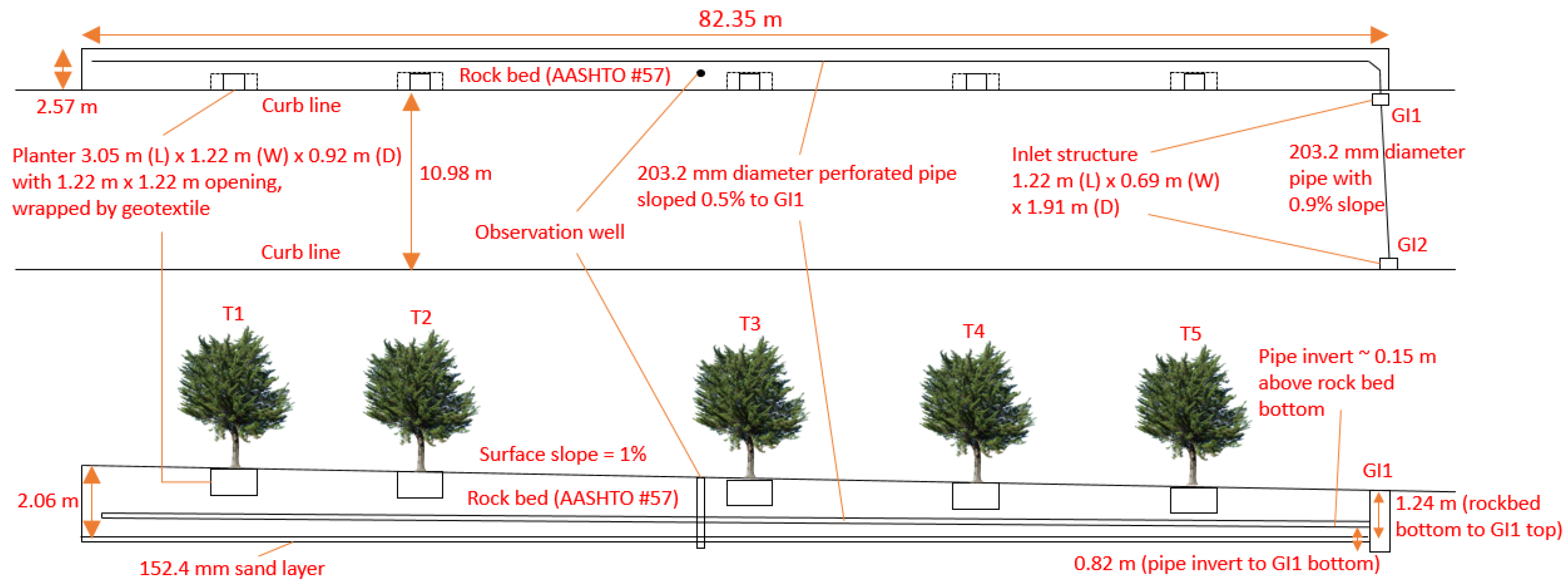
10]. Due to the limited building space in Philadelphia, many GIs have been built under sidewalks in the road right-of-way. For a typical tree trench GI built in Philadelphia, the runoff from the road surface enters an inlet structure, and a perforated distribution pipe transports and delivers water into the subsurface infiltration bed (i.e., a SCM), thus the flow direction is reversed from that of the application described earlier. Pretreatment is limited to a trash guard (a meshed filter bag) under the inlet grate or a sumped inlet due to space constraints.
Clogging analyses for similar systems are scarce. The hydraulic performance of similar systems has been investigated [11,12], but not the effects and characteristics of the clogging of an inflow distribution pipe as far as the authors could find. From the related field of drip irrigation, past studies have indicated that clogging is possible in similar systems [13], but the differences in pipe specifications and sources of water preclude a direct comparison. In addition to sediment, trash and/or leaves, stormwater runoff from road surfaces can be products from vehicle waste, atmospheric deposition, and road materials [14]. Since the characteristics of non-point pollution from stormwater runoff are complex [15], studies dedicated to the clogging of distribution pipes from untreated stormwater runoff are required.
Urbanization is a global trend. By 2010, more than 50% of the world’s population had moved into urban areas and such a population shift was achieved in the United States in the early 20th century [16]. As urban area expands, controlling non-point pollution from urban areas becomes more important as the impact to receiving water bodies from the complex human activities intensifies [17,18]. For such urban areas with limited building space, designs similar to the tree trench GI built in Philadelphia will play an important role in the future of urban stormwater management. Therefore, the purpose of this research is to understand the effects and characteristics of clogging and a cost-effective strategy in the maintenance of the distribution pipes of such systems.

2. Materials

2.1. Site Information

The SCM under investigation was constructed in 2013 in the northern suburban area of Philadelphia, Pennsylvania at approximately 40.07° N, 75.17° W (the sidewalk outside Hill Freedman World Academy). It is in the Cfa (humid subtropical) climate region according to the Koppen–Geiger climate classification system [19] with an average annual precipitation of 1054 mm from 1981 to 2010 [20]. Most monthly precipitation is distributed from 76 mm to 97 mm, with the exceptions of February as the driest month (66 mm) and July as the wettest month (109 mm). The average annual snowfall is 584 mm, which is typically from December to April with a peak in February.
As shown in Figure 1, this system is composed of five curbside planters, an underground rock infiltration bed in which the planters sit, two inlet structures (GI1 and GI2) collecting runoff from both sides of the street (with directly connected impervious drainage area of 2494 m2), and one distribution pipe delivering water collected by the inlet structures to the rock infiltration bed. The two inlet structures (GI1 and GI2 in the top section of Figure 1) are connected by a culvert with a diameter of 203.2 mm (sloped to GI1). Another perforated pipe with the same diameter (sloped to GI1) delivers water from the GI1 curb inlet structure to the rock bed (bottom section of Figure 1). Meshed trash guards (Figure 2) were installed in each inlet structure to reduce the amount of trash entering the distribution pipe. Inside the rock bed, the distribution pipe was uniformly perforated with an unspecified specification (personal communication with Philadelphia Water Department) and had an adverse 0.5% slope following the general design practice to bring debris towards the pipe entrance by gravity to facilitate maintenance cleaning. The only overflow points of the system were the street inlets GI1 and GI2, with GI1 located at a lower elevation. All dimensions were based on design drawings and post-construction invert measurements.
Instrumentation for this site included a weather station assemble comprising a Campbell CR800 data logger, a LI200X-L pyranometer (±3% typical error), a TE525 rain gage (±1% error) [21], a Hukseflux LP02-L25-P pyranometer (±10% error for daily sums) [22], and a Vaisala WXT520 multi-purpose weather station (±0.3 °C error for temperature, ±0.5 hPa for barometric pressure while temperature under 30 °C, ±3% for relative humidity less than 90%, ±3% for wind speed less than 35 m/s, ±3° for wind direction, and 5% for precipitation) [23], one HOBO [24] pressure transducer (±0.05% typical error) in each inlet structure (two total), an area-velocity sensor (±1 mm/s error for velocity and ±1 mm error for depth) with a ProSiren data logger [25] to measure the flow rate entering the distribution pipe at the entrance, a HOBO pressure transducer at the bottom of an observation well in the rock bed, and one set of soil moisture sensors [26] at various depths in each tree pit (five sets in total). All data had the same temporal interval of 5 min.

2.2. Observation

During the period from June 2016 to April 2018, periodic ponding in the inlet structure that submerged part of the distribution pipe entrance was observed during several field visits. Figure 3 shows a typical situation of such partial clogging. Collected water depth data of the GI1 inlet structure provided a more holistic view for periods of such partial clogging in Figure 4. The overflow depth of the inlet structure and the invert of the distribution pipe inlet are marked with black horizontal lines in Figure 4.
Figure 4 shows several long episodes of partial clogging as exhibited by continuous ponding above the invert of the pipe inlet (0.82 m) during the following range of dates: 25 February 2017–10 April 2017, 17 April 2017–5 May 2017, and after 31 January 2018. Ponding was also observed before 25 January 2017, but data collection was interrupted in winter 2016–2017, so the beginning of that partial clogging episode could not be determined. On 25 January 2017, a subsurface distribution pipe cleaning was performed, comprising of the injection of pressurized water jets into the distribution pipe and subsequent vacuuming. This was the only subsurface cleaning during the observation period from June 2016 to April 2018. Following the cleaning, the partial clogging situation was solved for a short period of time, but reconstituted during the storm on 25 February 2017. Note that all long partial clogging episodes happened in winter or spring.
In addition to those long episodes, several short episodes of partial clogging (e.g., 25 May 2017 and 19 June 2017) were also evident during summer. The data from 25 May 2017 contained two events with the first event being free from and the second exhibiting significant partial clogging, as shown in Figure 5. Rainfall associated with the two storms was separated by more than six hours, so they were considered as two distinct storms. After the first peak of the second storm, the water depth recession rate in the GI1 inlet structure after cessation of rainfall reduced significantly when compared to that of the first storm, showing partial clogging of the distribution pipe. For all storms, the water level in the rock bed was always lower than that in the inlet structure, as shown in Figure 5. In Figure 5, the bottom of the inlet structure was the datum for all water depths or elevations. As the bottom of the rock bed is higher than that of the inlet structure, the water depth in the rock bed showed a flat line when dry.
One phenomenon that was not explained in both Figure 4 and Figure 5 was the low water depth in the inlet structure at the final balance state for periods without partial clogging. It was around 0.6 m from the bottom and significantly lower than the invert of the distribution pipe inlet (0.82 m), which could only have been caused by a leaking inlet structure. The leaking rate varied significantly. For example, based on the water depth recession rate from the invert of the pipe inlet (0.82 m) to the final depth (0.6 m), Figure 5 shows a much faster leaking rate for the first storm than that for the second storm. As excavation of the site was not possible, it could only be hypothesized as the result of the variation of soil moisture and groundwater level in the surrounding soil. Nevertheless, the leaking rate was very small at about 8 × 10⁻⁶ m3/s (based on the first storm of Figure 5) or less, so its effect could be ignored. Water recession was accelerated below the pipe invert in Figure 5 as the water surface area above the pipe invert (i.e., including water in the pipe) would be much larger than that between the invert of the pipe inlet and the leaking point (i.e., only water in the inlet structure). The leaking point in the inlet structure was located during the subsurface pipe cleaning on 25 January 2017 when the inlet structure was pumped dry, shown as the small stream of water circled by the red oval in Figure 6. In Figure 6, water flowed back into the inlet structure, which can only be explained by the saturated condition of the surrounding soil caused by the high ponding situation before 25 January 2017.
The observations based on field visits and collected data showed a complicated nature of partial clogging of the distribution pipe. Despite a few short episodes in summer, most partial clogging episodes were clustered in winter. The effect of undersurface pipe cleaning was short lived in winter, but most of the partial clogging situations were mitigated by itself in summer without human intervention. Even though such partial clogging did not appear to increase the tendency of overflow (only the short episode on 19 June 2017 had overflow), how such partial clogging affected the performance of the distribution pipe should be understood. If an impact on the distribution pipe performance did exist, the patterns of its influence (i.e., uniform influence across all storms, or higher influence towards small/large storms) should be evaluated in order to decide on a maintenance strategy against such partial clogging, and to avoid the loss of system performance during large storms.

3. Methods

Ongoing research determined that the flow rate sustained by the distribution pipe was limited by the orifices on the pipe wall, so the following analyses were based on the orifice flow equation. Assuming that the partial clogging blocked a portion of the orifice area, the orifice equation for a single orifice can be rewritten as Equation (1). In Equation (1), q is the orifice flow rate, ϵ is the portion (ranging from 0 to 1) of the orifice area that is functional, C is the orifice discharge coefficient, a is the orifice area before partial clogging happens, g is the gravity constant (9.8 m/s2), and h d is the pressure head driving the orifice flow (called “driving head” hereafter).
q = C ( ϵ a ) 2 g h d
Equation (1) can be rearranged for ϵ in Equation (2).
ϵ = q C a 2 g h d = q ( C 2 g ) ( a h d ) q a h d
In Equation (2), C and g can be considered constants, so ϵ is linearly proportional to q a h d . The authors decided to assume the discharge coefficient C as a constant, based on the fact that the discharge coefficient C for parallel flow (i.e., flow in the pipe is parallel to the plane of the orifice) was in a narrow range of 0.61–0.64 [27].
For orifices uniformly distributed on a section of perforated pipe, Equation (2) can be rewritten as Equation (3), where Ε is the mean portion of clogging on the section of pipe, Q is the sum of the orifice flow generated by the section of pipe, A is the total orifice area on that section of pipe, n is the number of orifices on the section of pipe, h d , i represents the driving head at the i-th orifice, and h d , m e a n represents the mean driving head among all orifices on the section of pipe. The approximation performed in Equation (3) delivered a low approximation error after being tested by actual examples of a numerical series. The goal of the derivation was only to provide a means to compare the relative magnitudes of partial clogging among different events.
Ε Q A i = 1 n h d , i n Q A ( i = 1 n h d , i n ) = Q A h d , m e a n
Since the orifices are uniformly distributed on the perforated pipe, the total orifice area on the section of pipe is linearly proportional to the length of the pipe which allows orifice flow; therefore, performance index i (Equation (4)) can be derived to represent the performance of the perforated pipe based on Equation (3), with higher values representing less influence from partial clogging (i.e., higher performance).
i = Q l e f f h d , m e a n
where l e f f is the effective length of distribution pipe that allows orifice flow, which is the equivalent length of water column with the same volume of water (V) in the pipe and the cross-sectional area (A) of the pipe, as explained by Equation (5).
l e f f = V A
Detailed definitions of parameters (for h d , m e a n and l e f f ) for the performance index under various scenarios are discussed below. 
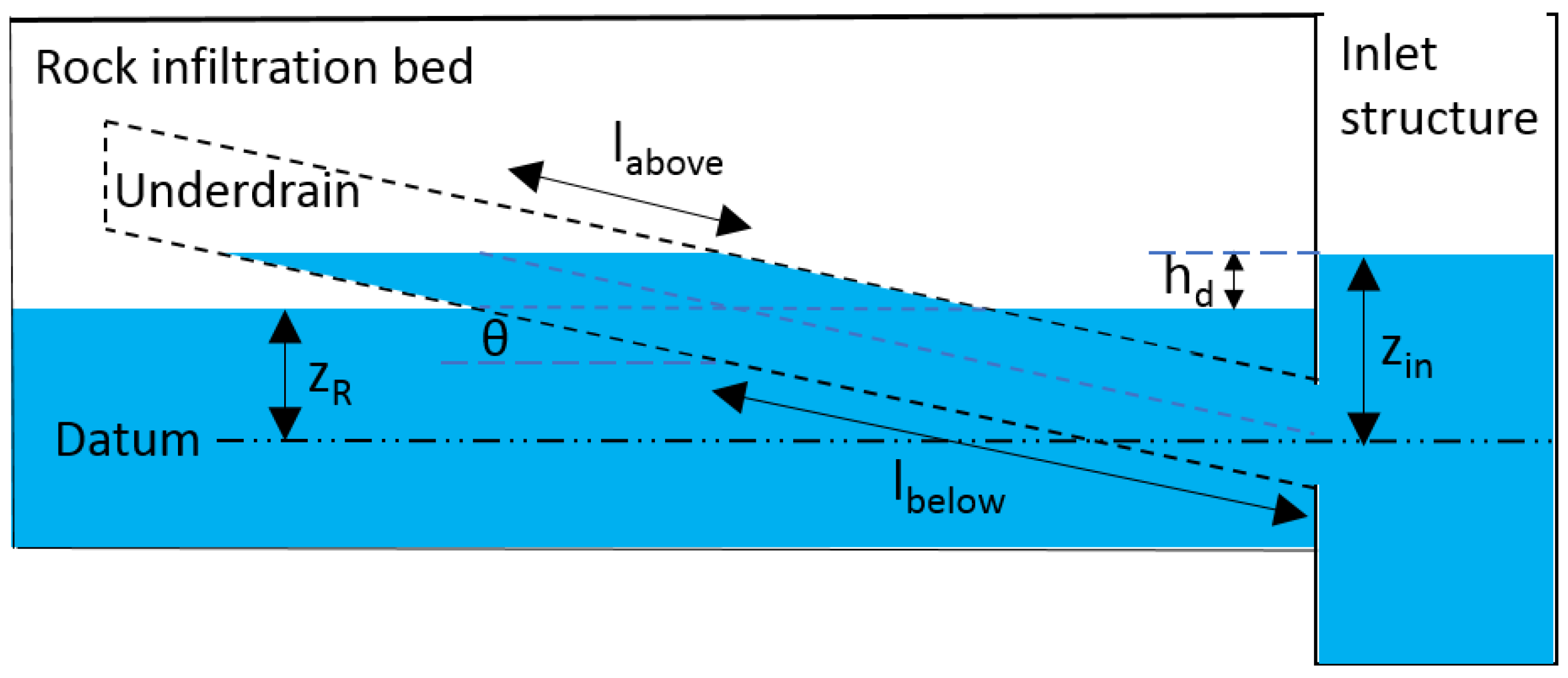
Figure 7 describes the operation of a typical distribution system. The datum was set at the elevation of the center of the distribution pipe at its inlet. Water elevation in the rock bed and in the inlet structure were z R and z i n , respectively, with difference h d . Along the centerline of the pipe (with inclination angle θ ), the length of water (along the pipe centerline) above and below the water in the rock bed (elevation z R ) was l a b o v e ( h d ) and l b e l o w ( z R ), respectively. For the condition considered by Figure 7, z R and z i n were both lower than the top of the distribution pipe. Other conditions were analyzed as provided below.
From the recorded data, the water surface inside the distribution pipe and that in the inlet structure were very close to each other in elevation as the difference of the velocity head was proven to be negligible. This implied that the driving head was the water surface elevation difference h d . The driving head was constant anywhere below the rock bed water surface z R . The driving head above z R was simply the hydrostatic pressure of the water column above z R , with zero at the top of the water column and linearly increasing to h d at the elevation of z R . The mean driving head ( h d ,   m e a n ) acting on the pipe can thus be derived in Equation (6) below.
h d , m e a n ( h d 2 l a b o v e + h d l b e l o w ) ( l a b o v e + l b e l o w ) = [ h d 2 ( h d csc ( θ ) ) + h d ( z R csc ( θ ) ) ] ( z i n csc ( θ ) ) = ( h d 2 2 + h d z R ) z i n
The effective pipe length was simply provided by Equation (7):
l e f f z i n csc ( θ )
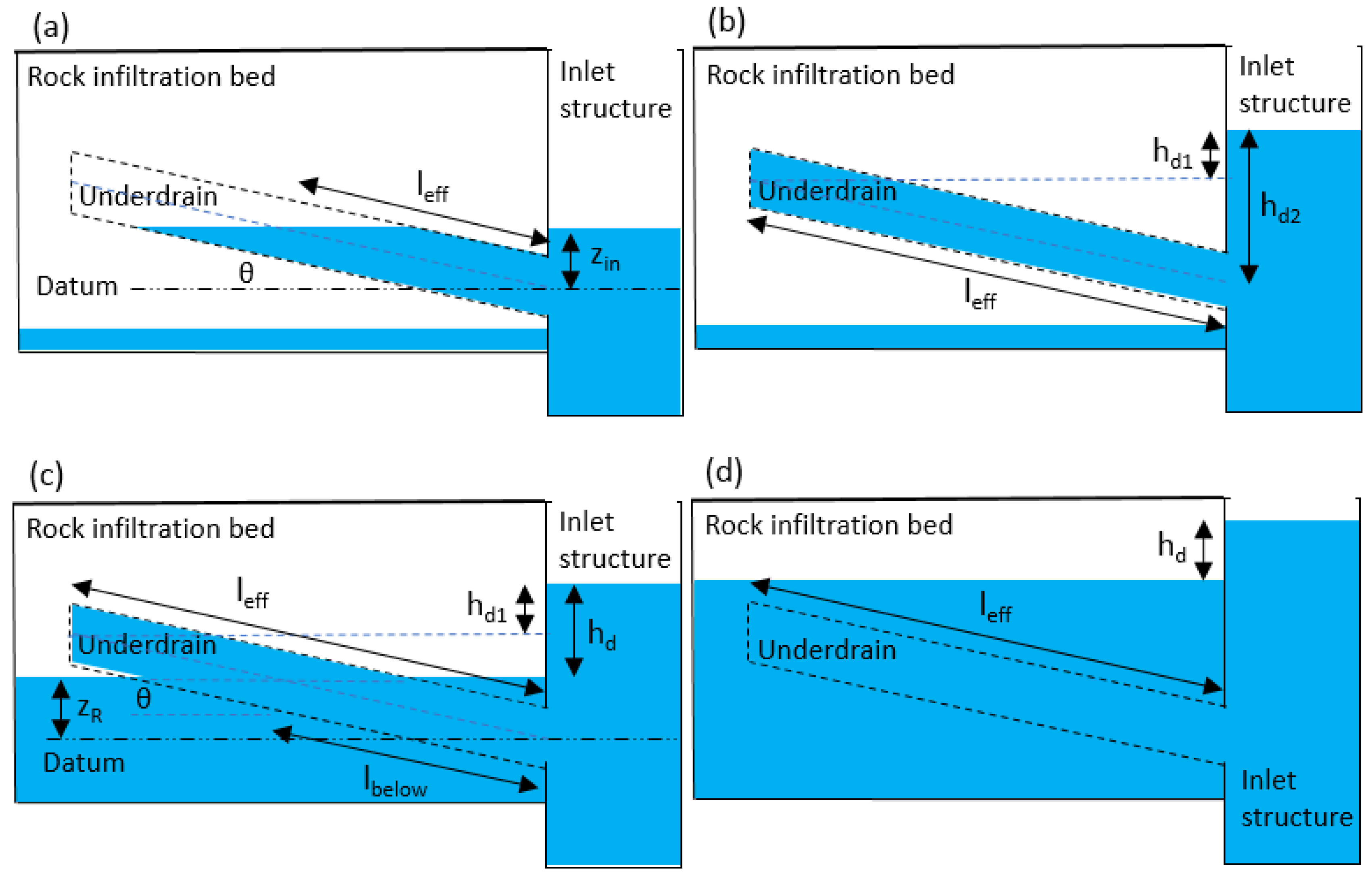
Other than the condition depicted in Figure 7, four other possible conditions were analyzed as illustrated in Figure 8. All items in Figure 8 were defined previously, except for h d 1 and h d 2 , which indicates the distance from the water surface in the inlet structure to the top and the inlet of the distribution pipe (along its centerline) in Figure 8b, respectively. Note that conditions with either z R or z i n below the top of the distribution pipe inlet were excluded from consideration as the effective length of water in the pipe of such conditions cannot be based on the pipe length with a fully wetted perimeter like that of the other considered conditions.
Analyses based on Figure 8a were similar to those done for the water column above z R in Figure 7, with the mean driving head and the effective pipe length calculated by Equations (8) and (9) below:
h d , m e a n z i n 2
l e f f z i n csc ( θ )
Intense storms created conditions depicted by Figure 8b–d, where the water elevation in the inlet structure builds up quickly. The distribution pipe was completely full, but water in the rock infiltration bed can still be relatively shallow. Similar to Equation (8), the mean driving head for Figure 8b was provided by Equation (10) below, and the effective pipe length l e f f is simply the length of the whole pipe.
h d , m e a n h d 1 + h d 2 2
Figure 8c has a form similar to that of Figure 7 with the mean driving head for Figure 8c provided by Equation (11) below, while the effective pipe length ( l e f f ) is the length of the whole pipe ( l p i p e ).
h d , m e a n ( ( h d + h d 1 2 ) ( l p i p e l b e l o w ) + h d l b e l o w ) l p i p e
where l b e l o w is the length of pipe under z R and is given by l b e l o w z R csc ( θ ) .
The last condition (Figure 8d) had a constant driving head throughout the distribution pipe because the whole pipe was submerged, thus h d , m e a n = h d , and the effective pipe length l e f f is the length of the whole pipe l p i p e .

4. Results

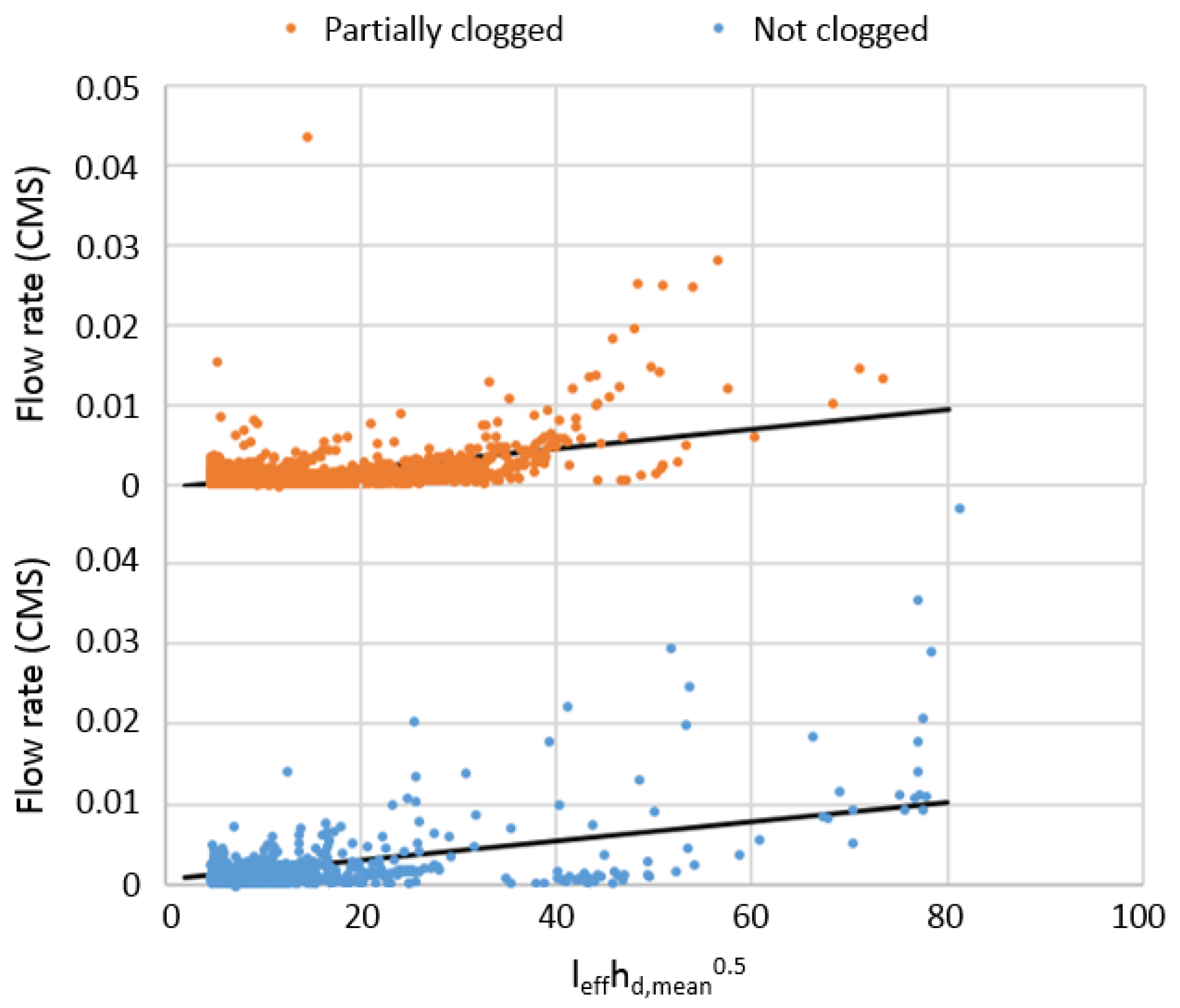
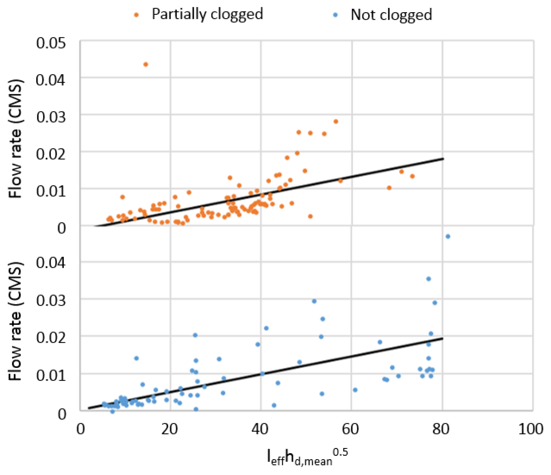
Variations of orifice performance can be examined by plotting the measured flow rate against l e f f h d , m e a n , as shown by Figure 9 with the data with zero flow excluded. All data from November 2016 to April 2018 was utilized in Figure 9. According to Equation (4), the flow rate Q divided by l e f f h d , m e a n in Figure 9 represents performance. The dates of partial clogging and no clogging were determined from Figure 4. Thick black lines in Figure 9 represent the linear regression lines generated through ANCOVA, as discussed below.
l e f f h d , m e a n appeared to be a strong predictor for flow rate with p < 0.0001 for both the non-clogging and partial clogging data. ANCOVA (ANalysis of COVAriance) was utilized to examine the effect of partial clogging on the distribution of the pipe performance. Similar to the popular ANOVA (ANalysis Of VAriance), ANCOVA tests the null hypothesis that two population means are equal, but ANCOVA considers the effect of a “covariate”, which is likely to be correlated with the dependent variable [28]. Such a covariate was coded as one dummy variable of either 0 (represents no clogging) or 1 (represents partial clogging) in the linear regressions in this research. The shift of linear regression lines due to the covariate in Figure 9 between periods with and without clogging appeared to be small through visual inspections, but statistical analyses by ANCOVA showed strong evidence (p < 0.0001) that partial clogging, on average, had an impact on performance.
The above ANCOVA result was based on all data, with a large portion of the data from periods with very slow drawdown of water level in the inlet structure after the storms ended, as illustrated in Figure 5. As the focus of this research was on how partial clogging can affect orifice performance during larger storm events (when overflow occurs), the results from periods with slow drawdown and lower rainfall intensities were of less interest. Table 1 provides the ANCOVA results with the different rainfall intensity criteria below which shows which data entries were excluded. The p-value showing no difference in performance between no clogging and partial clogging were in bold.
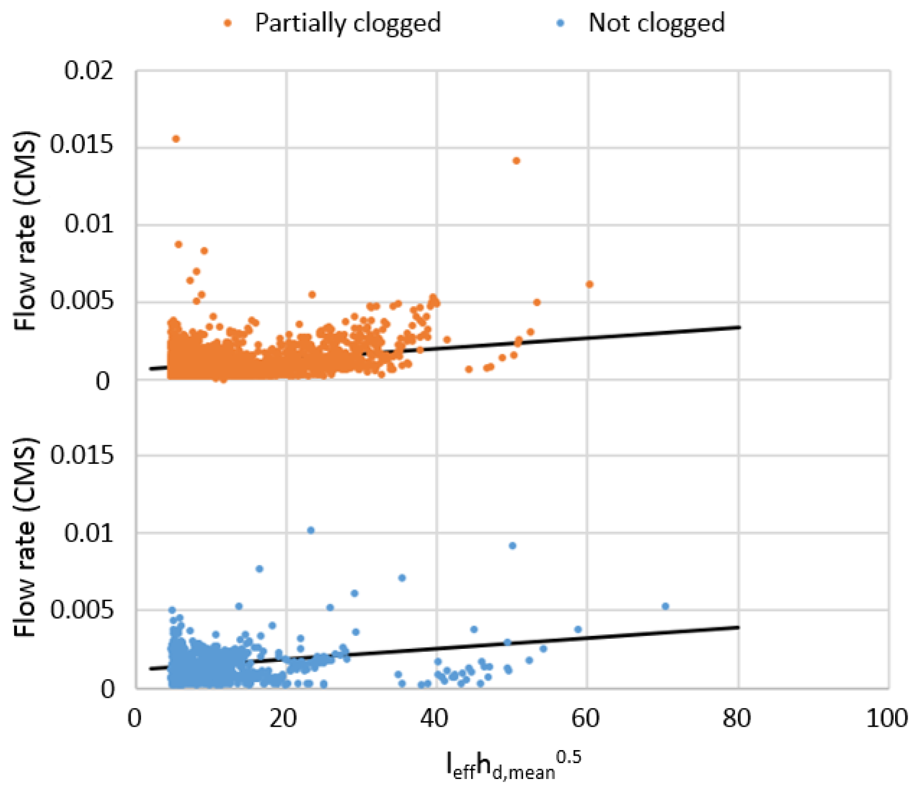
Table 1 shows that even though partial clogging had a significant effect during dry periods or low-intensity storms, its effect declines as the storm intensity increases. When rainfall intensity was higher than approximately 0.65 mm/5 min, the effect of partial clogging was not statistically distinguishable, and thus did not impact system performance. The distribution of data with a rainfall intensity criterion of 0.65 mm/5 min is provided in Figure 10, while the distribution of data with a rainfall intensity lower than the criterion was provided in Figure 11 for comparison. Thick black lines represent the linear regression lines generated through ANCOVA. Please note that the scale on the y-axis in Figure 11 is different from that of Figure 9 or Figure 11. Again, the shift of linear regression lines due to the covariate of clogging appeared to be small in both figures through visual inspection; however, statistical analyses by ANCOVA provided clear evidence that the effects of clogging could not be distinguished (p = 0.152, Table 1) in Figure 10 but were significant (p < 0.0001) in Figure 11.

5. Discussion

First, the drawdown data of the infiltration bed were examined. The relation between water depth and drawdown rate exhibited little variation throughout the observation period, thus showing no clogging of the infiltration bed. Therefore, the infiltration bed had no influence in explaining the results from the above analyses.
Second, the Froude number was examined. It was determined that 99.89% of non-zero flow during storms was in the subcritical state; therefore, the effect from switching between subcritical and supercritical states could be ignored.
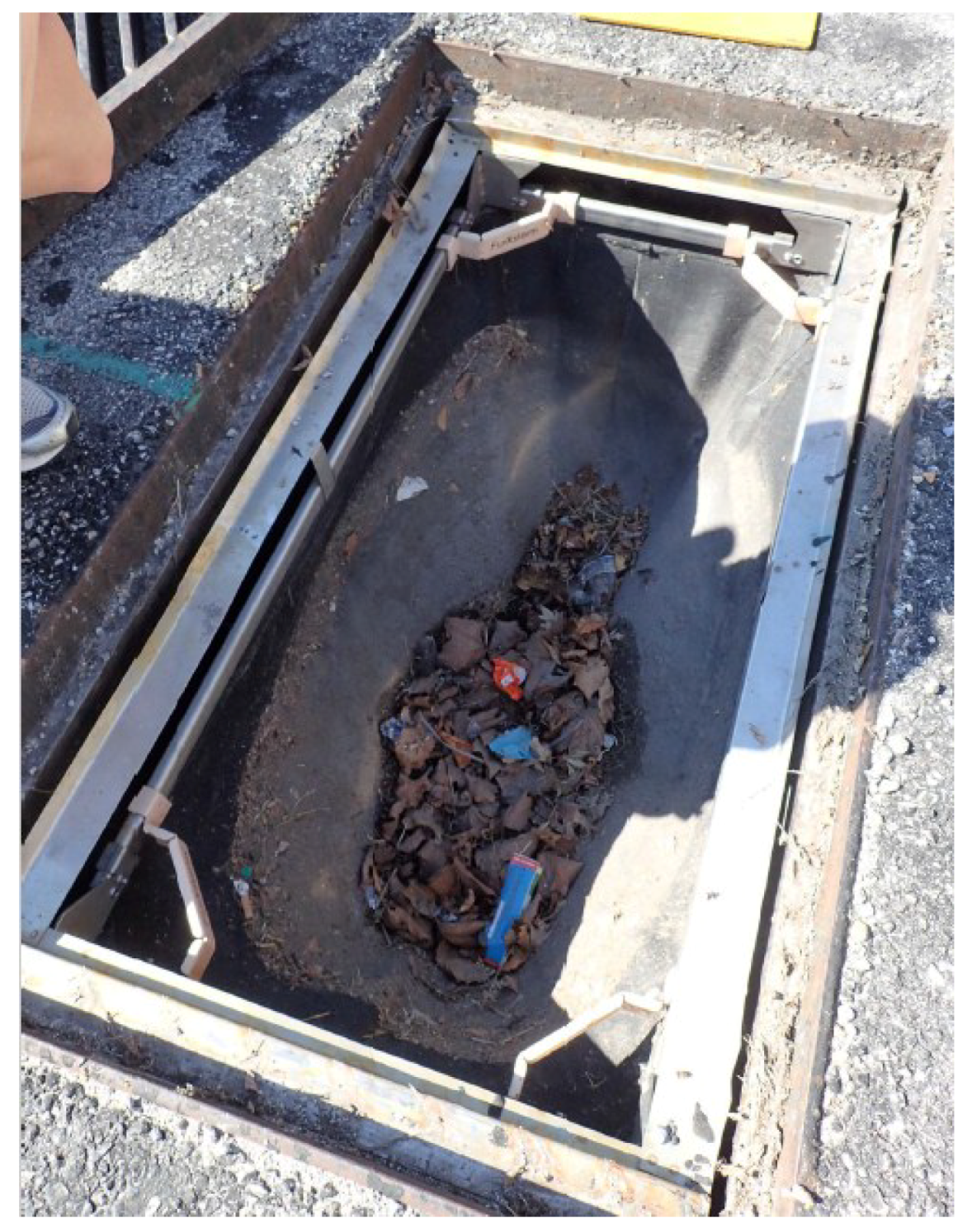
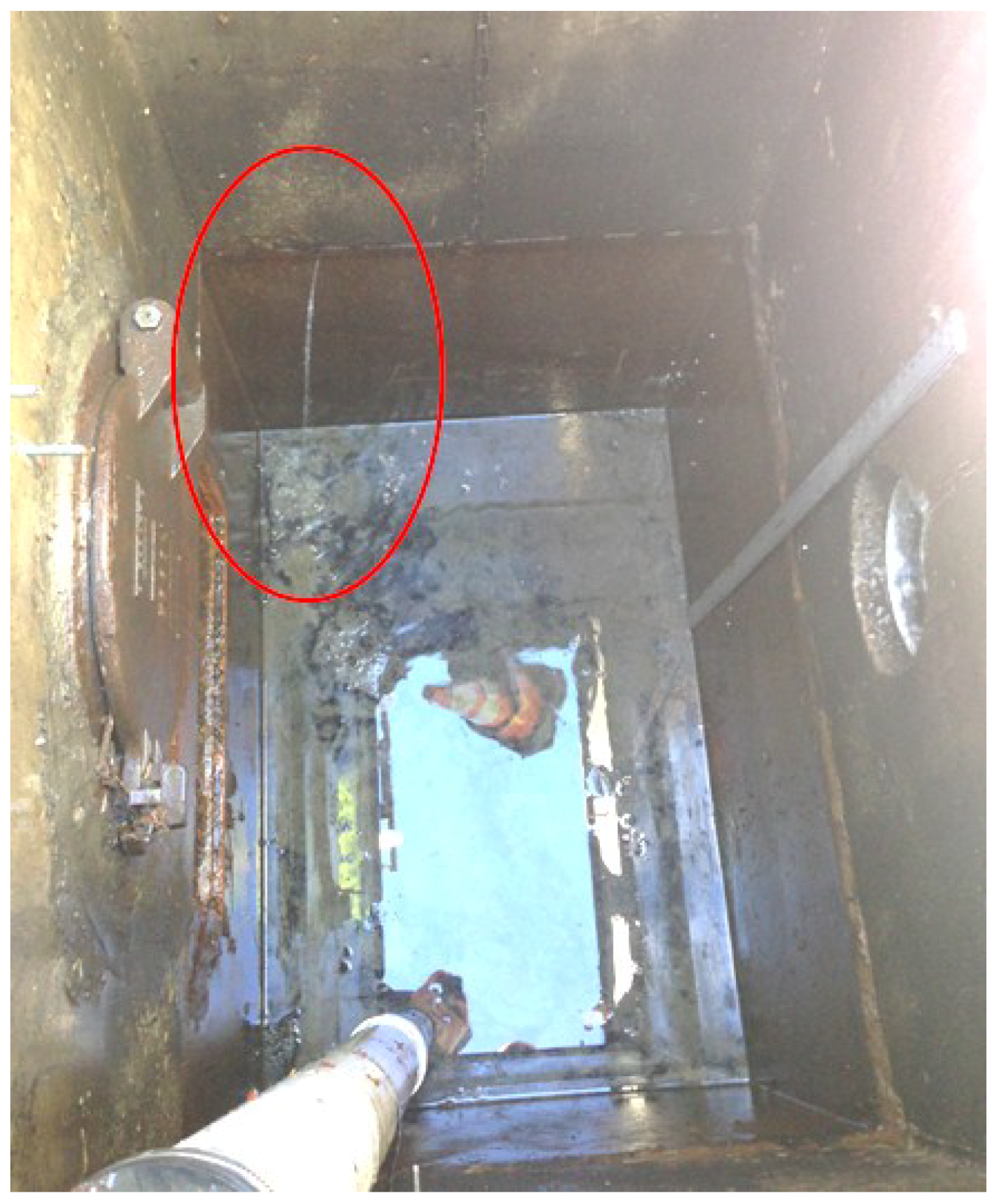
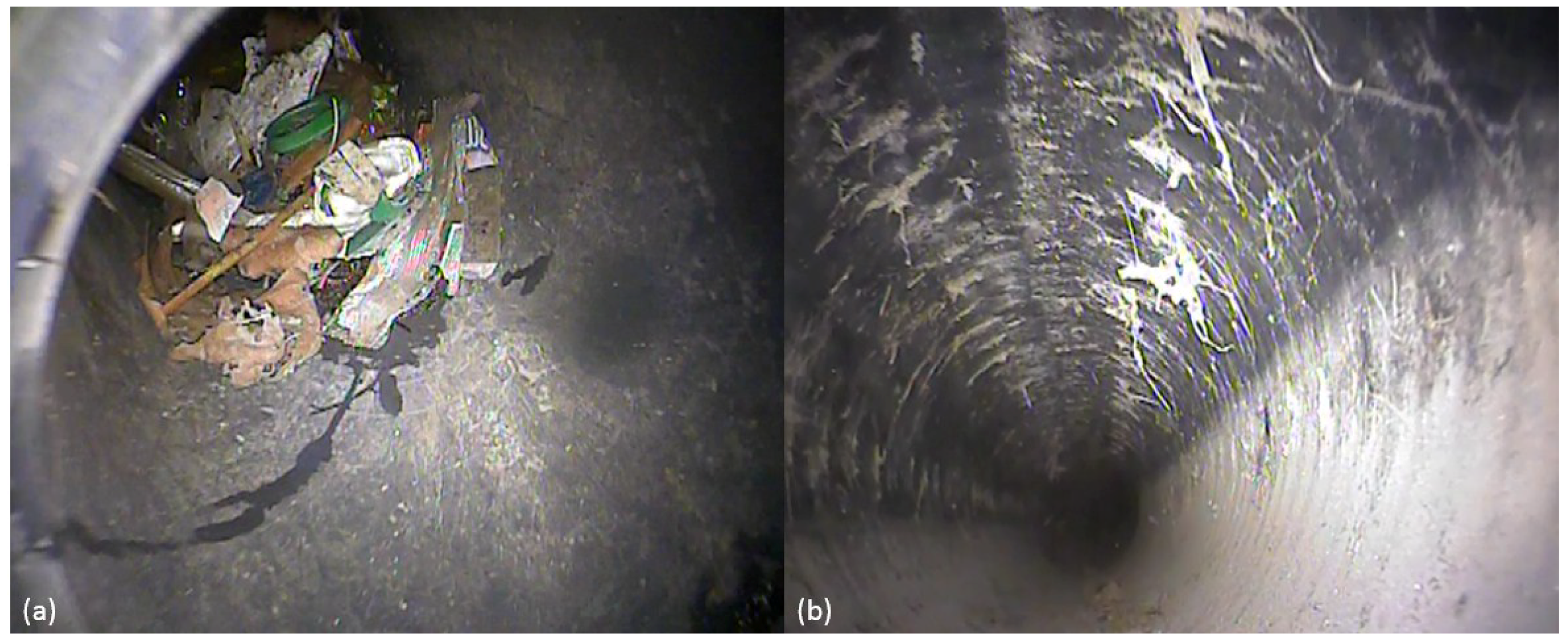
The records of subsurface maintenance done in the past were then examined to explain the results from the analyses. The archived video observation (20 June 2016) showed a significant quantity of debris deposited close to the 90-degree turn of the pipe near the entrance, as shown in Figure 12a. After passing the debris pile, the distribution pipe was generally clean, as Figure 12b shows. Another subsurface maintenance performed on 25 January 2017 found more debris, and the debris was piled mostly in the lower (i.e., close to the inlet) 30 m of the pipe. The spatially uneven distribution of debris might be explained by the reversed slope of the distribution pipe that would bring most debris back to the entrance.
Since most debris was accumulated near the lowest point of the distribution pipe, it appeared to cause partial clogging as water lower than the elevation of the debris cannot enter the rock infiltration bed through the orifices at the bottom section of the pipe. However, during storm events, the incoming water either moved the debris block, thus exposing the orifices, or overtopped the debris block thus accessing the remaining distribution pipe. Such moving of debris can cause the partial clogging to break temporarily (e.g., 10 April 2017–17 April 2017) as observed in Figure 4.
In Figure 12a, it was visible that a significant portion of debris appeared to be leaves and paper with only a small portion being plastic, even though a trash guard had been installed in the inlet structure to minimize the amount of leaves entering the inlet structure with runoff. Due to the ample supply of fallen leaves in late autumn in Philadelphia, the debris pile would potentially continue to grow in winter if the leaves can get past the trash guard.
As the supply of leaves is ample in winter and most winter storms are low in both depth and intensity, the clogging effect was significant in winter. As larger storms appeared in summer, the leaves and debris could be pushed into the higher end of the pipe, thus exposing the orifices. No subsurface cleaning was performed after January 2017 in the observation period; therefore, such mechanisms can sustain the pipe performance (during larger storms) for at least a full year. In any event, scheduled cleaning of the distribution pipe is recommended to reduce the amount of accumulated debris as the debris does not disappear completely and could still cause short episodes of partial clogging during the summer. If left unchecked, the accumulated debris may block the distribution pipe and cause a significant drop in system performance.

6. Conclusions

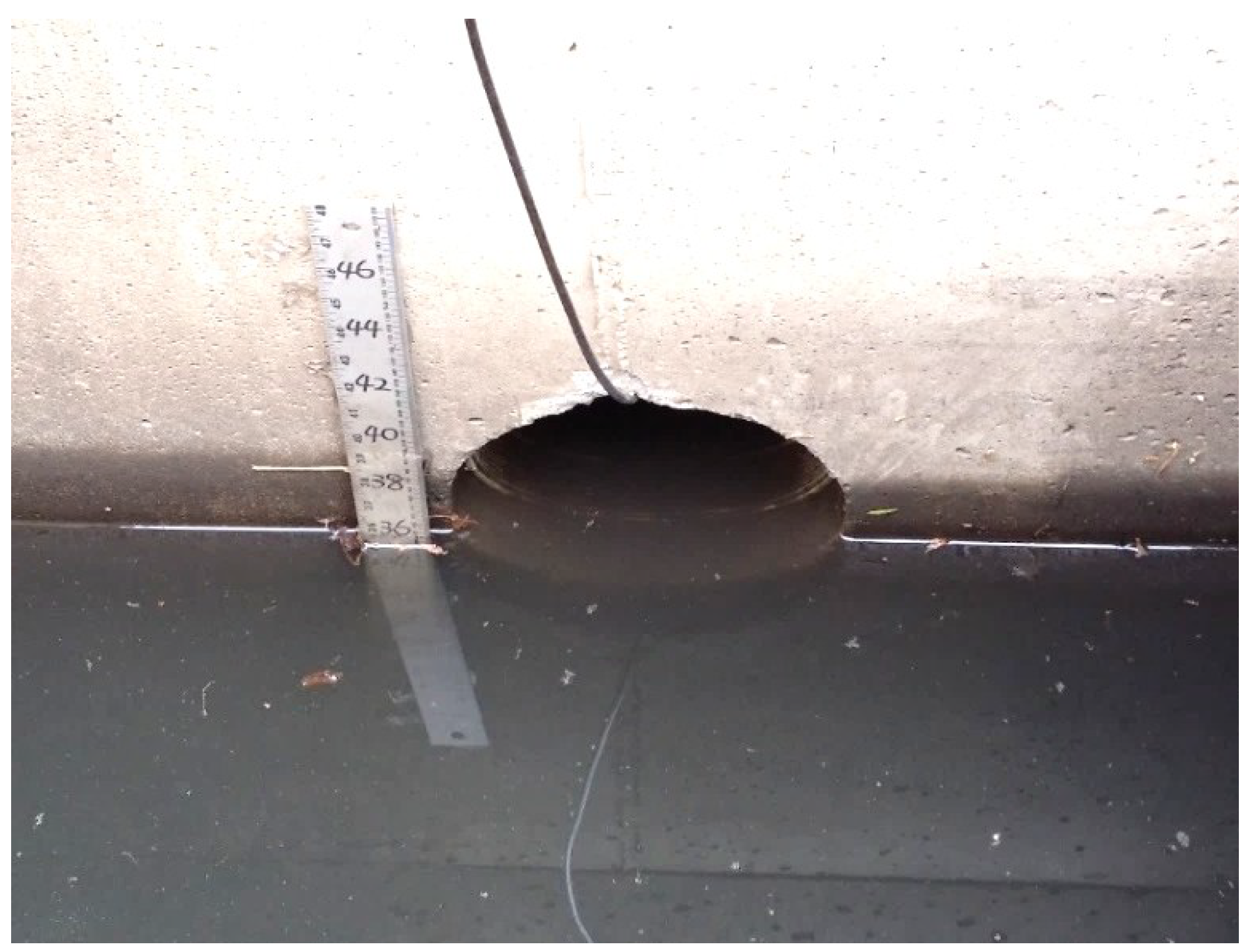
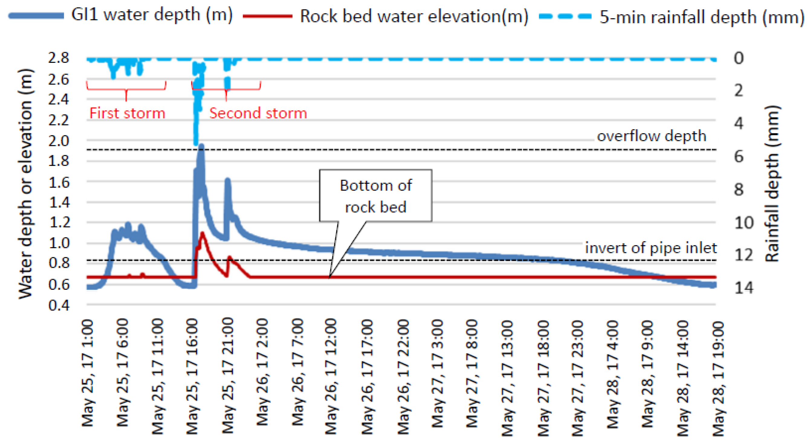
Partial clogging of a distribution pipe system was found by both visual observations and data analyses as evidenced by continuous ponding in the inlet structure, partially submerging the entrance of the distribution pipe. The impact on orifice performance of the distribution pipe from such partial clogging was examined by plotting the flow rate vs. l e f f h d , m e a n where h d , m e a n is the mean driving head and l e f f the effective pipe length. ANCOVA was used to determine the impact of partial clogging on orifice performance of the distribution pipe. Although partial clogging was found to exhibit a statistically significant effect on pipe performance, its effect declined with higher rainfall intensity, and was eventually not distinguishable when rainfall intensity was higher than approximately 0.65 mm/5 min. From ongoing research, the system overflowed only when the rainfall intensity was higher than approximately 3.3 mm/5 min. Therefore, partial clogging did not have any detrimental effect on the overflow generating characteristics of this system.
The subsurface maintenance records showed that most debris was piled up near the lower portion of the distribution pipe, which caused the observed partial clogging. However, the incoming water during larger storms (rainfall intensity higher than approximately 0.65 mm/5 min) either moved the debris block thus exposing the orifices, or overtopped the debris block thus accessing the remaining distribution pipe, so the performance of the distribution system during larger storms was not affected. It was hypothesized that most debris was composed of leaves, which are in abundant supply during late fall and early winter in Philadelphia. This explained why the occurrence of partial clogging was most frequent in winter.
Partial clogging was difficult to completely eliminate even with the installation of a trash guard and cleaning of the distribution pipe (the first clogging happened only one month after cleaning in January 2017). For drainage systems with space limitations such as the system under examination by this research, effective pretreatment is often not an option. Therefore, it poses a question to maintenance staff and practitioners—do we need to multiply the maintenance cost to eliminate all observed partial clogging? The result of this research implied that it is not necessary to increase the cleaning frequency to eliminate all partial clogging. In Philadelphia or locations with similar climate and flora, a typical trash guard and regular (once to twice per year) pipe cleaning was sufficient to keep the distribution pipe system at a satisfactory performance. Typical partial clogging does not harm the system performance during storms, when sufficient pipe delivery performance is needed the most.
However, such guidelines are qualitative, and more specific quantitative directives are required. For future research, two directions are suggested on this topic:
  • Find the minimal maintenance schedule needed to maintain the performance, and
  • Find the relations between the distribution pipe specification, pipe diameter, orifice size, orifice density), and the minimal needed maintenance schedule, so that a balance between construction cost and maintenance cost can be found.

Author Contributions

Conceptualization, M.-C.T.; Methodology, M.-C.T.; Software, M.-C.T.; Validation, M.-C.T.; Formal Analysis, M.-C.T.; Investigation, M.-C.T. and R.T.; Resources, R.T.; Data Curation, M.-C.T.; Writing-Original Draft Preparation, M.-C.T.; Writing-Review & Editing, R.T.; Visualization, M.-C.T.; Supervision, R.T.; Project Administration, R.T.; Funding Acquisition, R.T.

Funding

This publication was developed under Assistance Agreement No. 83555601 awarded by the U.S. Environmental Protection Agency to Villanova University. It has not been formally reviewed by the EPA. The views expressed in this document are solely those of Villanova University and do not necessarily reflect those of the Agency. The EPA does not endorse any of the products or commercial services mentioned in this publication.

Acknowledgments

The support from Philadelphia Water Department was crucially important for the success of this study and is highly appreciated, particularly the assistance from Stephen White and Chris Bergerson. The assistance from Cara Albright who designed and set up all instrumentation is also noted and highly appreciated.

Conflicts of Interest

The authors declare no conflicts of interest.

References

  1. Davis, A.P.; Hunt, W.F.; Traver, R.G.; Clar, M. Bioretention Technology: Overview of Current Practice and Future Needs. J. Environ. Eng. 2009, 135, 109–117. [Google Scholar] [CrossRef]
  2. Siriwardene, N.R.; Deletic, A.; Fletcher, T.D. Clogging of Stormwater Gravel Infiltration Systems and Filters: Insights from a Laboratory Study. Water Res. 2007, 41, 1433–1440. [Google Scholar] [CrossRef] [PubMed]
  3. Le Coustumer, S.; Fletcher, T.D.; Deletic, A.; Barraud, S.; Poelsma, P. The Influence of Design Parameters on Clogging of Stormwater Biofilters: A Large-Scale Column Study. Water Res. 2012, 46, 6743–6752. [Google Scholar] [CrossRef] [PubMed]
  4. Kandra, H.S.; McCarthy, D.; Fletcher, T.D.; Deletic, A. Assessment of Clogging Phenomena in Granular Filter Media Used for Stormwater Treatment. J. Hydrol. 2014, 512, 518–527. [Google Scholar] [CrossRef]
  5. Pezzaniti, D.; Beecham, S.; Kandasamy, J. Influence of Clogging on the Effective Life of Permeable Pavements. Water Manag. 2009, 162, 211–220. [Google Scholar] [CrossRef]
  6. Lucke, T.; Beecham, S. Field Investigation of Clogging in A Permeable Pavement System. Build. Res. Inform. 2011, 39, 603–615. [Google Scholar] [CrossRef]
  7. Larrahondo, J.M.; Atalay, F.; McGillivray, A.V.; Mayne, P.W. Evaluation of Road Subsurface Drain Performance by Geophysical Methods. In Proceedings of the GeoCongress 2008: Geosustainability and Geohazard Mitigation, New Orleans, LA, USA, 9–12 March 2008. [Google Scholar]
  8. Payne, E.; Hatt, B.; Deletic, A.; Dobbie, M.; McCarthy, D.; Chandrasena, G. Adoption Guidelines for Stormwater Biofiltration Systems—Summary Report; Cooperative Research Centre for Water Sensitive Cities: Clayton, Australia, 2015. [Google Scholar]
  9. Davis, A.P.; Traver, R.G.; Hunt, W.F.; Lee, R. Hydrologic Performance of Bioretention Storm-Water Control Measures. J. Hydrol. Eng. 2012, 17, 604–614. [Google Scholar] [CrossRef]
  10. Green City, Clean Waters. Available online: http://www.phillywatersheds.org/what_were_doing/documents_and_data/cso_long_term_control_plan (accessed on 6 April 2018).
  11. Murphy, P.; Kaye, N.B.; Khan, A.A. Hydraulic Performance of Aggregate Beds with Perforated Pipe Underdrains Flowing Full. J. Irrig. Drain. Eng. 2014, 140, 04014023. [Google Scholar] [CrossRef]
  12. Afrin, T.; Khan, A.A.; Kaye, N.B.; Testik, F.Y. Numerical Model for the Hydraulic Performance of Perforated Pipe Underdrains Surrounded by Loose Aggregate. J. Hydraul. Eng. 2016, 142, 04016018. [Google Scholar] [CrossRef]
  13. Ravina, I.; Paz, E.; Sofer, Z.; Marcu, A.; Shisha, A.; Sagi, G. Control of Emitter Clogging in Drip Irrigation with Reclaimed Wastewater. Irrig. Sci. 1992, 13, 129–139. [Google Scholar] [CrossRef]
  14. Li, M.-H.; Barrett, M.E. Relationship Between Antecedent Dry Period and Highway Pollutant: Conceptual Models of Buildup and Removal Processes. Water Environ. Res. 2008, 80, 740–747. [Google Scholar] [CrossRef] [PubMed] [Green Version]
  15. Lee, J.H.; Bang, K.W. Characterization of Urban Stormwater Runoff. Water Res. 2000, 34, 1773–1780. [Google Scholar] [CrossRef]
  16. Grimm, N.B.; Faeth, S.H.; Golubiewski, N.E.; Redman, C.L.; Wu, J.; Bai, X.; Briggs, J.M. Global Change and The Ecology of Cities. Science 2008, 319, 756–760. [Google Scholar] [CrossRef] [PubMed]
  17. Tu, M.-C.; Smith, P. Modelling Pollutant Buildup and Washoff Parameters for SWMM Based on Land Use in a Semiarid Urban Watershed. Water Air Soil Pollut. 2018, 229, 121. [Google Scholar] [CrossRef]
  18. Tu, M.-C.; Smith, P.; Filippi, A.M. Hybrid Forward-selection Method-based Water-quality Estimation via Combining Landsat TM, ETM+, and OLI/TIRS Images and Ancillary Environmental Data. PLoS ONE 2018. [Google Scholar] [CrossRef] [PubMed]
  19. Peel, M.C.; Finlayson, B.L.; McMahon, T.A. Updated World Map of the Koppen-Geiger Climate Classification. Hydrol. Earth Syst. Sci. 2007, 11, 1633–1644. [Google Scholar] [CrossRef]
  20. Climate Data Online. Available online: https://www.ncdc.noaa.gov/cdo-web/ (accessed on 6 April 2018).
  21. Products. Available online: https://www.campbellsci.com/products (accessed on 6 April 2018).
  22. Pyranometers & Solar Radiometers. Available online: http://www.huksefluxusa.com/products-services/solar-radiometers-pyranometers/ (accessed on 6 April 2018).
  23. User’s Guide: Vaisala Weather Transmitter WXT520. Available online: https://www.vaisala.com/sites/default/files/documents/M210906EN-C.pdf (accessed on 6 April 2018).
  24. Featured Products. Available online: http://www.onsetcomp.com/ (accessed on 6 April 2018).
  25. Cloud Enabled Wireless Data Monitoring Systems. Available online: http://www.blue-siren.com/ (accessed on 6 April 2018).
  26. Soil Sensors. Available online: http://www.stevenswater.com/products/sensors/soil/ (accessed on 6 April 2018).
  27. Bailey, B.J. Fluid Flow in Perforated Pipes. J. Mech. Eng. Sci. 1975, 17, 338–347. [Google Scholar] [CrossRef]
  28. Huitema, B. The Analysis of Covariance and Alternatives, 2nd ed.; John Wiley & Sons: Hoboken, NJ, USA, 2011. [Google Scholar]
Figure 1. Plan view (top) and profile view (bottom) of the site under investigation.
Water 10 01045 g001
Figure 2. Trash guard installed in the GI1 inlet structure (Date: 18 October 2016).
Water 10 01045 g002
Figure 3. Ponding in the inlet structure due to partial clogging of the distribution pipe (Date: 30 March 2017).
Water 10 01045 g003
Figure 4. Water elevation in the GI1 inlet structure between June 2016 and April 2018.
Water 10 01045 g004
Figure 5. Rainfall depth and water depth (inlet structure and rock bed, with the bottom of the inlet structure as the datum) from events without (first storm) and with (second storm) partial clogging on 25 May 2017.
Water 10 01045 g005
Figure 6. Leaking point in the inlet structure (Date: 25 January 2017).
Water 10 01045 g006
Figure 7. Profile view of a typical distribution system in this research.
Water 10 01045 g007
Figure 8. Conditions considered in the pipe performance determination in addition to the condition of Figure 7. (a) Water in the rock bed is lower than the whole pipe and the pipe is half-full; (b) water in the rock bed is lower than the whole pipe and the pipe is full; (c) water in the rock bed is between the lower and higher ends of pipe, and the pipe is full; (d) water in the rock bed submerges the whole pipe.
Water 10 01045 g008
Figure 9. Performance plotted as flow rate vs. h d , m e a n l e f f for all data.
Water 10 01045 g009
Figure 10. Performance plotted as flow rate vs. h d , m e a n l e f f for all data with 5-min rainfall depth >0.65 mm.
Water 10 01045 g010
Figure 11. Performance plotted as flow rate vs. h d , m e a n l e f f for all data with 5-min rainfall depth <0.65 mm.
Water 10 01045 g011
Figure 12. Images of debris deposition conditions before subsurface cleaning (Date: 20 June 2016). (a) Debris observed at the lower end of the pipe; (b) typical pipe condition above the lower end.
Water 10 01045 g012
Table 1. ANCOVA results with different rainfall intensity thresholds below which data is excluded.
Rainfall intensity criteria (mm/5 min)00.20.40.60.650.70.8
Number of data points—no clogging82928816687797464
Number of data points—partial clogging344836419912010310077
ANCOVA p-value<1 × 10⁻⁴<1 × 10−40.01790.04530.1520.1820.539

