A Multi-disciplinary Modelling Approach for Discharge Reconstruction in Irrigation Canals: The Canale Emiliano Romagnolo (Northern Italy) Case Study


 and
and 
Abstract
1. Introduction
2. Materials and Methods
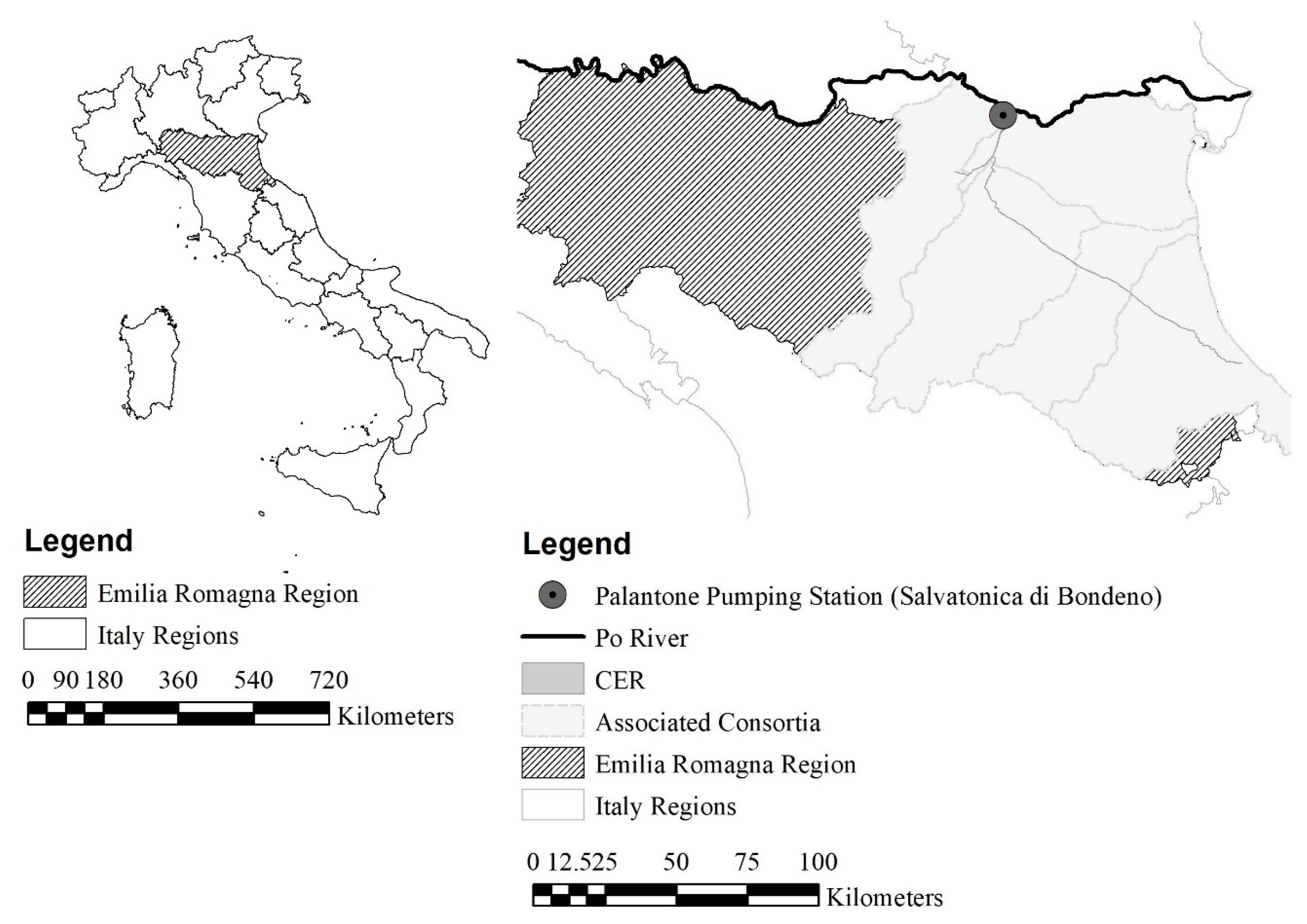
2.1. Description of the CER
2.2. Investigation Period and Available Data
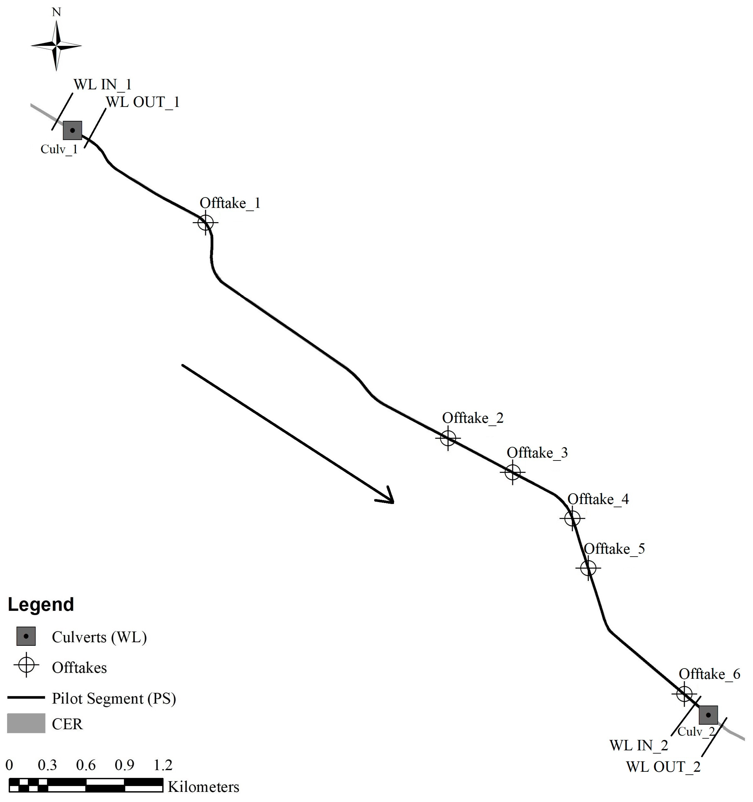
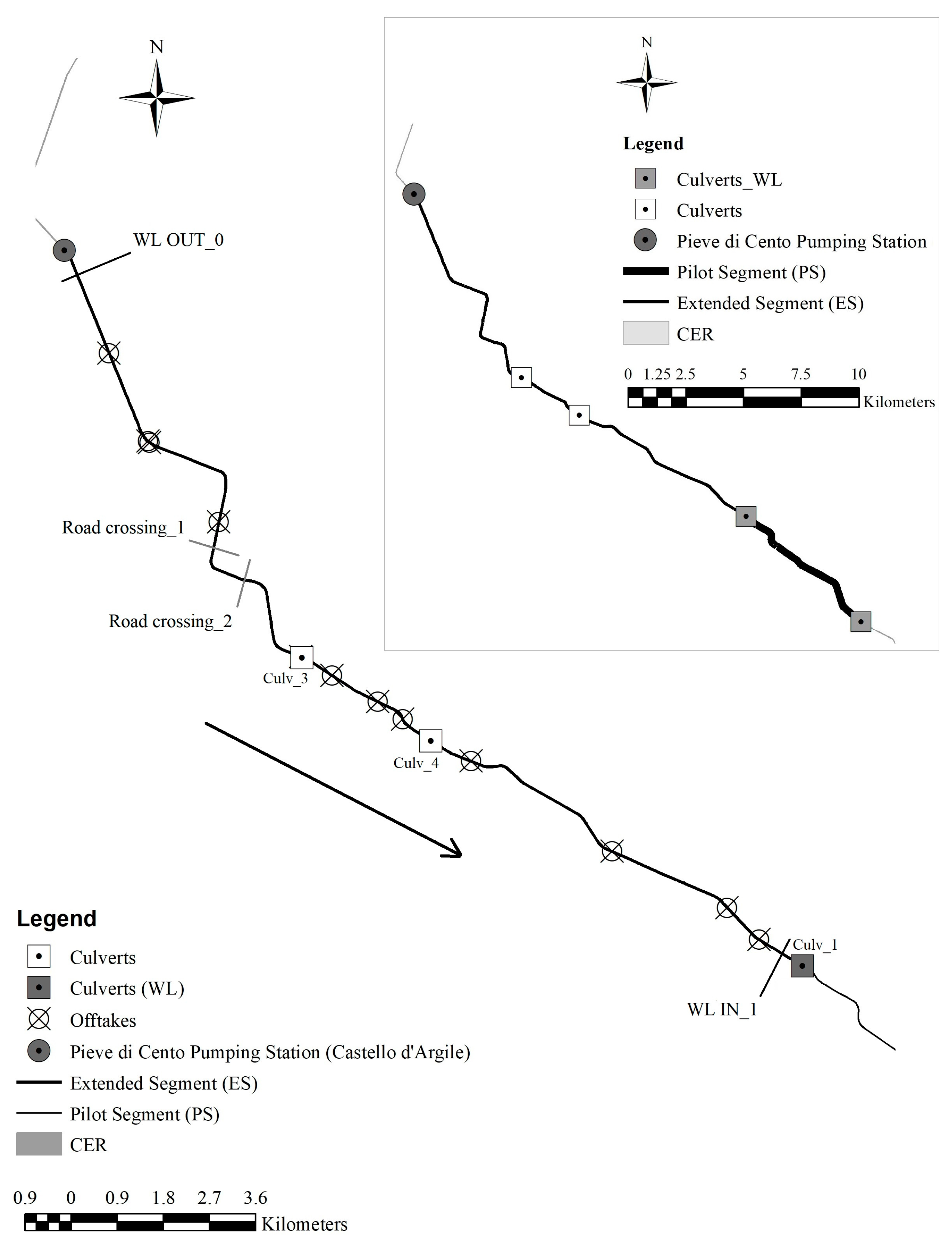
2.3. Description of the Pilot Segment (PS)
2.4. Elaboration of the Multi-Disciplinary Modelling Approach on PS
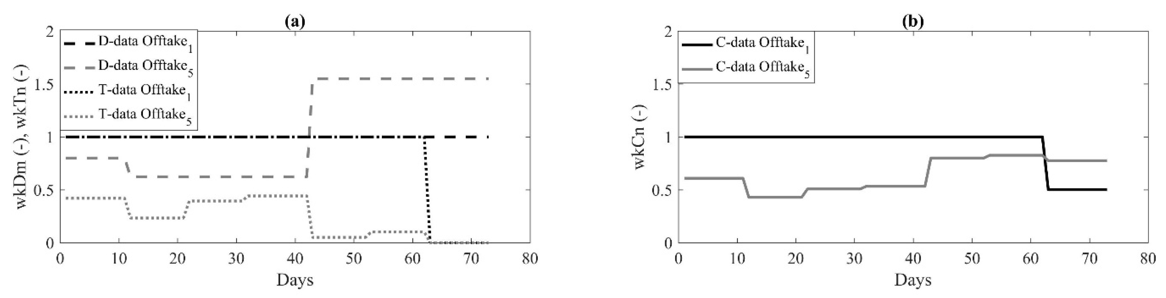
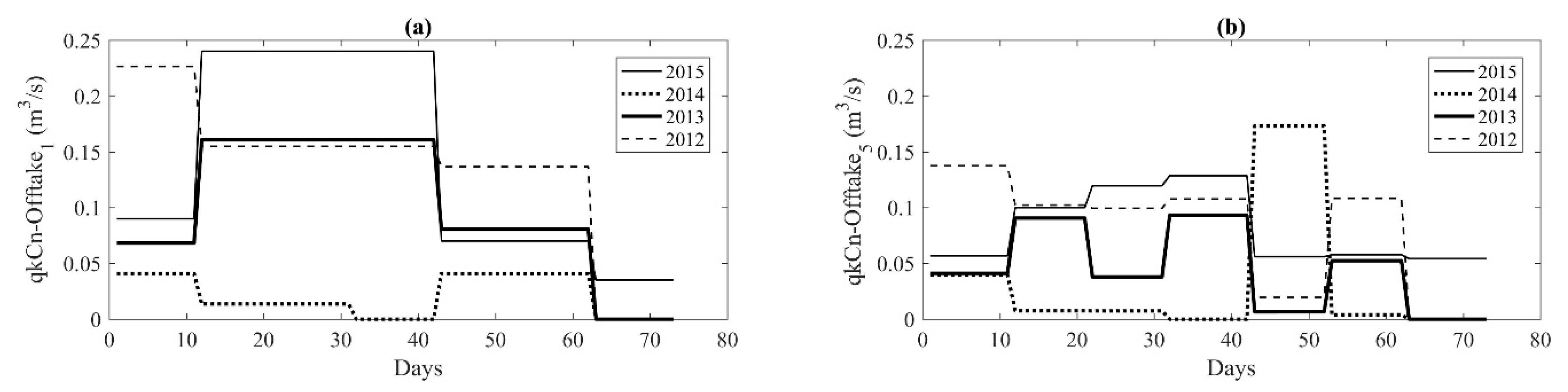
2.4.1. Reconstruction of the Unmeasured Offtake Discharges
2.4.2. Reconstruction of the Unmeasured Flowing Discharges
2.5. Description of the Extended Segment (ES)
2.6. Application of the Multi-disciplinary Modelling Approach on ES
3. Results and Discussion
3.1. Pilot Segment (PS)
3.1.1. Unmeasured Offtake Discharges
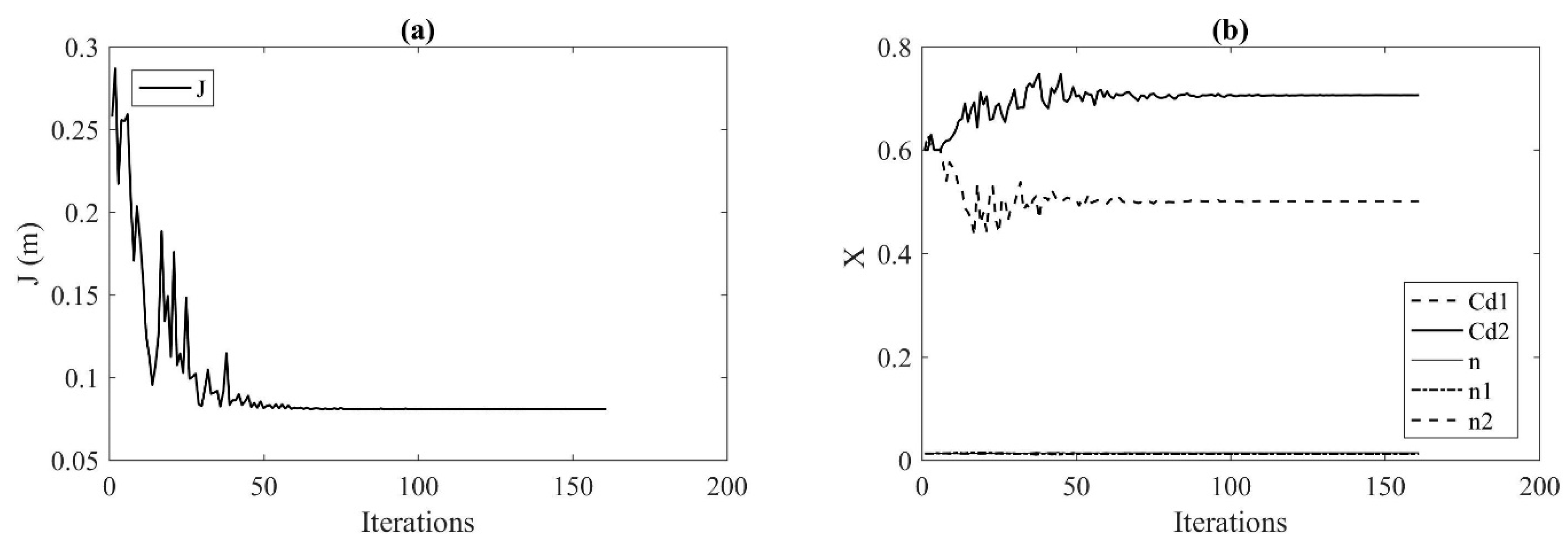
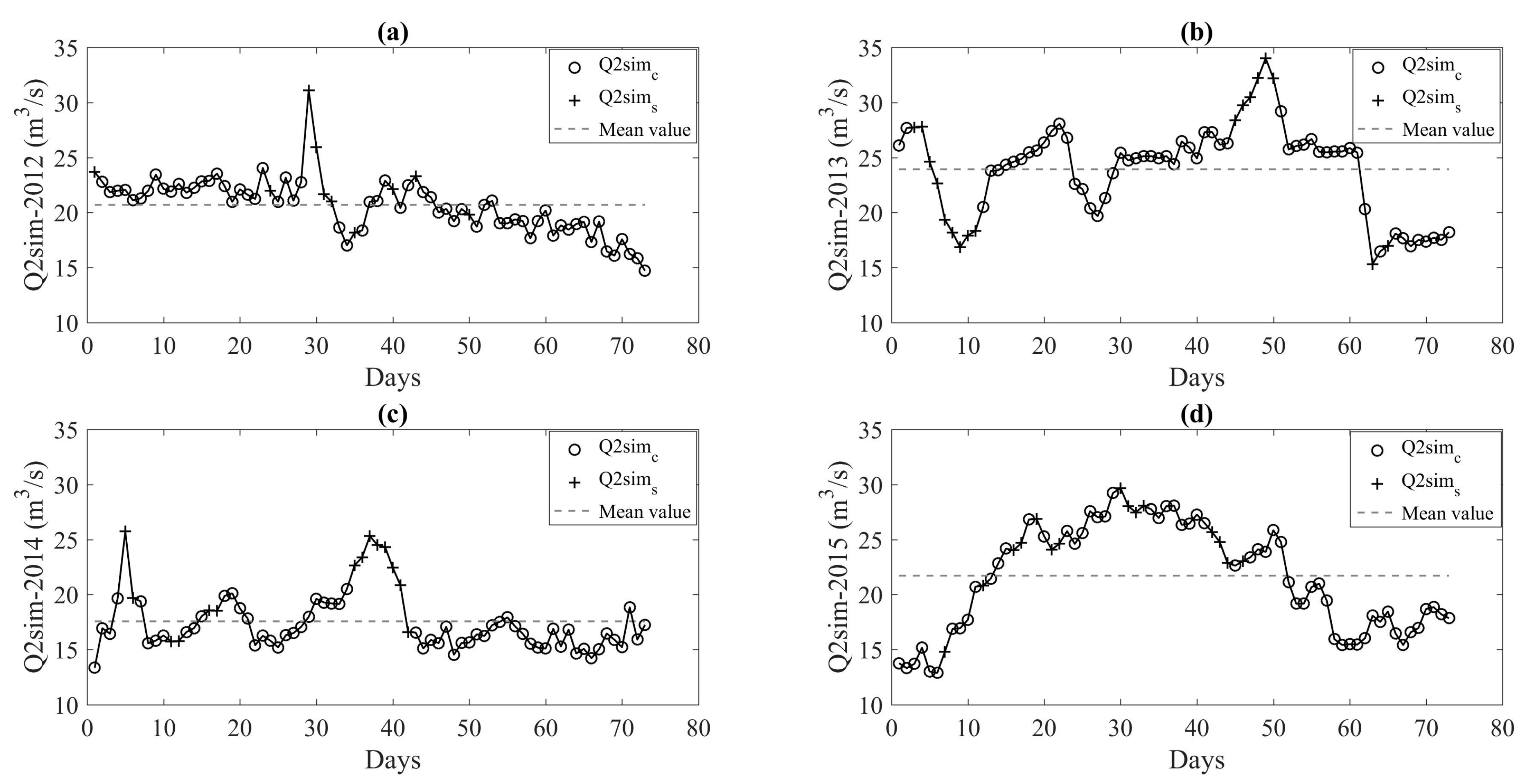
3.1.2. Steady State Flow Condition
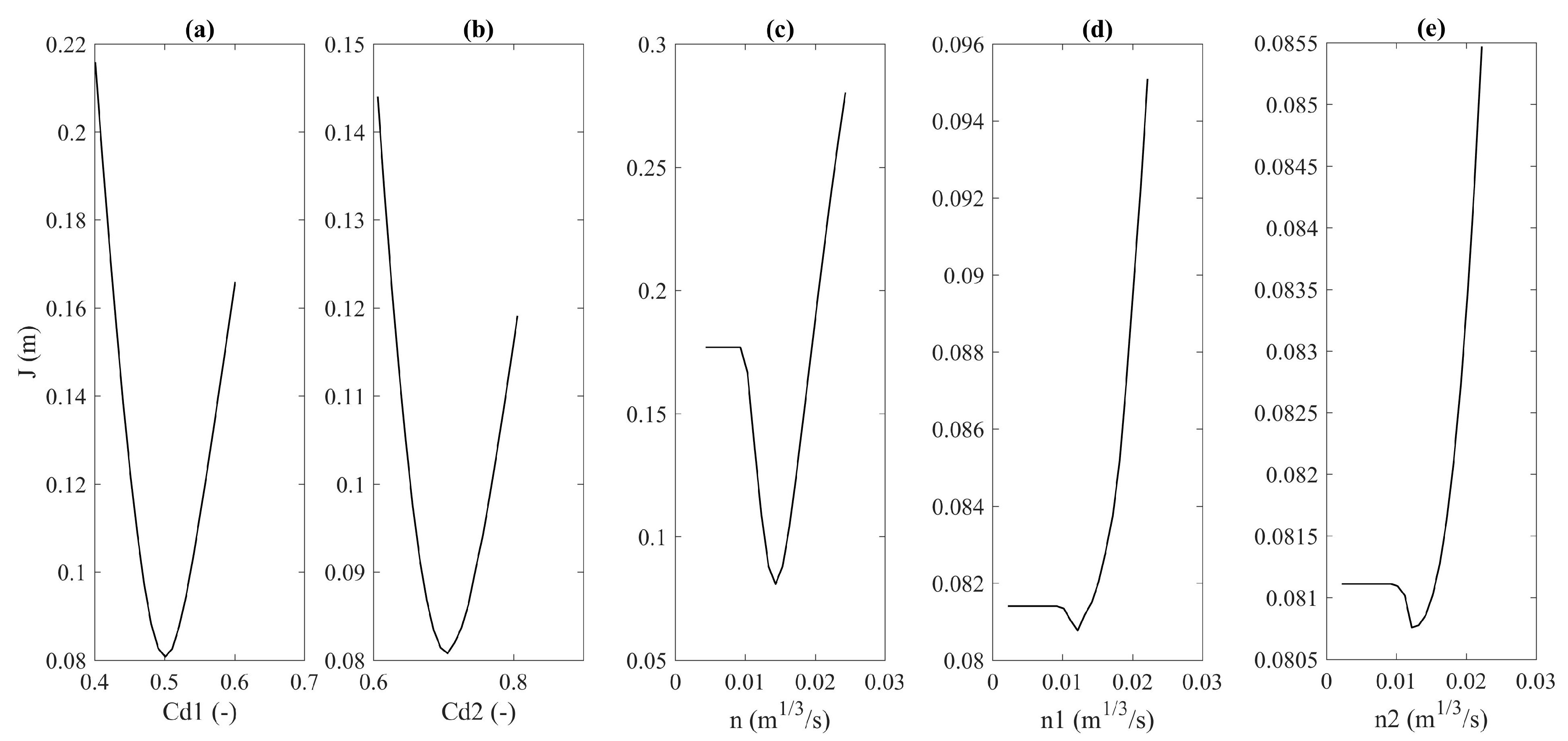
3.1.3. PS optimized Model
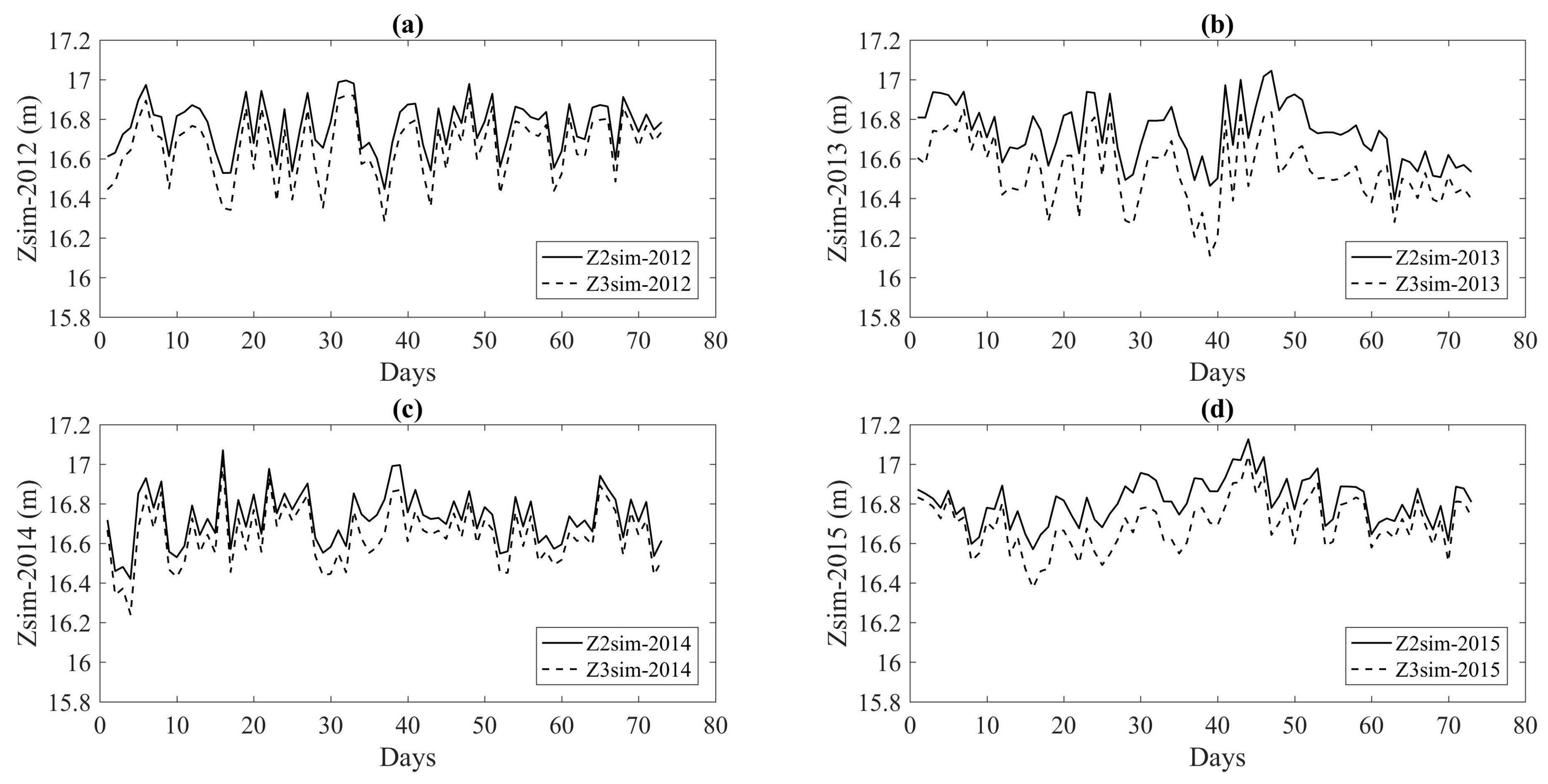
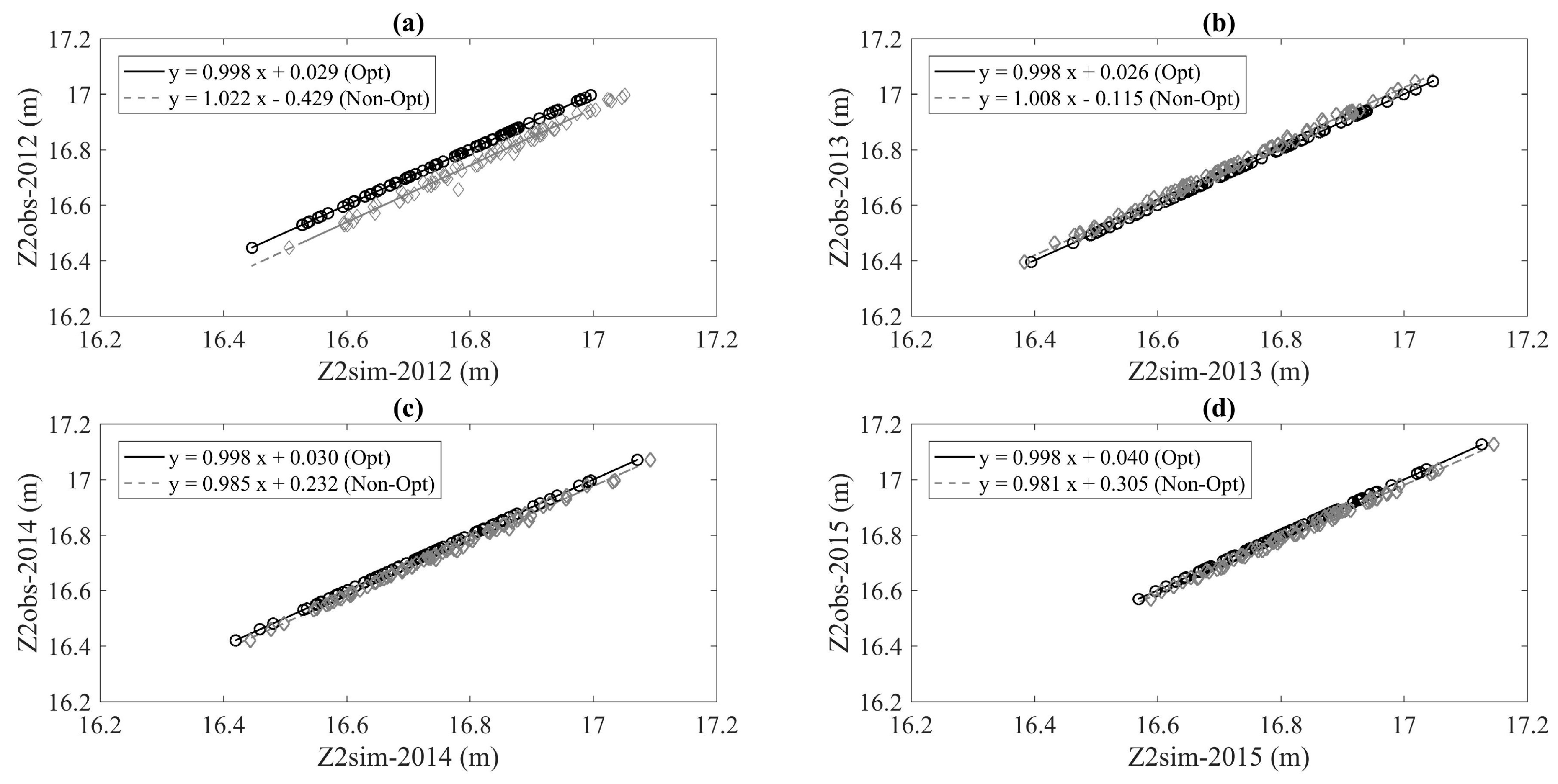
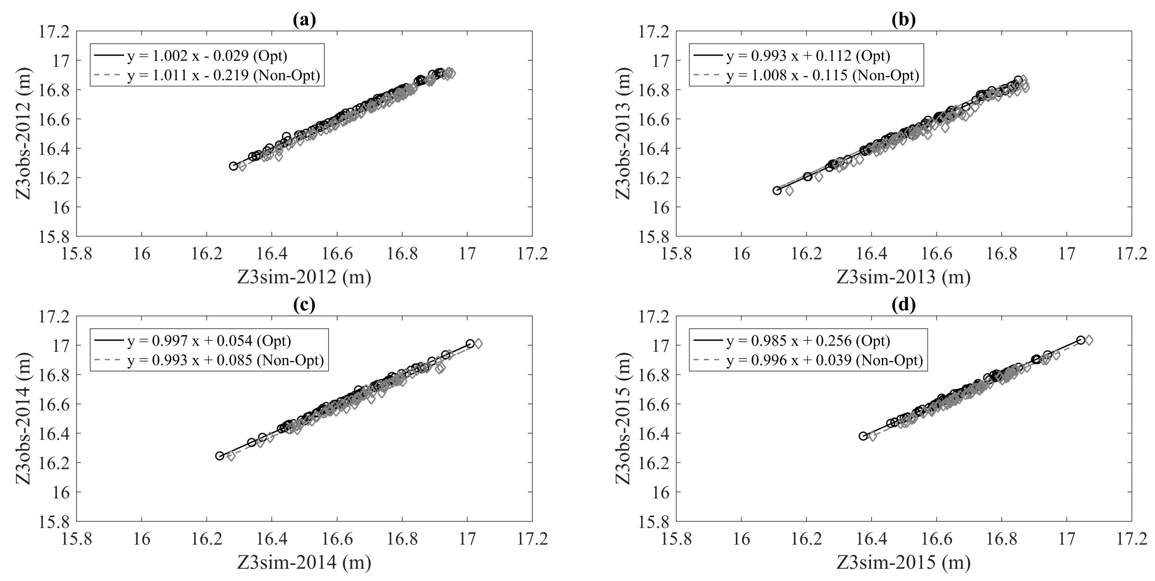
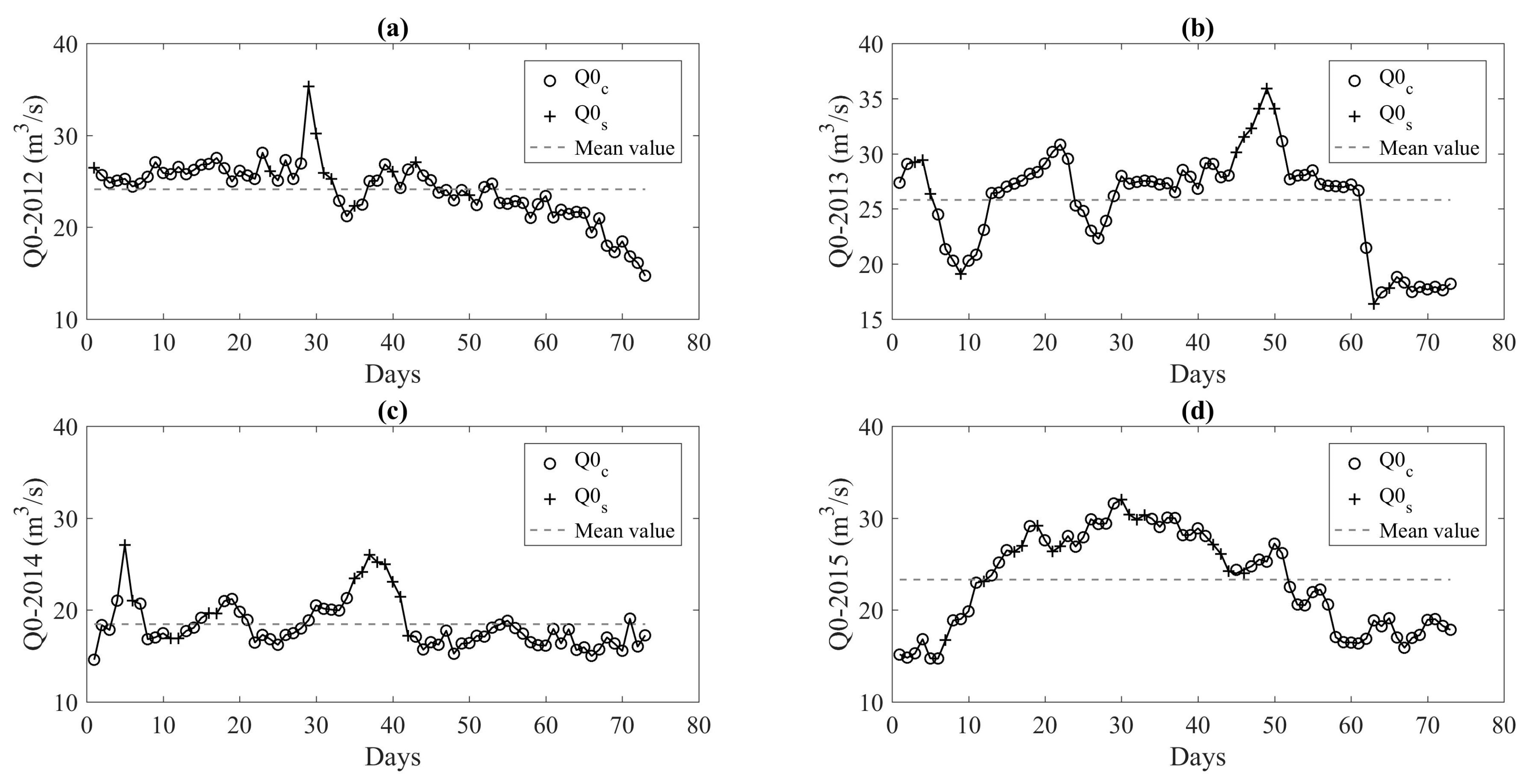
3.2. Extended Segment (ES)
4. Conclusions
Author Contributions
Funding
Acknowledgments
Conflicts of Interest
Abbreviations
| Along the CER | |
| Culv_1, Culv_2 | Culverts of Pilot Segment passing under rivers |
| Culv_3, Culv_4 | Culverts of Extended Segment passing under rivers |
| ES | Extended Segment |
| PS | Pilot Segment |
| WL OUT_0 | Water gauge at the exit of the pumping station Pieve di Cento |
| WL IN_1 | Water gauge at the entrance of Culv_1 |
| WL OUT_1 | Water gauge at the exit of Culv_1 |
| WL IN_2 | Water gauge at the entrance of Culv_2 |
| WL OUT_2 | Water gauge at the exit of Culv_2 |
| Measured data | |
| Z0obs,y | Vector containing daily water levels at WL OUT_0 for the year y |
| Z0pmax,y | Vector containing maximum daily water levels from the functioning of Pieve di Cento pumps |
| Z0pmin,y | Vector containing minimum daily water levels from the functioning of Pieve di Cento pumps |
| Z1obs,y | Vector containing daily water levels at WL IN_1 for the year y |
| Z2obs,y | Vector containing daily water levels at WL OUT_1 for the year y |
| Z3obs,y | Vector containing daily water levels at WL IN_2 for the year y |
| Z4obs,y | Vector containing daily water levels at WL OUT_2 for the year y |
| Offtakes | |
| Ai | Irrigable area; area covered by the crop i |
| C-data | Calculated data |
| CWRi | Decadal cumulated optimum crop water requirement for the crop i |
| D-data | Declared data provided by the Associated Consortia |
| Dm | Duration of the month m |
| ED | Coefficient of the efficiency of the delivery system CER-irrigable area |
| EIi | Coefficient of the efficiency of the irrigation method of the crop i |
| IIi | Coefficient of irrigation intensity of the crop i |
| qkCn | Calculated discharge exiting from the offtake k during the decade n |
| qkC,y | Vector containing daily calculated discharge values of the offtake k for the year y |
| qrDm | Discharge value exiting from the reference offtake during the month m |
| qtotC,y | Vector containing daily calculated offtake discharges from the segment (i.e., ES) for the year y |
| T-data | Estimated data provided by IRRINET |
| VkDm | Monthly cumulated volume of the offtake k from D-data |
| VkTn | Decadal cumulated volume of the offtake k from T-data |
| VrDm | Monthly cumulated volume of the reference offtake from the D-data |
| VrTn | Decadal cumulated volume of the reference offtake from the T-data |
| wkCn | Weight of the offtake k during the decade n |
| wkDm | Weight of the offtake k during the month m from D-data |
| wkTn | Weight of the offtake k during the decade n from T-data |
| Optimization | |
| Cd1, Cd2 | Gate discharge coefficients at the entrances of Culv_1 and Culv_2 |
| Cd3, Cd4 | Gate discharge coefficients at the entrances of Culv_3 and Culv_4 |
| Cd5, Cd6 | Gate discharge coefficients at the entrances of 2 road crossings (ES) |
| Cq | Scaling factor of the offtake discharges |
| J | Criteria to be minimized |
| n | Manning’s coefficient on the CER open-flow sections (along PS or ES) |
| n1, n2 | Manning’s coefficients within Culv_1 and Culv_2 |
| n3, n4 | Manning’s coefficients within Culv_3 and Culv_4 |
| n5, n6 | Manning’s coefficients within the 2 road crossings |
| Q0y | Vector containing daily calculated flowing discharges at WL OUT_0 for the year y |
| Q2sim,y | Vector containing daily simulated flowing discharges at WL OUT_1 for the year y |
| Q3sim,y | Vector containing daily simulated flowing discharges at WL IN_2 for the year y |
| Z0sim,y | Vector containing daily simulated water levels at WL OUT_0 for the year y |
| Z2sim,y | Vector containing daily simulated water levels at WL OUT_1 for the year y |
| Z3sim,y | Vector containing daily simulated water levels at WL IN_2 for the year y |
| σ0y | Vector containing the daily weights of the suspicious measures located in Z0obs,y |
| σ2y | Vector containing the daily weights of the suspicious measures located in Z1obs,y, Z2obs,y and Z4obs,y |
| σ3y | Vector containing the daily weights of the suspicious measures located in Z1obs,y, Z3obs,y and Z4obs,y |
References
- Sun, H.; Wang, S.; Hao, X. An Improved Analytic Hierarchy Process Method for the evaluation of agricultural water management in irrigation districts of north China. Agric. Water Manag. 2017, 179, 324–337. [Google Scholar] [CrossRef]
- Chen, S.; Ravallion, M. Absolute Poverty Measures for the Developing World, 1981–2004; PNAS: Washington, DC, USA, 2007. [Google Scholar]
- European Commission. Roadmap to a Resource Efficient Europe; European Environment Agency: Brussels, Belgium, 2011; pp. 1–24.
- Gordon, L.J.; Finlayson, C.M.; Falkenmark, M. Managing water in agriculture for food production and other ecosystem services. Agric. Water Manag. 2010, 97, 512–519. [Google Scholar] [CrossRef]
- De Fraiture, C.; Molden, D.; Wichelns, D. Investing in water for food, ecosystems, and livelihoods: An overview of the comprehensive assessment of water management in agriculture. Agric. Water Manag. 2010, 97, 495–501. [Google Scholar] [CrossRef]
- European Environmental Agency (EEA). Water Resources Across Europe-Confronting Water Scarcity and Drought; European Environment Agency: Copenhagen, Denmark, 2009; pp. 1–55.
- Molden, D. Water for Food, Water for Life: A Comprehensive Assessment of Water Management in Agriculture; Earthscan, IWMI: London, UK, 2007; pp. 1–39. [Google Scholar]
- Namara, R.E.; Hanjra, M.A.; Castillo, G.E.; Ravnborg, H.M.; Smith, L.; Koppen, B.V. Agricultural water management and poverty linkages. Agric. Water Manag. 2010, 97, 520–527. [Google Scholar] [CrossRef]
- Barker, R.; Molle, F. Evolution of irrigation in South and Southeast Asia, 2004. Available online: https://www.eea.europa.eu/publications/water-resources-across-europe (accessed on 27 July 2018).
- European Commission. Directive 2000/60/EC of the European Parliament and of the Council Establishing a Framework for the Community Action in the Field of Water Policy. Available online: https://www.eea.europa.eu/policy-documents/directive-2000-60-ec-of (accessed on 27 July 2018).
- European Commission DG ENV. Water Saving Potential in Agriculture in Europe: Findings from the Existing Studies and Applications; BIO Intelligence Service: Paris, France, 2012; pp. 1–232. [Google Scholar]
- Masseroni, D.; Ricart, S.; de Cartagena, F.; Monserrat, J.; Gonçalves, J.; de Lima, I.; Facchi, A.; Sali, G.; Gandolfi, C. Prospects for Improving Gravity-Fed Surface Irrigation Systems in Mediterranean European Contexts. Water 2017, 9, 20. [Google Scholar] [CrossRef]
- Levidow, L.; Zaccaria, D.; Maia, R.; Vivas, E.; Todorovic, M.; Scardigno, A. Improving water-efficient irrigation: Prospects and difficulties of innovative practices. Agric. Water Manag. 2014, 146, 84–94. [Google Scholar] [CrossRef]
- Ministero delle Politiche Agricole Alimentari e Forestali (MiPAAF). Approvazione delle linee guida per la regolamentazione da parte delle Regioni delle Modalità di quantificazione dei volumi idrici ad uso irriguo; MiPAAF: Rome, Italy, 2015. [Google Scholar]
- Litrico, X.; Fromion, V.; Baume, J.-P.; Arranja, C.; Rijo, M. Experimental validation of a methodology to control irrigation canals based on Saint-Venant Equations. Control Eng. Pract. 2005, 13, 1425–1437. [Google Scholar] [CrossRef]
- Lozano, D.; Arranja, C.; Rijo, M.; Mateos, L. Simulation of automatic control of an irrigation canal. Agric. Water Manag. 2010, 97, 91–100. [Google Scholar] [CrossRef]
- Cantoni, M.; Weyer, E.; Li, Y.; Ooi, S.K.; Mareels, I.; Ryan, M. Control of Large-Scale Irrigation Networks. Proc. IEEE 2007, 95, 75–91. [Google Scholar] [CrossRef]
- Ooi, S.K.; Weyer, E. Control design for an irrigation channel from physical data. Control Eng. Pract. 2008, 16, 1132–1150. [Google Scholar] [CrossRef]
- Jean-Baptiste, N.; Malaterre, P.-O.; Dorée, C.; Sau, J. Data assimilation for real-time estimation of hydraulic states and unmeasured perturbations in a 1D hydrodynamic model. Math. Comput. Simul. 2011, 81, 2201–2214. [Google Scholar] [CrossRef]
- Jeroen, V.; Linden, V. Volumetric water control in a large-scale open canal irrigation system with many smallholders: The case of chancay-lambayeque in Peru. Agric. Water Manag. 2011, 98, 705–714. [Google Scholar]
- Islam, A.; Raghuwanshi, N.S.; Singh, R. Development and application of hydraulic simulation model for irrigation canal network. J. Irrig. Drain. Eng. 2008, 134, 49–59. [Google Scholar] [CrossRef]
- Renault, D. Aggregated hydraulic sensitivity indicators for irrigation system behavior. Agric. Water Manag. 2000, 43, 151–171. [Google Scholar] [CrossRef]
- Cornish, G.; Bosworth, B.; Perry, C.; Burke, J. Water Charging in Irrigated Agriculture: An Analysis of International Experience. Available online: http://www.fao.org/docrep/008/y5690e/y5690e00.htm (accessed on 6 June 2018).
- Laycock, A. Irrigation Systems: Design, Planning and Construction; CAB International: Wallingford, UK, 2007; pp. 1–285. [Google Scholar]
- Molle, F. Water scarcity, prices and quotas: A review of evidence on irrigation volumetric pricing. Irrig. Drain. Syst. 2009, 23, 43–58. [Google Scholar] [CrossRef]
- Food and Agriculture Organization of the United Nations (FAO). The State of the World’s Land and Water Resources for Food and Agriculture (SOLAW)—Managing Systems at Risk; Food and Agriculture Organization of the United Nations: Rome, Italy, 2011; pp. 1–281. [Google Scholar]
- Rault, P.K.; Jeffrey, P. On the appropriateness of public participation in integrated water resources management: Some grounded insights from the Levant. Integr. Assess. 2008, 8, 69–106. [Google Scholar]
- Huang, Y.; Fipps, G. Developing a modeling tool for flow profiling in irrigation distribution networks. Int. J. Agric. Biol. Eng. 2009, 2, 17–26. [Google Scholar]
- Tariq, J.A.; Latif, M. Improving operational performances of farmers managed distributary canal using SIC hydraulic model. Water Resour. Manag. 2010, 24, 3085–3099. [Google Scholar] [CrossRef]
- Sau, J.; Malaterre, P.O.; Baume, J.P. Sequential Monte Carlo hydraulic state estimation of an irrigation canal. Comptes Rendus Mécanique 2010, 338, 212–219. [Google Scholar] [CrossRef]
- Kumar, P.; Mishra, A.; Raghuwanshi, N.S.; Singh, R. Application of unsteady flow hydraulic-model to a large and complex irrigation system. Agric. Water Manag. 2002, 54, 49–66. [Google Scholar] [CrossRef]
- Giupponi, C. Decision Support Systems for implementing the European Water Framework Directive: The MULINO approach. Environ. Model. Softw. 2007, 22, 248–258. [Google Scholar] [CrossRef]
- Mateos, L.; Lopez-Cortijo, I.; Sagardoy, J. SIMIS the FAO decision support system for irrigation scheme management. Agric. Water Manag. 2002, 56, 193–206. [Google Scholar] [CrossRef]
- Leenhardt, D.; Trouvat, J.L.; Gonzalès, G.; Pérarnaud, V.; Prats, S.; Bergez, J.E. Estimating irrigation demand for water management on a regional scale. Agric. Water Manag. 2004, 68, 207–232. [Google Scholar] [CrossRef]
- Mailhol, J.-C. Evaluation à l’échelle Régionale des Besoins en Eau et du Rendement des Cultures Selon la Disponibilité en eau. Application au bassin Adour-Garonne; Agence de l’Eau Adour-Garonne: Toulouse, France, 1992; pp. 1–24. [Google Scholar]
- Sousa, V.; Santos Pereira, L. Regional analysis of irrigation water requirements using kriging. Application to potato crop (Solanum tuberosum L.) at Tras-os-Montes. Agric. Water Manag. 1999, 40, 221–233. [Google Scholar] [CrossRef]
- Heinemann, A.B.; Hoogenboom, G.; Faria de, R.T. Determination of spatial water requirements at county and regional levels using crop models and GIS: An example for the state of Parana, Brazil. Agric. Water Manag. 2002, 52, 177–196. [Google Scholar] [CrossRef]
- Kinzli, K.-D.; Gensler, D.; Oad, R.; Shafike, N. Implementation of a decision support system for improving irrigation water delivery: Case study. Irrig. Drain. Syst. 2015, 141, 05015004. [Google Scholar] [CrossRef]
- Miao, Q.; Shi, H.; Gonçalves, J.; Pereira, L. Basin irrigation design with multi-criteria analysis focusing on water saving and economic returns: Application to wheat in Hetao, Yellow River Basin. Water 2018, 10, 67. [Google Scholar] [CrossRef]
- Yang, G.; Liu, L.; Guo, P.; Li, M. A flexible decision support system for irrigation scheduling in an irrigation district in China. Agric. Water Manag. 2017, 179, 378–389. [Google Scholar] [CrossRef]
- Tanure, S.; Nabinger, C.; Becker, J.L. Bioeconomic model of decision support system for farm management: Proposal of a mathematical model: Bioeconomic model of decision support system for farm management. Syst. Res. Behav. Sci. 2015, 32, 658–671. [Google Scholar] [CrossRef]
- Consortium of the Canale Emiliano Romagnolo (CER). Available online: http://www.consorziocer/ (accessed on 17 May 2018).
- Istituto Nazionale di Statistica (ISTAT). Censimento Agricoltura 2010. Available online: http://www4.istat.it/it/censimento-agricoltura/agricoltura-2010 (accessed on 22 May 2018).
- Munaretto, S.; Battilani, A. Irrigation water governance in practice: The case of the Canale Emiliano Romagnolo district, Italy. Water Policy 2014, 16, 578. [Google Scholar] [CrossRef]
- Service IRRIFRAME. Available online: https://ssl.altavia.eu/Irriframe/ (accessed on 29 October 2017).
- Delibera di Giunta Regionale (DGR). Bollettino Ufficiale della Regione Emilia Romagna, Parte Seconda, n.9—Deliberazione della Giunta Regionale 21 Dicembre 2016, n. 2254; Giunta Regionale: Bologne, Italy, 2016; pp. 1–10. (In Italian) [Google Scholar]
- Mannini, P.; Genovesi, R.; Letterio, T. IRRINET: Large scale DSS application for on-farm irrigation scheduling. Procedia Environ. Sci. 2013, 19, 823–829. [Google Scholar] [CrossRef]
- Singley, B.C.; Hotchkiss, R.H. Differences between Open-Channel and Culvert Hydraulics: Implications for Design. 2010. Available online: https://doi.org/10.1061/41114 (accessed on 27 July 2018).
- Software SIC2. Available online: http://sic.g-eau.net/ (accessed on 30 October 2017).
- Haque, S. Impact of irrigation on cropping intensity and potentiality of groundwater in murshidabad district of West Bengal, India. Int. J. Ecosyst. 2015, 5, 55–64. [Google Scholar]
- Thenkabail, P.; Dheeravath, V.; Biradar, C.; Gangalakunta, O.R.; Noojipady, P.; Gurappa, C.; Velpuri, M.; Gumma, M.; Li, Y. Irrigated area maps and statistics of India using remote sensing and national statistics. Remote Sens. 2009, 1, 50–67. [Google Scholar] [CrossRef]
- Tanriverdi, C.; Degirmenci, H.; Sesveren, S. Assessment of irrigation schemes in Turkey: Cropping intensity, irrigation intensity and water use. In Proceedings of the Tropentag 2015, Berlin, Germany, 16–18 September 2015. [Google Scholar]
- Battilani, A. L’irrigazione del medicaio. Agricoltura 1994, 3, 31–33. [Google Scholar]
- Battilani, A. Regulated deficit of irrigation (RDI) effects on growth and yield of plum tree. Acta Hortic. 2004, 664, 55–62. [Google Scholar] [CrossRef]
- Battilani, A.; Anconelli, S.; Guidoboni, G. Water table level effect on the water balance and yield of two pear rootstock. Acta Hortic. 2004, 664, 47–54. [Google Scholar] [CrossRef]
- Battilani, A.; Ventura, F. Influence of water table, irrigation and rootstock on transpiration rate and fruit growth of peach trees. Acta Hortic. 1996, 449, 521–528. [Google Scholar] [CrossRef]
- Food and Agriculture Organization of the United Nations (FAO). Irrigation Water Management: Irrigation Scheduling, Training Manual n.4. 1989. Available online: http://www.fao.org/docrep/t7202e/t7202e08.htm (accessed on 21 June 2017).
- Delibera di Giunta Regionale (DGR). Bollettino Ufficiale della Regione Emilia Romagna, Parte Seconda, n.327—Deliberazione della Giunta Regionale 5 Settembre 2016, n. 1415; Giunta Regionale: Bologne, Italy, 2016; pp. 1–11. (In Italian) [Google Scholar]
- Artina, S.; Montanari, A. Consulenza per lo Studio delle Perdite Idriche nelle Reti di Distribuzione dei Consorzi di Bonifica; Università degli Studi di Bologna: Bologne, Italy, 2007; pp. 1–46. (In Italian) [Google Scholar]
- Taglioli, G.; Cinti, P. Water Losses of Land Channels [Emilia-Romagna]. Rivista di Ingegneria Agraria. 2002. Available online: http://agris.fao.org/agris-search/search.do?recordID=IT2004060023 (accessed on 27 July 2018).
- Consorzio della Bonifica Renana. Available online: https://www.bonificarenana.it/ (accessed on 11 July 2018).
- Gejadze, I.; Malaterre, P.O. Discharge estimation under uncertainty using variational methods with application to the full Saint-Venant hydraulic network model: Discharge estimation under uncertainty using variational methods. Int. J. Numer. Methods Fluids 2017, 83, 405–430. [Google Scholar] [CrossRef]
- Oubanas, H.; Gejadze, I.; Malaterre, P.O. River discharge estimation under uncertainty from synthetic SWOT-type observations using variational data assimilation. Contribution of the UMR G−eau investigation team, IRSTEA Montpellier, France to the SWOT mission. La Houille Blanche 2018, 2, 84–89. [Google Scholar] [CrossRef]
- Baume, J.P.; Malaterre, P.O.; Benoit, G.B. SIC: A 1D Hydrodynamic Model for River and Irrigation Canal Modeling and Regulation; CEMAGREF, Agricultural and Environmental Engineering Research: Montpellier, France, 2005; pp. 1–81. [Google Scholar]
- Sau, J.; Malaterre, P.-O.; Baume, J.P. Sequential Monte Carlo hydraulic state estimation of an irrigation canal. Comptes Rendus Mécanique 2010, 338, 212–219. [Google Scholar] [CrossRef]
- Cunge, J.; Holly, F.M.; Verwey, A., Jr. Practical Aspects of Computational Rive Hydraulics; Pitman Advanced Pub. Program: Boston, MA, USA, 1980; pp. 1–420. [Google Scholar]
- Chaudhry, H.M. Open Channel Flow, 2nd ed.; Springer: New York, NY, USA, 2007; pp. 1–517. [Google Scholar]
- Baume, J.-P.; Belaud, G.; Vion, P.Y. Hydraulique Pour le Génie Rural Notes de Cours; Ecole Nationale Supérieure d’Agronomie, CEMAGREF: Montpellier, France, 2006; pp. 1–179. [Google Scholar]
- Nielsen, K.D.; Weber, L.J. Submergence effects on discharge coefficients for rectangular. In Proceedings of the Joint Conference on Water Resource Engineering and Water Resources Planning and Management 2000, Minneapolis, MN, USA, 30 July–2 August 2000. [Google Scholar]
- Nelder, J.A.; Mead, R. A simplex method for function minimization. Comput. J. 1965, 7, 308–313. [Google Scholar] [CrossRef]
- United States Bureau of Reclamation (USBR). Water Measurement Manual; Water Resources: Englewood, CO, USA, 1997.
- Wu, S.; Rajaratnam, N. Solutions to rectangular sluice gate flow problems. J. Irrig. Drain. Eng. 2015, 141, 06015003. [Google Scholar] [CrossRef]
- Sauida, M.F. Calibration of submerged multi-sluice gates. Alexandria Eng. J. 2014, 53, 663–668. [Google Scholar] [CrossRef]
- Chow, V.T. Open-Channel Hydraulics; McGraw-Hill: New York, NY, USA, 1959; pp. 1–680. [Google Scholar]
- De Doncker, L.; Troch, P.; Verhoeven, R.; Bal, K.; Meire, P.; Quintelier, J. Determination of the manning roughness coefficient influenced by vegetation in the river Aa and Biebrza river. Environ Fluid Mech. 2009, 9, 549–567. [Google Scholar] [CrossRef]
- Dyhouse, G.; Hatchett, J.; Benn, J. Floodplain Modeling Using HEC-RAS; Haestad Press: Aterbury, CT, USA, 2003; pp. 1–1261. [Google Scholar]
- Tedeschi, L.O. Assessment of the adequacy of mathematical models. Agric. Syst. 2006, 89, 225–247. [Google Scholar] [CrossRef]
- St-Pierre, N.R. Comparison of model predictions with measurements: A novel model-assessment method. J. Dairy Sci. 2016, 99, 4907–4927. [Google Scholar] [CrossRef] [PubMed]
- Harrison, S.R. Validation of agricultural expert systems. Agric. Syst. 1991, 35, 265–285. [Google Scholar] [CrossRef]
- Mayer, D.G.; Butler, D.G. Statistical validation. Ecol. Model. 1993, 68, 21–32. [Google Scholar] [CrossRef]
- Mayer, D.G.; Stuart, M.A.; Swain, A.J. Regression of real-world data on model output: An appropriate overall test of validity. Agric. Syst. 1994, 45, 93–104. [Google Scholar] [CrossRef]
- Dent, J.B.; Blackie, M.J. Systems Simulation in Agriculture; Applied Science: London, UK, 1979. [Google Scholar]
- Mesplé, F.; Troussellier, M.; Casellas, C.; Legendre, P. Evaluation of simple statistical criteria to qualify a simulation. Ecol. Model. 1996, 88, 9–18. [Google Scholar] [CrossRef]


| Available Data | Type | Unit | Time Step | Source |
|---|---|---|---|---|
| Offtake Volumes | Indirectly calculated | m3 | Monthly (cumulated values) | Associated Consortia |
| CWRi | Estimated | mm | Decadal (cumulated values) | IRRINET |
| Water Levels | Measured | m | Daily (average values) | CER |
| Water Levels at Suction/Delivery Tanks | Measured | m | Pumps on/off (single values) | CER |
| Irrigated Crops | IIi (-) | EIi (-) |
|---|---|---|
| Extensive crops | ||
| Maize | 0.75 | 0.75 |
| Soy | 0.50 | 0.75 |
| Alfa-Alfa | 0.25 | 0.75 |
| Vegetables | ||
| Beet | 0.60 | 0.75 |
| Onion | 1.00 | 0.75 |
| Melon | 1.00 | 0.85 |
| Potato | 1.00 | 0.75 |
| Tomato | 1.00 | 0.85 |
| Orchards | ||
| Pear | 1.00 | 0.85 |
| Peach | 1.00 | 0.85 |
| Vine | 0.50 | 0.85 |
| Year | Parameterized Hydraulic Variables | Cost of the Criterion | ||||
|---|---|---|---|---|---|---|
| Cd1 (-) | Cd2 (-) | n (m1/3/s) | n1 (m1/3/s) | n2 (m1/3/s) | J Cost (m) | |
| Without Suspicious Measures Weights | ||||||
| 2012 | 0.37 | 0.64 | 0.014 | 0.015 | 0.015 | 0.1742 |
| 2013 | 0.68 | 0.76 | 0.015 | 0.009 | 0.011 | 0.2799 |
| 2014 | 0.39 | 0.82 | 0.016 | 0.015 | 0.008 | 0.2331 |
| 2015 | 0.49 | 0.69 | 0.015 | 0.012 | 0.013 | 0.1036 |
| With Suspicious Measures Weights | ||||||
| 2012 | 0.37 | 0.65 | 0.014 | 0.014 | 0.015 | 0.1460 |
| 2013 | 0.71 | 0.74 | 0.016 | 0.009 | 0.011 | 0.1480 |
| 2014 | 0.44 | 0.80 | 0.015 | 0.013 | 0.010 | 0.1101 |
| 2015 | 0.50 | 0.71 | 0.014 | 0.012 | 0.012 | 0.0808 |
| Year | RMSE (m) | |
|---|---|---|
| Non-Optimized Hydraulic Model | Optimized Hydraulic Model | |
| WL OUT_1 | ||
| 2012 | 0.0586 | 2.9 × 10⁻⁴ |
| 2013 | 0.0220 | 6.1 × 10⁻⁴ |
| 2014 | 0.0216 | 5.8 × 10⁻⁴ |
| 2015 | 0.0185 | 3.9 × 10⁻⁴ |
| WL IN_2 | ||
| 2012 | 0.0318 | 6.1 × 10⁻³ |
| 2013 | 0.0340 | 11.2 × 10⁻³ |
| 2014 | 0.0316 | 8.3 × 10⁻³ |
| 2015 | 0.0265 | 7.0 × 10⁻³ |
| Year | Parameterized Hydraulic Variables | Cost of the Criterion | ||||||||
|---|---|---|---|---|---|---|---|---|---|---|
| Cd3 (-) | Cd4 (-) | Cd5 (-) | Cd6 (-) | n (m1/3/s) | n3 (m1/3/s) | n4 (m1/3/s) | n5 (m1/3/s) | n6 (m1/3/s) | J Cost (m) | |
| 2012 | 0.60 | 0.45 | 0.62 | 0.52 | 0.020 | 0.020 | 0.013 | 0.011 | 0.010 | 0.5057 |
| 2013 | 0.58 | 0.60 | 0.58 | 0.58 | 0.014 | 0.013 | 0.013 | 0.013 | 0.013 | 0.4667 |
| 2015 | 0.42 | 0.59 | 0.43 | 0.45 | 0.011 | 0.019 | 0.019 | 0.019 | 0.010 | 0.3465 |
© 2018 by the authors. Licensee MDPI, Basel, Switzerland. This article is an open access article distributed under the terms and conditions of the Creative Commons Attribution (CC BY) license (http://creativecommons.org/licenses/by/4.0/).
Share and Cite
Luppi, M.; Malaterre, P.-O.; Battilani, A.; Di Federico, V.; Toscano, A. A Multi-disciplinary Modelling Approach for Discharge Reconstruction in Irrigation Canals: The Canale Emiliano Romagnolo (Northern Italy) Case Study. Water 2018, 10, 1017. https://doi.org/10.3390/w10081017
Luppi M, Malaterre P-O, Battilani A, Di Federico V, Toscano A. A Multi-disciplinary Modelling Approach for Discharge Reconstruction in Irrigation Canals: The Canale Emiliano Romagnolo (Northern Italy) Case Study. Water. 2018; 10(8):1017. https://doi.org/10.3390/w10081017
Chicago/Turabian StyleLuppi, Marta, Pierre-Olivier Malaterre, Adriano Battilani, Vittorio Di Federico, and Attilio Toscano. 2018. "A Multi-disciplinary Modelling Approach for Discharge Reconstruction in Irrigation Canals: The Canale Emiliano Romagnolo (Northern Italy) Case Study" Water 10, no. 8: 1017. https://doi.org/10.3390/w10081017
APA StyleLuppi, M., Malaterre, P.-O., Battilani, A., Di Federico, V., & Toscano, A. (2018). A Multi-disciplinary Modelling Approach for Discharge Reconstruction in Irrigation Canals: The Canale Emiliano Romagnolo (Northern Italy) Case Study. Water, 10(8), 1017. https://doi.org/10.3390/w10081017