Article

Intercomparison of a Lumped Model and a Distributed Model for Streamflow Simulation in the Naoli River Watershed, Northeast China

1
Key Laboratory of Poyang Lake Wetland and Watershed Research, Ministry of Education, School of Geography and Environment, Jiangxi Normal University, Nanchang 330022, China
2
Jiangxi Weather Modification Office, Nanchang 30096, China
3
College of Biology and the Environment, Nanjing Forestry University, Nanjing 210037, China
*
Author to whom correspondence should be addressed.
Water 2018, 10(8), 1004; https://doi.org/10.3390/w10081004
Submission received: 9 May 2018 / Revised: 5 July 2018 / Accepted: 19 July 2018 / Published: 30 July 2018
(This article belongs to the Special Issue Catchment Modelling)

Abstract

:
Water supply availability has significant impacts on the biggest base for commodity grain production: The Sanjiang Plain in northeast China. The SWAT (soil and water assessment tool) model and IHACRES (identification of unit hydrographs and component flows from rainfall, evapotranspiration and streamflow data) model were used for modelling streamflow variability in the upper Naoli River watershed to determine the applicability of hydrological models to the marsh rivers. Both the SWAT and IHACRES models were suitable for streamflow simulation, having R2 (coefficient of determination) and NS (Nash–Sutcliffe) values greater than 0.7, and PBIAS (percent bias) smaller than 25%. The IHACRES model was easy to use, with less data-preparation, and was found to be a better choice for runoff simulation in a watershed less affected by human activity. The simulation result was better in primeval times, i.e., 1956–1966, than the period 1967–2005, when its performance was found to be unfavorable. In contrast, the complex, processes-based SWAT model was found to be more appropriate for simultaneously simulating streamflow variability. In addition, the effects of land use change and human activities in the watershed—where agricultural activities are intensive—were evaluated. The study found that the SWAT model was potentially suitable for water resource planning and management.

1. Introduction

Wetlands, which cover 5–8% of the land surface of the Earth, play an important role in flood control, regulating runoff, water quality improvement, biodiversity protection, and so on [1]. The Sanjiang plain, located in northeast China, is the largest distribution area of marsh in China. It was reclaimed for agricultural production and has since become the biggest base for commodity grain production in China [2,3,4]. Located in the center of the Sanjiang Plain, the Naoli River watershed is a marsh river and a typical aquatic community. The hydrological processes associated with the watershed have an extremely important role in wetland formation, wetland development, wetland evolution and wetland disappearance [5]. Hydrological element variations are influenced by drastic changes, deriving from anthropogenic effects or natural disasters [6,7]. This area was mostly covered by natural freshwater wetlands in the early 1950s, and has since experienced intensive reclamation [8,9]. The effects of climate change and land use are expected to further complicate the already fragile hydrological cycle system in the Naoli River watershed [10,11]. Thus, the research of streamflow variation has become a critical issue in this area.
The research methods that have been employed include time series analysis, paired catchment studies and hydrological modeling [12,13]. Paired catchment studies are difficult to extend to large catchments, while the method of time series analysis is limited because of a lack of a physical mechanism. The impacts of climate change and agricultural development on water resources are difficult to quantify by statistical analyses. Therefore, hydrological models are often used to provide some important information for water resource management decisions. Hydrological models are considered to be preferable methods for researching streamflow variability [14,15,16]. Different models are selected based on specific research purposes. Two types of hydrological models, namely the physically-based models and the conceptual models, are often used to predict watershed streamflow responses. The physically-based models (e.g., the soil and water assessment tool or SWAT model) have been widely used in the hydrological literature, which attempt to take full account of the spatial variability, such as land use change and climate variability [17,18]. However, sometimes these have no advantage over conceptual models (e.g., the identification of unit hydrographs and component flows from rainfall, evapotranspiration and streamflow data or IHACRES model), either in terms of data preparation or in their predictive ability [19,20,21]. Moreover, there are ungauged basins of the Sanjiang Plain which lack land use and hydro-meteorological data due to harsh observed conditions or high monitoring cost. Therefore, in this study, both a physically-based model and a conceptual model were chosen for variation process analysis of the hydrologic elements.
Currently, the majority of research in this area is based on statistical analyses without adequate quantitative analysis of hydrologic change. In addition, there is a dearth of research on the application of a model simulation in the Naoli River watershed. In this study, the SWAT model was used for runoff simulation and was compared with the IHACRES model. The major purposes of the study were to (1) evaluate the SWAT model performance and assess the feasibility of using SWAT for hydrologic modeling in the upper Naoli River watershed, and (2) compare simulation results between the SWAT and IHACRES model to provide advice on model selection for streamflow variation in the Naoli River watershed.

2. Materials and Methods

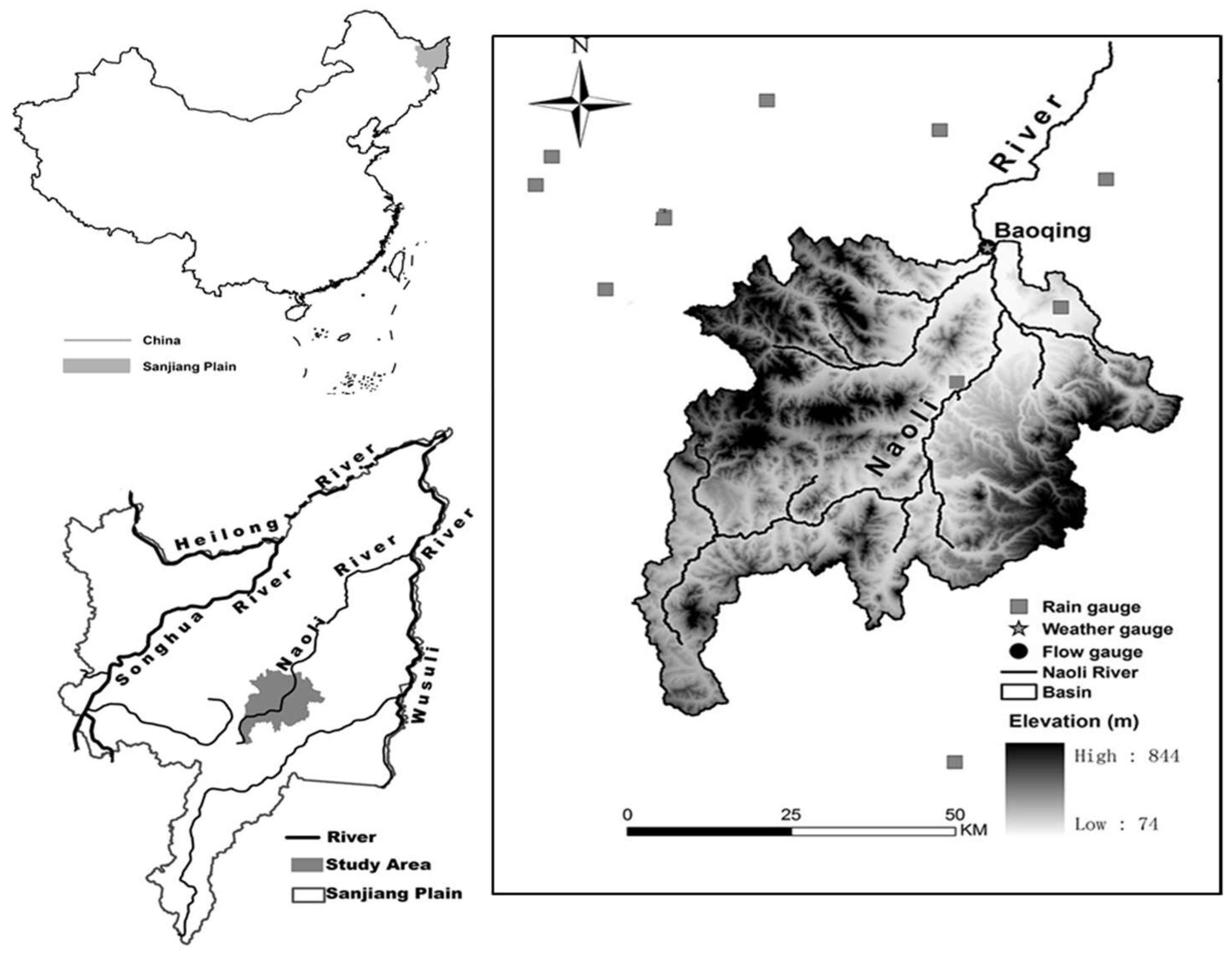
2.1. Study Site and Data Collection

The Naoli River watershed lies between latitude 45°43′ and 47°45′ N and longitude 131°31′ to 134°10′ E. The total basin area is about 24,863 km2, accounting for about 25% of the total area of the Sanjiang Plain, of which 33.5% is mountainous area, 61.7% is plains, and 4.8% is hills. Overall, the basin is topographically higher in the south and lower in the north, and the elevations in the area range from 60 to 800 m. A temperate climate with a mean annual temperature of 3.5 °C and precipitation of 518 mm is one of the basic conditions for wetland development. The land use classes include woodland, grassland, farmland, wetland, water body, residential, and barren land. There are five main soil types: Brown, black, lessive, meadow and swamp soil. These occupy more than 93% of the whole area. The upper Naoli River watershed is about 3688 km2, accounting for 38% of the hilly area (Figure 1). The headwater region and the surface of the Naoli River watershed have experienced great changes since the 1950s. Moreover, woodland and wetlands have been yielding to farmland in recent years.
The input data included a digital elevation model (DEM), soil data, digital land use maps, and climate data. The DEM was derived from the global topography database with a resolution of 90 m (http://srtm.csi.cgiar.org/SELECTION/inputCoord.asp). The soil data, with a scale of 1:1,000,000, were obtained from the Data Center for Resources and Environmental Sciences Chinese Academy of Sciences (RESDC). The land use data for five time periods (1954, 1976, 1986, 2000, and 2005), used to assess the impact of land use change on hydrology, were from the Research Center of Remote Sensing and Geoscience of the Northeast Institute of Geography and Agroecology, Chinese Academy of Sciences. The meteorological data for 1956–2005 were collected from the China Meteorological Administration (CMA), which included daily data of precipitation, maximum and minimum temperature, solar radiation, humidity, wind speed and direction for two weather stations and seven rainfall stations in or near the upper Naoli River watershed. The daily runoff data for 1956–2005 were obtained from the water sectors of state farms in the Sanjiang Plain.

2.2. Model Description

2.2.1. SWAT Model

The SWAT (soil and water assessment tool) model applied in the upper Naoli River watershed was a continuous, long-term, physically based distributed model, developed to assess the impacts of climate and land management on hydrological components, sediment loading, and pollution transport in watersheds [22,23]. The hydrologic components include surface runoff, infiltration, lateral flow, evapotranspiration, shallow aquifer contribution to streamflow for base flow in the nearby river, and so on. The SWAT model operated on a daily time step, and the input data included daily rainfall data, maximum and minimum air temperature, relative humidity, daily average wind speed, and so on. If the measured data are not enough, they will be generated by the weather gene of the model. In the SWAT model, the watershed was divided into sub-basins. The sub-basins were then further divided into a series of uniform hydrological response units (HRUs), based on soil and land use. Hydrological components, sediment yield, and nutrient cycles were simulated for each HRU and then aggregated for each sub-basins. The hydrological cycle simulated by the SWAT model was based on the water balance equation:
S W t = S W 0 + i = 1 i = t ( R d a y Q s u r f E a W p e r c Q g w )
where SWt and SW0 are final and initial soil water content (mm/d), respectively; t is the time (day); Rday is the precipitation (mm/d); Qsurf is the runoff (mm/d); Ea is the evapotranspiration (mm/d); Wperc is the percolation (mm/d); and Qgw is the return flow (mm/d).
As a process-based model, SWAT is widely used to study the impacts of environmental change, as it can be applied to a broad range of conditions, even with limited observations. There are several versions of SWAT, and the ArcSWAT 2009 was selected in this paper. In addition, a basin-based continuous rainfall-runoff model (1956–2005) for the upper Naoli River watershed was constructed to represent changes in the hydrological processes.

2.2.2. IHACRES Model

IHACRES (identification of unit hydrographs and component flows from rainfall, evapotranspiration and streamflow data) is a data-based, lumped parameter conceptual model, consisting of two components: A nonlinear module, transforming the measured precipitation into effective rainfall, and a linear transfer function module, computing the modelled streamflow as a linear combination of antecedent values of streamflow and effective rainfall [24,25,26].
The nonlinear model is calculated from the following equations:
U k = [ C ( S k l ) ] p   r k
where, rk is the observed rainfall, C is the mass balance factor, l is the soil moisture index threshold, and p is the power on soil moisture. Sk is the soil moisture, which can be written as:
S k = r k + ( 1 1 τ k ) S k 1
where τk is the drying rate, and can be given by:
τ k = τ w e x p [ 0.062 f ( t r t k ) ]
where τw is the drying rate at the reference temperature, f is the temperature dependence of drying rate, tr is the reference temperature, and tk is the observed temperature.
The linear module assumes that there is a linear relationship between the effective rainfall and runoff. Two components in the module (quick flow and slow flow) can be connected in parallel or in series. In this study, two parallel storages were used in the linear module to observe the basin conditions and the runoff (qk) at time step k, as follows:
q k = q k f + q k s
q k f = β f U k α k q k 1 f
q k s = β s U k α k q k 1 s
where, qkf and qks are the quick flow and slow flow, respectively, and α and β are the recession rate and peak response, respectively. The relative volume of quick flow and slow flow is given by:
V f = 1 V s = β f 1 + α f = 1 β s 1 + α s
The IHACRES model assumes that the partitioning of effective rainfall into quick and slow flow components is constant, and thus does not depend on rainfall amount or intensity, or catchment condition. The model consists of only a few parameters associated with temperature, soil moisture, rainfall, etc. Therefore, it can be used in some watersheds with sparse data about land surface change. In this study, the input data used in the IHACRES model included daily data of precipitation, average temperature and daily runoff during 1956–2005.

2.2.3. Performance Evaluation Criteria

Three criteria, namely the Nash–Sutcliffe (NS) coefficient, coefficient of determination (R2), and percent bias (PBIAS), were used to evaluate the model’s performance on calibration and validation [27,28]. R2 describes the proportion of the variance in measured data explained by the model. R2 ranges from 0 to 1, with higher values indicating less error variance, and typically values greater than 0.5 are considered acceptable.
NS is a normalized statistic that determines the relative magnitude of the residual variance compared to the measured data variance. The NS is estimated as:
N S = 1 i = 1 n ( Q o b s Q s i m ) 2 i = 1 n ( Q o b s m e a n ( Q o b s ) ) 2
where Q o b s , Q s i m and m e a n ( Q o b s ) are the measured data, simulated data, and mean observed value, respectively, while n is the total number of data records. NS indicates how well the plot of observed versus simulated data fits the 1:1 line, with the optimal value being 1.0. As NS approaches 1.0, the model simulates the measured data more accurately. When NS is negative, the model is a worse predictor than the measured mean, indicating unacceptable performance. The model performance is considered satisfactory when the NS value is larger than 0.5, adequate when it is between the range 0.5 to 0.65, and very good when it is larger than 0.65.
PBIAS measures the average tendency of the simulated data to be larger or smaller than their observed counter parts. PBIAS is calculated using Equation (10):
P B I A S = i = 1 n ( Q o b s Q s i m ) × 100 i = 1 n Q o b s
where Q o b s and Q s i m are the measured and simulated streamflow, respectively. The optimal value of PBIAS is 0. The model is rated as acceptable when the absolute value of PBIAS ranges from 0 to 25%.

3. Results

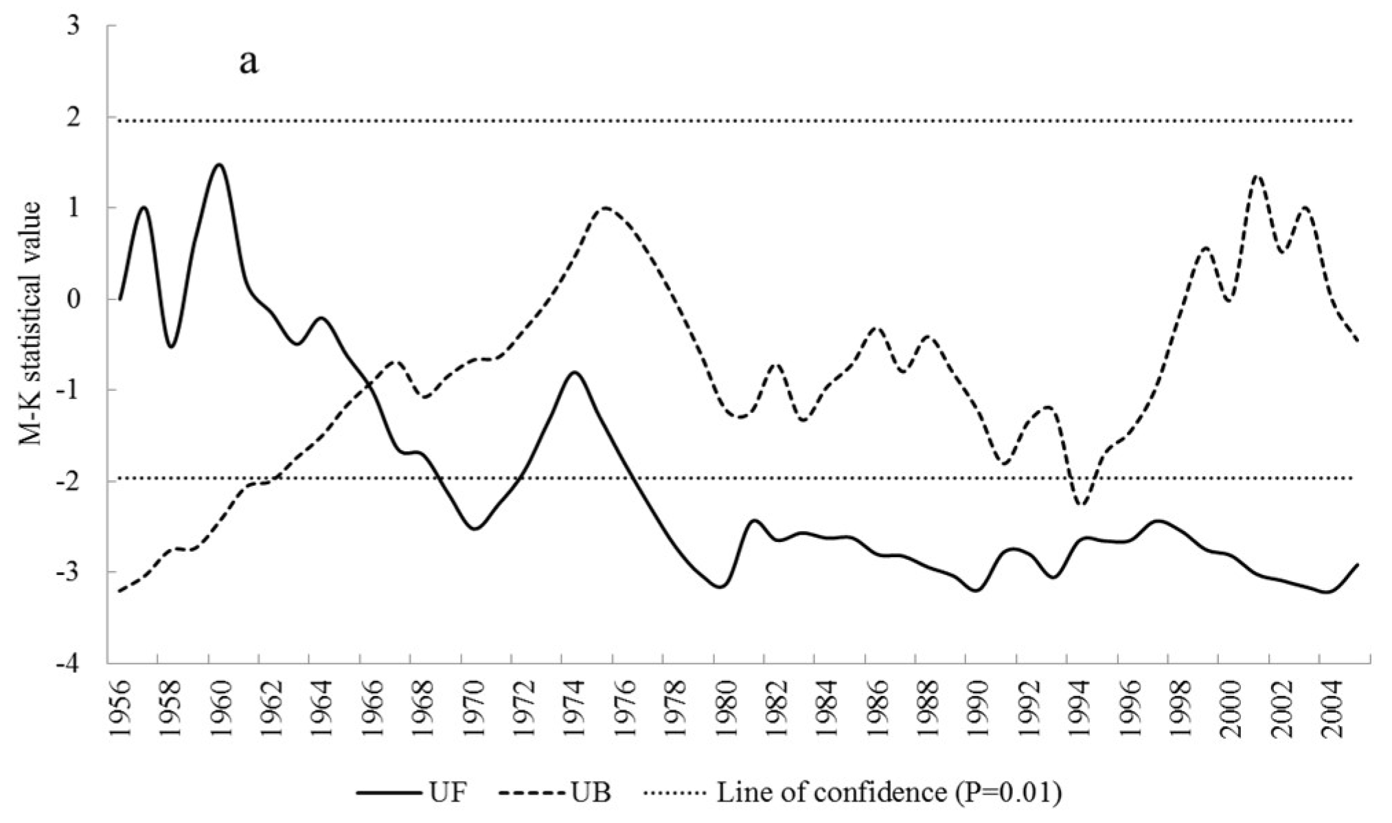
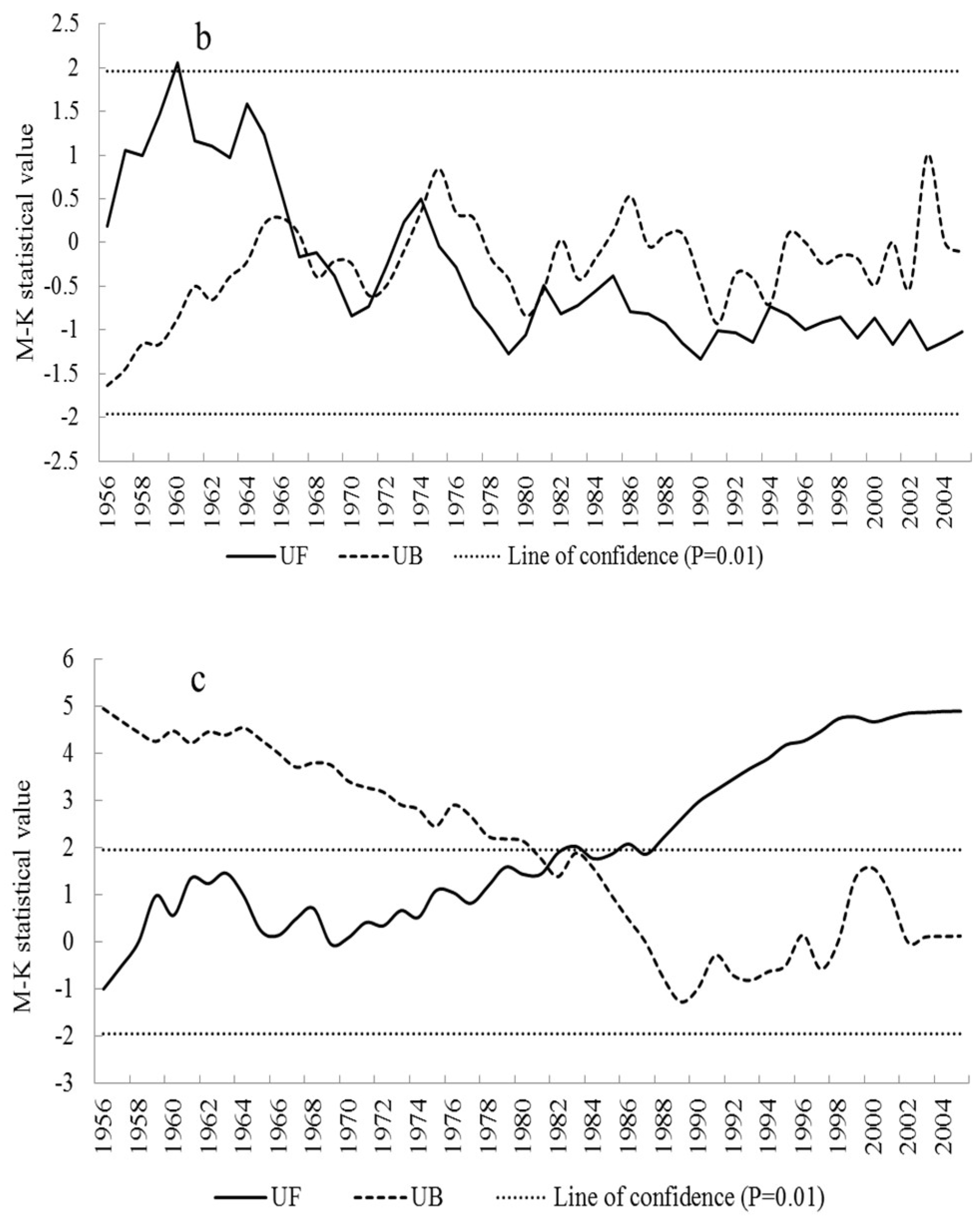
3.1. Hydro-Meteorological Data Analysis

The Mann–Kendall nonparametric test was used to investigate the possible trends of the hydrological processes and abrupt time series changes. Specifically, it analyzed the trends in the changes and the possible transition points of river runoff, temperature and precipitation. Climatic change was analyzed based on the annual precipitation and average annual temperature data from 1956 to 2005 in the upper Naoli River watershed (Figure 2, Table 1). The year 1966 was considered a jump point of runoff beginning to decrease (Figure 2a), which was similar with rain change (Figure 2b). However, the decreasing trend of rain was non-significant at the 95% confidence level, in both the 1956–1966 and 1967–2005 periods (Table 1). By contrast, the runoff of the upper Naoli River watershed decreased significantly during 1956–1966, with a test statistics value (Z) of −3.313 and an inclination value (β) of −2.670. The decreasing rate reduced during 1967–2005, with a Z value of −0.823 and a β value of −1.308. As shown in Figure 2c, the temperature of the Naoli River watershed increased on the whole during 1956–2005, having a Z value of 4.448 and a β value of 0.042. Moreover, the increasing trend was more significant after 1966, and the year 1983 was identified as the jump point. This showed that the trend of runoff change was consistent with that of runoff. Furthermore, an inverse correlation between the change trend of the runoff value and the temperature was identified.

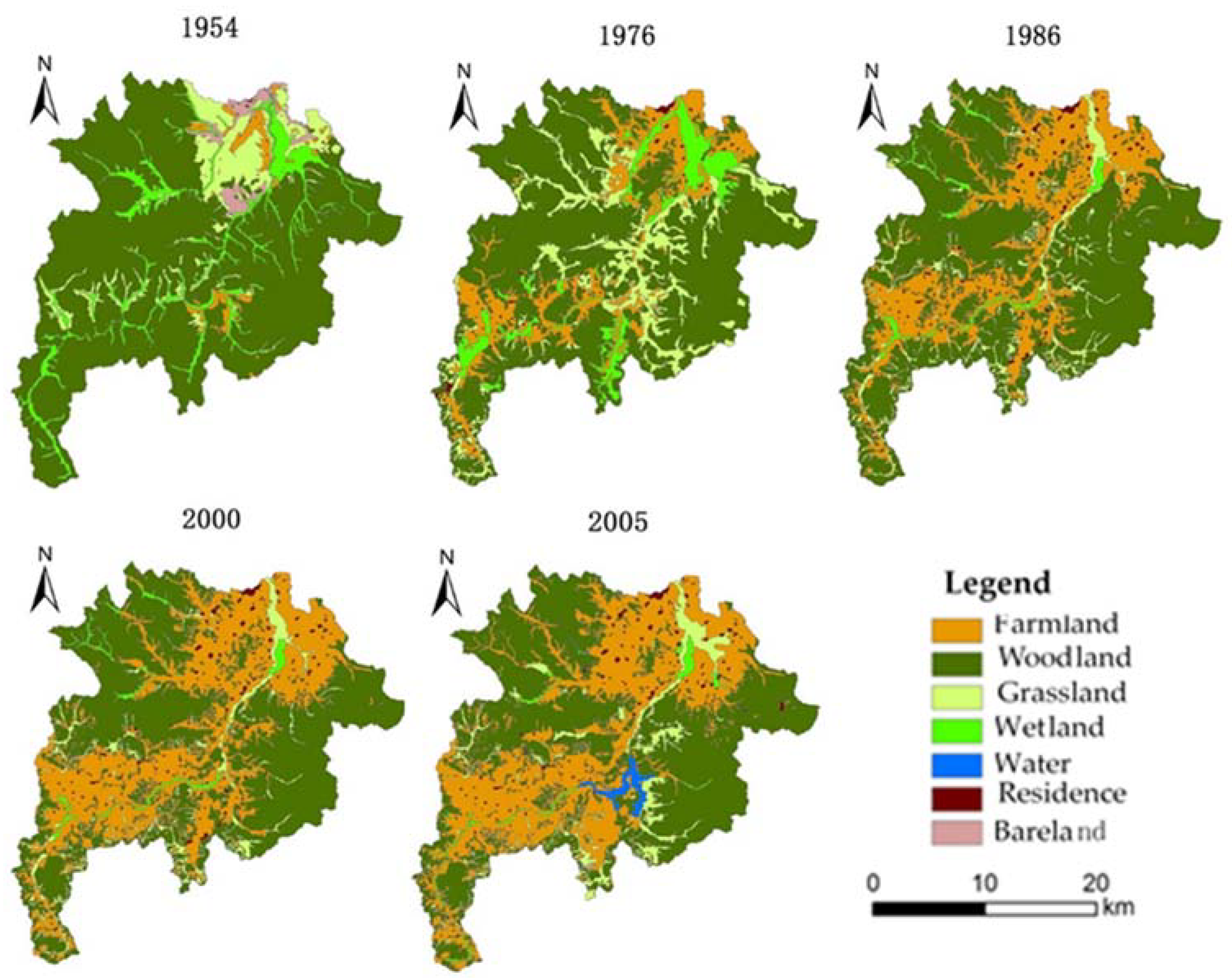
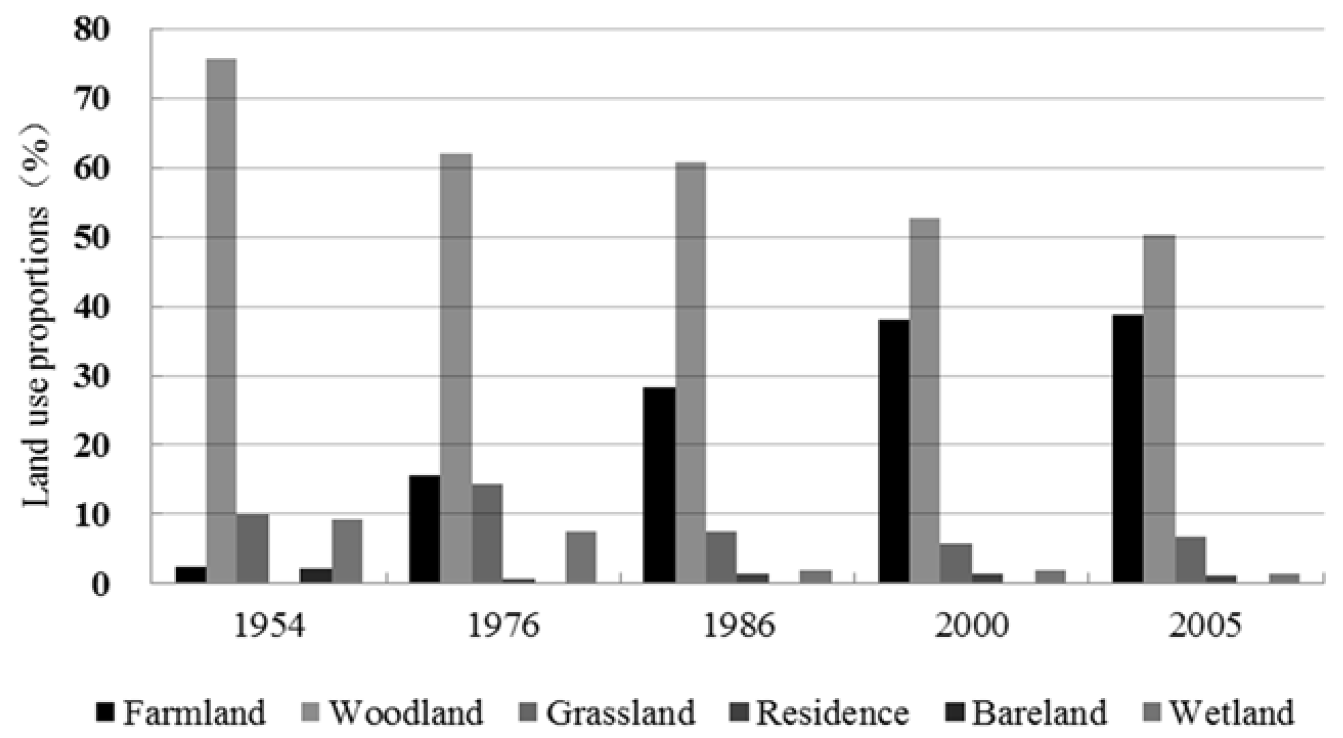
3.2. Landscape Change

In the basin in the 1950s, the main land use types were woodland, grassland, and wetland. Over the past 60 years, these land use types have been gradually decreasing, while the farmland area has been increasing (Figure 3 and Figure 4). In fact, the proportional extent of farmland increased from 2.54% to 38.78% from 1954 to 2005, with significant increases during the 1976–2005 period. Conversely, the proportional extent of woodland, grassland and wetland decreased from 75.70% to 50.21%, 10.00% to 6.91%, and 9.37% to 1.52%, respectively, during 1954–2005. Therefore, it may be inferred that the increase of arable land was mainly caused by the decrease of woodland, grassland and wetland areas.

3.3. Calibration and Validation Results

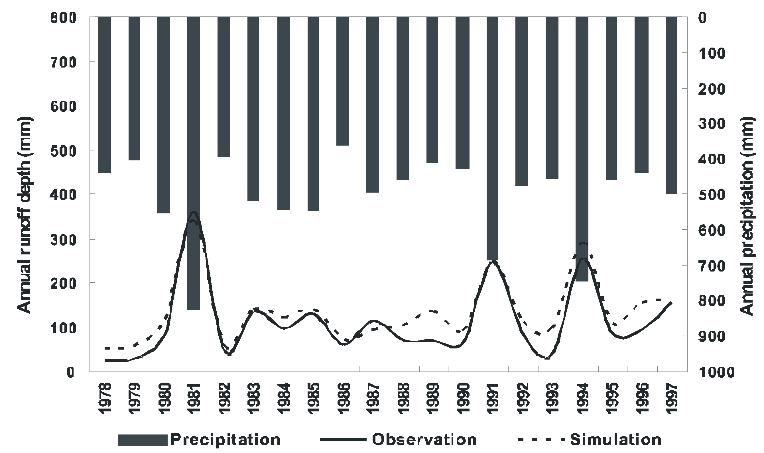
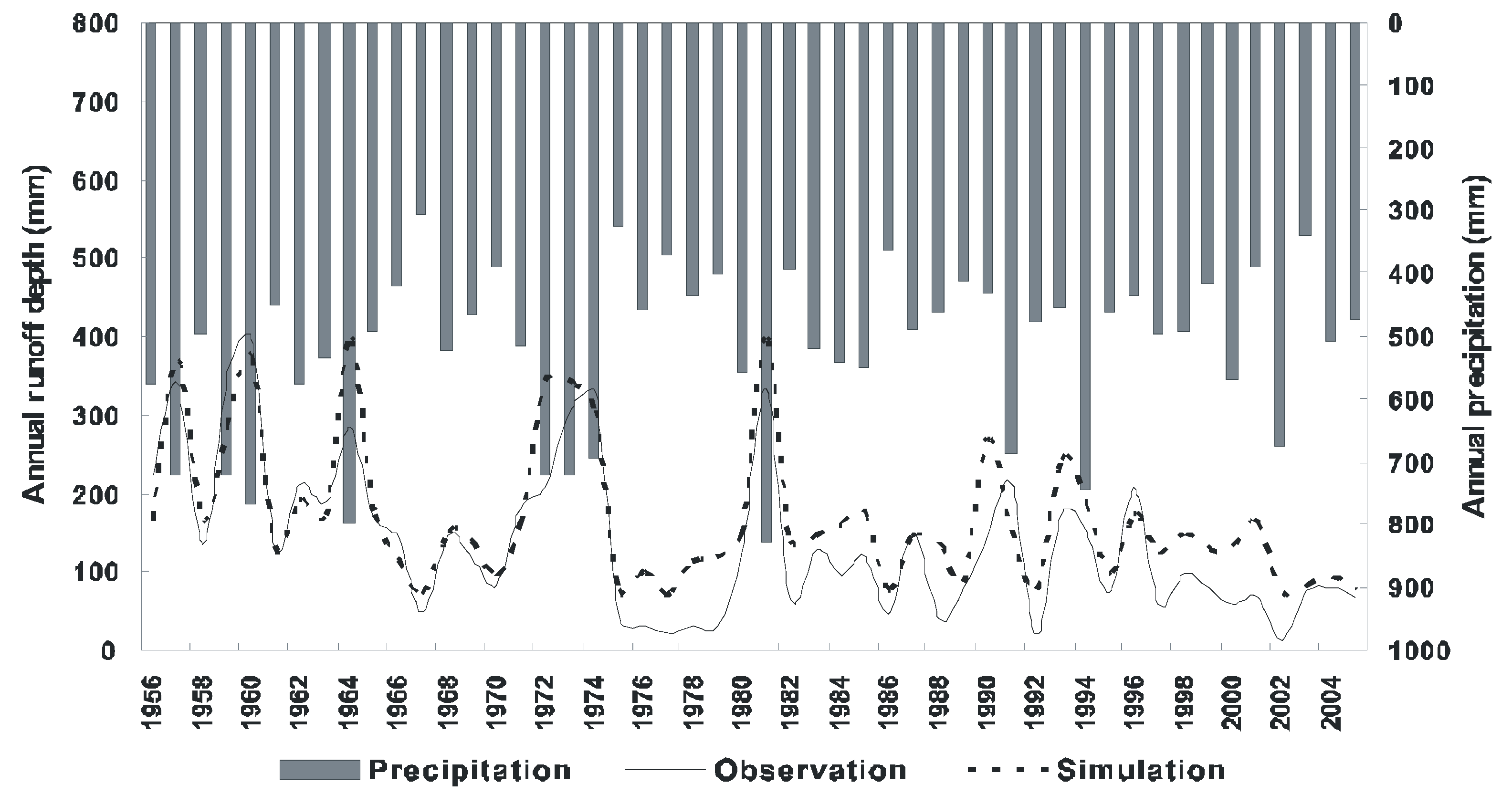
3.3.1. Model Calibration and Validation

Model calibration of SWAT was performed using 2000 land use maps to calibrate the annual streamflow from 1988 to 1997 at the outlet of Baoqing station. After model calibration, a simulation setup—employing the 1986 land use maps—was used to validate annual streamflow from 1978 to 1987 at Baoqing station. Model calibration was usually carried out by adjusting the values of the model parameters. The LH-OAT (Latin hypercube sampling based on one factor at a time) method was used for the sensitivity analysis, and SWAT-CUP (calibration and uncertainty programs) was used for calibration of the model runs. SWAT-CUP is a freeware program which allows the use of the different algorithms such as MCMC (markov chain monte carlo), GLUE (generalized likelihood uncertainty estimation), ParaSol (parameter solution) and SUFI-2 (sequential uncertainty fitting version 2) for optimization of the SWAT model [29,30]. According to the analysis, the relatively sensitive parameters for the hydrological components were CN2, ALPHA_BF, CANMX, ESCO, SURLAG, CH-K2, SOL_AWC and SOL_Z. The most sensitive parameter was CN2. The optimal values for SWAT calibration are listed in Table 2. The calibrated values were fine-tuned until the simulated results were acceptable according to the criteria used to evaluate model performance.
IHACRES was used to calibrate the annual streamflow from 1956 to 1966, and for validation during 1967 to 2005, at the outlet of Baoqing station. The division of the periods was based on the Mann–Kendall results of the annual runoff during 1956–2005 (Figure 2). The optimal values for the IHACRES model calibration are listed in Table 3.

3.3.2. Calibration and Validation Results

The results of the average annual streamflow simulated by the SWAT model and the IHACRES model are shown in Figure 5 and Figure 6, respectively. In the SWAT model, the watershed runoff was divided into two stages; that is, the period of calibration, 1988–1997, and the period of validation, 1978–1987. The IHACRES model was similarly divided, with the period of calibration being 1956–1966, and the period of validation being 1967–2005. The results showed that the observed and simulated runoff values followed the area rainfall patterns. A comparison of the observed and simulated runoff values showed good agreement, indicating that both the SWAT model and IHACRES model represented the observed runoff well in the upper Naoli River watershed. The NS, R2 and PBIAS values for annual calibration and validation are listed in Table 4. All NS and R2 values were above 0.7, and the absolute values of PBIAS were smaller than 25% disposed of one period in the validation period of the IHACRES model (Table 4), suggesting satisfactory model performance. During the calibration period, R2, NS and PBIAS values were 0.97, 0.89 and 0.17, respectively, for the SWAT model, and 0.78, 0.72 and −0.02, respectively, for the IHACRES model. In the validation period, R2, NS and PBIAS values were 0.97, 0.94 and 0.11, respectively, for the SWAT model, and 0.77, 0.70 and 0.26, respectively, for the IHACRES model. Thus, both models were capable of capturing long-term runoff yield in the upper Naoli River watershed.
Additionally, in order to compare the simulation effects of the two models, it was necessary to obtain the simulation results for the IHACRES model for the periods 1978–1997 and 1978–1987. The simulation results for the SWAT and IHACRES models are presented in Figure 7 as a tendency chart. Furthermore, the three performance evaluation criteria were also calculated for the IHACRES model over the two aforementioned periods. Table 4 outlines the R2, NS and PBIAS values for the SWAT model and IHACRES model over the different periods. For the IHACRES model, the R2, NS and PBIAS values were calculated as 0.73, 0.58 and −0.22, respectively, in 1988–1997, and 0.81, 0.62, and −0.35, respectively, in 1978–1987. The streamflow values simulated by the IHACRES model were bigger than the observed runoff values. By comparison, the fitting effect of the observed values and the simulated values were found to be better for SWAT model.
There were a few differences between the observed and simulated runoff values during specific years. The SWAT model, for example, had simulated values which were larger than the observed ones in 1978, 1979, 1989, 1993, 1996, and so on, as shown in Figure 5. In brief, the major discrepancies between the simulated and observed runoff were found in the dry and wet seasons. Specifically, the model overestimated dry season flow and underestimated the wet season flow.
As for the IHACRES model (Figure 6), a good match was found between the simulated and observed values in the calibration period of 1956–1966—except in 1964, when the simulated runoff was larger than the observed one. However, in the validation period, 1967–2005, the simulated values were larger than the observed ones on the whole.

4. Discussion

In this research, the simulation of streamflow variation—through use of both a SWAT model and IHACRES model—represented a new attempt to predict the hydrologic response in a marsh river. The underlying surface of the study area had changed significantly in the last 50 years. The land use types that were significantly reduced include the woodland, grassland and wetland areas. Studies have shown that forests can have an important role in soil and water conservation. The stream flow will also increase in the flood season and decrease in the low water period when forestland and pasture are reclaimed [31]. In addition, research has shown that a decrease in wetland area brings about a decrease of runoff depth [11,32]. For this study, the change in land use is considered another critical factor leading to runoff variation, besides the reason of rain change, particularly from 1976 to 2005.
The simulated runoff values were larger than the observed ones using the IHACRES model over the 1978 to 1997 period. This indicates that human activities, such as reclamation, has caused runoff reduction in the upper Naoli River watershed. Hou et al. [33] found that a vast expanse of natural wetlands were reclaimed blindly in the Naoli River basin. This change in underlying surface conditions caused the increase of evaporation and a reduction of runoff in the basin. In addition, the increased farmland irrigation area has brought about the increase of agricultural water consumption, and directly caused the decrease of runoff, according to Yao et al. [34].
The accuracy of the SWAT model was better than that of the IHACRES model for streamflow simulation in the upper Naoli River watershed. This was due to the construction defect of the IHACRES model, whereby only the meterologic elements were included, while other factors, such as human activity (e.g., land development), were lacking. While this study found that the impacts of human activities were minor during 1956–1966, with changes in the runoff appearing consistent with climate change, the impact of human activities led directly to runoff reduction between 1967 and 2005, when reclamation was prevalent in the area [9,35].
Overall, the IHACRES model was more suitable for runoff simulation in the basin during periods with minor human impact, because it had fewer types of input data and model parameters. Conversely, the SWAT model was more appropriate in periods with intensified human activity.

5. Conclusions

In this study, through the analysis of hydro-meteorological and land use data, the year 1966 was found to be a jump point of when rain began to decrease. The variation of rain was the primary cause for streamflow decreases observed during the 1956–1966 period, while the effects of human activities—such as land use change—were found to be the main cause during 1967–2005.
A comparison of the runoff simulation performance of a SWAT model and an IHACRES model was made in the upper Naoli River watershed, located in the center of the Sanjiang Plain, northeast China. The IHACRES model was easy to use with minimum input data and was suitable for runoff simulation in primeval times of the basin. In particular, it performed well during 1956–1966, while the simulated runoff values were larger than the observed ones during 1967–2005. The impacts of significant land use and climate changes, accompanied with a large-scale reclamation that occurred gradually after the 1950s, would be the main reason leading to runoff reduction. In addition, the simulation results of the IHACRES model for the period 1978–1997 were chosen for intercomparison with the SWAT model.
In contrast to the IHACRES model, the SWAT model could simultaneously simulate the water quantity and evaluate the impacts of climate variability and human activities, based on complex physical processes with plenty of input data. Also, the accuracy of the SWAT model was better than the IHACRES model for both the calibration and validation periods. This made the SWAT model a better tool for sustainable water resource management in the Naoli River watershed, where agricultural activities are intensive.

Author Contributions

G.L. conceived the manuscript; Z.H. provided support to model setup; Z.L. provided the data and related analysis; G.L. discussed the results and wrote the paper; S.Q. proofread the paper. All authors made revisions and improvements to the final version.

Funding

This study was funded by the auspices of National Natural Science Foundation of China (No. 41501026), Key project from Educational Department of Jiangxi province (GJJ160321), the Opening Fund of Key Laboratory of Poyang Lake Wetland and Watershed Research (Jiangxi Normal University), Ministry of Education (ZK2014003), Postdoctoral Science Foundation funded project of Jiangxi province (2014KY13).

Acknowledgments

The authors would like to express our thanks to the anonymous reviewers and the editors for useful ideas for improvement. Any errors and views expressed in this paper are the sole responsibility of the authors.

Conflicts of Interest

The authors declare no conflict of interest.

References

  1. Gao, C.Y.; Zhang, S.Q.; Liu, H.X.; Cong, J.X.; Wang, G.P. The impacts of land reclamation on the accumulation of key elements in wetland ecosystems in the Sanjiang Plain, northeast China. Environ. Pollut. 2018, 237, 487–498. [Google Scholar] [CrossRef] [PubMed]
  2. Wang, Z.M.; Mao, D.H.; Li, L.; Jia, M.; Dong, Z.Y.; Miao, Z.H.; Ren, C.Y.; Song, C. Quantifying changes in multiple ecosystem services during 1992–2012 in the Sanjiang Plain of China. Sci. Total Environ. 2015, 514, 119–130. [Google Scholar] [CrossRef] [PubMed]
  3. Yan, F.Q.; Zhang, S.W.; Liu, X.T.; Yu, L.X.; Chen, D.; Yang, J.C.; Yang, C.B.; Bu, K.; Zhang, L.P. Monitoring spatiotemporal changes of marshes in the Sanjiang Plain. China Ecol. Eng. 2017, 104, 184–194. [Google Scholar] [CrossRef]
  4. Jin, X.M.; Li, Y.; Fu, B.L.; Yin, S.B.; Yang, G.; Xing, Z.F. Spatiotemporal characteristics of wetland to farmland conversion processes in different geomorphological divisions during 1954–2015: A case study in the Sanjiang Plain north of the Wanda Mountains. Acta Ecol. Sin. 2017, 37, 3286–3294. (In Chinese) [Google Scholar]
  5. Liu, J.P.; Du, B.J.; Sheng, L.X.; Tian, X.Z. Dynamic patterns of change in marshes in the Sanjiang Plain and their influential factors. Adv. Water Sci. 2017, 28, 22–31. (In Chinese) [Google Scholar]
  6. Li, Z.Q.; Gan, Y.Q.; Zhou, A.G.; Liu, Y. Relationship between water discharge and sulfate sources of the Yangtze River inferred from seasonal variations of sulfur and oxygen isotopic compositions. J. Geochem. Explor. 2015, 153, 30–39. [Google Scholar] [CrossRef]
  7. Hu, Y.X.; Huang, J.L.; Du, Y.; Han, P.; Wang, J.L.; Huang, W. Monitoring wetland vegetation pattern response to water-level change resulting from the Three Gorges Project in the two largest freshwater lakes of China. Ecol. Eng. 2015, 74, 274–285. [Google Scholar] [CrossRef]
  8. Li, N.; Lei, G.P.; Zhang, H.; Zhou, H. Spatial-Temporal Characteristics of Farmland due to the Paddy Field Expansion in Naolihe River Basin. Res. Soil Water Conserv. 2016, 23, 63–73. (In Chinese) [Google Scholar]
  9. Wang, Z.; Song, K.; Ma, W.; Ren, C.; Zhang, B.; Liu, D.; Chen, J.M.; Song, C. Loss and fragmentation of marshes in the Sanjiang plain, northeast China 1954–2005. Wetlands 2011, 31, 945–954. [Google Scholar] [CrossRef]
  10. Liu, L.L.; Du, J.J. Documented changes in annual runoff and attribution since the 1950s within selected rivers in China. Adv. Clim. Chang. Res. 2017, 8, 37–47. [Google Scholar] [CrossRef]
  11. Liu, Z.M.; Lv, X.G.; Zhao, Y.B. Influence of Wetland and Farmland Changes on Runoff Depth in Naolihe River Basin. J. China Hydrol. 2009, 29, 93–96. [Google Scholar] [CrossRef]
  12. Zhang, L.; Karthikeyan, R.; Bai, Z.; Wang, J. Spatial and temporal variability of temperature, precipitation, and streamflow in upper Sang-kan basin, China. Hydrol. Process. 2018, 31, 279–295. [Google Scholar] [CrossRef]
  13. Ochoa-Tocachi, B.F.; Buytaert, W.; De Bièvre, B. Regionalization of land-use impacts on streamflow using a network of paired catchments. Water Resour. Res. 2016, 52, 6710–6729. [Google Scholar] [CrossRef] [Green Version]
  14. Giri, S.; Nejadhashemi, A.P.; Woznicki, S.A. Evaluation of targeting methods for implementation of best management practices in the Saginaw River Watershed. J. Environ. Manag. 2012, 103, 24–40. [Google Scholar] [CrossRef] [PubMed]
  15. Zhang, S.T.; Liu, Y.; Li, M.; Liang, B. Distributed hydrological models for addressing effects of spatial variability of roughness on overland flow. Water Sci. Technol. 2016, 9, 249–255. [Google Scholar] [CrossRef]
  16. Krogh, S.A.; Pomeroy, J.W.; Marsh, P. Diagnosis of the hydrology of a small Arctic basin at the tundra-taiga transition using a physically based hydrological model. J. Hydrol. 2017, 550, 685–703. [Google Scholar] [CrossRef]
  17. Boongaling, C.G.K.; Faustino-Eslava, D.V.; Lansigan, F.P. Modeling land use change impacts on hydrology and the use of landscape metrics as tools for watershed management: The case of an ungauged catchment in the Philippines. Land Use Policy 2018, 72, 116–128. [Google Scholar] [CrossRef]
  18. Gashaw, T.; Tulu, T.; Argaw, M.; Worqlul, A.W. Modeling the hydrological impacts of land use/land cover changes in the Andassa watershed, Blue Nile Basin, Ethiopia. Sci. Total Environ. 2017, 619–620, 1394–1408. [Google Scholar] [CrossRef] [PubMed]
  19. Vansteenkiste, T.; Tavakoli, M.; Steenbergen, N.V.; Smedt, F.D.; Batelaan, O.; Pereira, F.; Willems, P. Intercomparison of five lumped and distributed models for catchment runoff and extreme flow simulation. J. Hydrol. 2014, 511, 335–349. [Google Scholar] [CrossRef]
  20. Soulis, K.X.; Valiantzas, J.D.; Ntoulas, N.; Kargas, G. Simulation of green roof runoff under different substrate depths and vegetation covers by coupling a simple conceptual and a physically based hydrological model. J. Environ. Manag. 2017, 200, 434–445. [Google Scholar] [CrossRef] [PubMed]
  21. Masafu, C.K.; Trigg, M.A.; Carter, R.; Howden, N.J.K. Water availability and agricultural demand: An assessment framework using global datasets in a data scarce catchment, Rokel-Seli River, Sierra Leone. J. Hydrol. Reg. Stud. 2016, 8, 222–234. [Google Scholar] [CrossRef]
  22. Neitsch, S.L.; Arnold, J.G.; Kiniry, J.R.; Williams, J.R. Soil and Water Assessment Tool; version 2005; Theoretical Documentation; USDA-ARS: Temple, TX, USA, 2005.
  23. Arnold, J.G.; Srinivasan, R.; Muttiah, R.S.; Williams, J.R. Large area hydrologic modeling and assessment (Part I): Model development. J. Am. Water Resour. Assoc. 1998, 34, 73–89. [Google Scholar] [CrossRef]
  24. Jakeman, A.J.; Glittlewood, L.; Whitehead, P.G. Computation of the instantaneous unit hydrograph and identifiable component flows with application to two small upland catchments. J. Hydrol. 1990, 117, 275–300. [Google Scholar] [CrossRef]
  25. Dye, P.J.; Croke, B.F.W. Evaluation of streamflow predictions by the IHACRES rainfall-runoff model in two South African catchments. Environ. Model. Softw. 2003, 18, 705–712. [Google Scholar] [CrossRef]
  26. Kim, K.B.; Kwon, H.; Han, D. Exploration of warm-up period in conceptual hydrological modelling. J. Hydrol. 2018, 556, 194–210. [Google Scholar] [CrossRef]
  27. Moriasi, D.N.; Arnold, J.G.; Van Liew, M.W.; Bingner, R.L.; Harmel, R.D.; Veith, T.L. Model evaluation guidelines for systematic quantification of accuracy in watershed simulations. Trans. ASABE 2007, 50, 885–900. [Google Scholar] [CrossRef]
  28. Herman, M.R.; Nejadhashemi, A.P.; Aboualid, M.; Hernandez-Suarez, J.S.; Daneshvar, F.; Zhang, Z.; Anderson, M.C.; Sadeghi, A.M.; Hain, C.R.; Sharifi, A. Evaluating the role of evapotranspiration remote sensing data in improving hydrological modeling predictability. J. Hydrol. 2018, 556, 39–49. [Google Scholar] [CrossRef]
  29. Abbaspour, K.C. SWAT-CUP 2012: SWAT Calibration and Uncertainty Programs—A User Manual; Eawag Aquatic Research: Dübendorf, Switzerland, 2015. [Google Scholar]
  30. Abbaspour, K.C.; Yang, J.; Maximov, I.; Siber, R.; Bogner, K.; Mieleitner, J.; Zobrist, J.; Srinivasan, R. Modelling hydrology and water quality in the pre-alpine/alpine Thur watershed using SWAT. J. Hydrol. 2007, 333, 413–430. [Google Scholar] [CrossRef]
  31. Lin, B.Q.; Chen, X.W.; Yao, H.X.; Chen, Y.; Liu, M.B.; Gao, L.; James, A. Analyses of landuse change impacts on catchment runoff using different time indicators based on SWAT model. Ecol. Indic. 2015, 58, 55–63. [Google Scholar] [CrossRef]
  32. Liu, X.T. Water storage and flood regulation functions of marsh wetland in the Sanjiang Plain. Wetl. Sci. 2007, 5, 64–68. [Google Scholar]
  33. Hou, W.; Zhang, S.; Zhang, Y.; Kuang, W. Analysis on the shrinking process of wetland in Naoliriver Basin of Sanjiang Plain since the 1950s and its driving forces. J. Nat. Resour. 2004, 19, 725–731. (In Chinese) [Google Scholar]
  34. Yao, Y.; Lv, X.; Wang, L. Tendency and periodicity of annual runoff of Naoli River from 1956 to 2005. Resour. Sci. 2009, 31, 648–655. (In Chinese) [Google Scholar]
  35. Liu, X.T.; Ma, X.H. Influence of large-scale reclamation on natural environment and regional environmental protection in the Sanjiang plain. Sci. Geogr. Sin. 2000, 20, 14–19. (In Chinese) [Google Scholar]
Figure 1. Location of the upper Naoli River catchment.
Water 10 01004 g001
Figure 2. Mann–Kendall results of: (a) Annual runoff; (b) precipitation; and (c) temperature, in the upper Naoli River watershed during 1956–2005.
Water 10 01004 g002aWater 10 01004 g002b
Figure 3. Charts of land use in the upper Naoli River watershed during 1954–2005.
Water 10 01004 g003
Figure 4. Changes in the proportional extent for five land use classes in the upper Naoli River watershed.
Water 10 01004 g004
Figure 5. Annual precipitation and simulated and observed runoff depth using the SWAT model in the upper Naoli River watershed, during 1978–1997.
Water 10 01004 g005
Figure 6. Annual precipitation and simulated and observed runoff depth using the IHACRES model in the upper Naoli River watershed, during 1956–2005.
Water 10 01004 g006
Figure 7. Comparison of observed and simulated annual runoff between the SWAT and IHACRES models in the upper Naoli River Watershed, during 1978–1997.
Water 10 01004 g007
Table 1. Statistic values of runoff and meteorological elements in the upper Naoli River watershed.
Meteorologic and Runoff Elements1956–19661967–2005
ZβH0ZβH0
Rain (mm)−1.640−1.780Accept0.073−0.862Accept
Temperature (°C)4.4480.042Reject2.9150.036Reject
Runoff depth (mm)−3.313−2.670Reject−0.823−1.308Accept
Table 2. Description, default and optimal values used in the model calibration/validation of the SWAT (soil and water assessment tool) model.
ParameterDescriptionDefaultOptimal Value
CN2SCS runoff curve number for moisture condition II60–8770–102
ALPHA_BFBase flow recession constant0.0480.17
ESCOSoil evaporation compensation factor0.950.97
CANMXMaximum canopy storage01.38
SOL_AWCAvailable water capacity of the soil layer0.13–0.180.16–0.22
SOL_ZDepth from soil surface to bottom of layer120–250128–267
SURLAGSurface runoff lag time41.16
CH-K2Effective hydraulic conductivity in main channel alluvium058.44
Table 3. Description, default and optimal values used in the model calibration/validation of the IHACRES (identification of unit hydrographs and component flows from rainfall, evapotranspiration and streamflow data) model.
ParameterDescriptionDefaultOptimal Value
wDrying rate at reference temperature2–302
fTemperature dependence of drying rate0–42.1
cA parameter calculated so that the volume of effective rainfall is equal to the total flow for the calibration period00.056
trReference temperature2017
δTime delay for flow response10
Table 4. Statistical comparison of the observed and simulated annual runoff in the upper Naoli River watershed.
ModelPeriodsPerformance Evaluation Criteria
R2NSPBIAS
SWAT1988–19970.970.890.17
1978–19870.970.940.11
IHACRES1956–19660.780.72−0.02
1967–20050.770.700.26
1988–19970.730.58−0.22
1978–19870.810.62−0.35

