1. Introduction
The morphodynamical evolution of rivers is a challenging and topical task that can affect many aspects of the economy of the surrounding region, such as the navigability of the river or the safety of the plantations, industries and villages located just behind the banks.
This fascinating topic involves different features of river dynamics, such as water flow, sediment transport and changes in channel morphology, comprehending both bed and banks evolution [
1]. In fact, many rivers can display morphological adjustments not only in the shape of the cross section, but also in the river width or in its planform, if they are not rigidly constrained between a fixed embankment and if geological conditions allow for it [
2].
In particular, lower river courses are often characterized by a very small longitudinal slope [
3,
4], which facilitates instability phenomena [
5], generating meanders [
6], which tend to deform and migrate [
7,
8], in the context of the morphological evolution of the river [
9]. Some studies analyse meander development and instability from an analytical point of view [
10,
11,
12,
13] or they search for an equilibrium solution under certain conditions [
14]. Others focus on the local curvature-induced effects [
15], which generate a secondary current, consisting in an outwards motion near the water surface and an inwards motion at the bottom, perpendicular to the main flow [
8]. This helical motion emphasizes the three-dimensional nature of the flow and enhances the stresses near the outer bank [
16], responsible for meander formation and migration. Moreover, this has also been confirmed by experimental investigations, which have recently also highlighted the presence of a counter-rotating circulation cell near the outer bank, which could influence the bank shear stress distribution [
17]. The effect of secondary currents is particularly evident in the bed load transport [
18,
19], creating a particular morphology given by the longitudinal sequence of laterally adjacent erosion and accretion zones [
20].
Nevertheless, theoretical approaches are not always well-suited to investigate case studies, where several different parameters are needed and hence a simple and adaptable instrument is more advisable. Numerical models based on three-dimensional equations would be able to describe the three-dimensional flow structures caused by the meander morphology more adequately, nevertheless they are too heavy from a computational point of view to be applied to large natural environments, such as natural rivers. Bidimensional models (2DH models) work on depth integrated variables and hence they are not suitable to describe strongly three-dimensional flow structures or local phenomena such as the pattern of the fluid over the dunes, which strongly influences the shape and dimension of the bedforms [
21]. However, 2DH models can give a useful general interpretation of the river evolution, without the pretension of capturing localized phenomena.
In light of this, bidimensional numerical models integrated over water depth are revealed to be a valuable and low-cost tool in addressing this issue and their use is becoming more common, thanks to increasing computer power and parallel computing techniques.
In the literature, several models have been presented on this topic. Some of them focus their attention on the influence of secondary currents on river bends, for example adding dispersive terms to momentum and transport equations (e.g., [
22,
23,
24]). Nevertheless, they often work with fixed bed only [
24] or, if they consider changes in bed height, they do not simulate processes of bank erosion or deposition [
22,
23]. In this way, they are able to describe bed evolution, but cannot appreciate the morphological changes associated with the meandering. In fact, to face a similar problem, a specific technique to study the retreat of the banks is needed.
Bankline recession can be generated by several phenomena, among which hydraulic erosion plays a key role [
25]. This type of erosion can be regarded as the combination of two separate mechanisms, which are bounded and strongly interact with one another, even if they are controlled by different aspects [
26,
27]. The former is the flow-induced erosion, which causes the removal of sediment from the bank slope and a scour at the bank toe; this process triggers mass instability and hence it induces the local slump of blocks of bank material, which is indeed the latter mechanism. In turn, the failed sediments are entrained by the current, if flow conditions allow for it.
Following this line, most of the models which address the morphological evolution of the rivers couple hydrodynamic and bed evolution submodels with a bank erosion submodel, so they are able to predict changes in both bed and bank form, comprehending also bank failure (e.g., [
28,
29,
30,
31,
32,
33,
34,
35,
36,
37]). Nevertheless, their approach can differ significantly from one another.
One of the main distinctive traits is the way the bank erosion process is handled. Some authors, for example, conduct a proper bank stability investigation, considering a limit equilibrium analysis for planar or rotational slip failure [
29,
30] or a cantilever failure [
30]. Others evaluate a bank erosion/accretion rate, which gives rise to the displacement of bank top and a consequent mesh modification [
31,
32,
35,
36,
37] or, in a similar way, they couple a bed scouring with an intermittent bank erosion model, which shift the bank while keeping the same initial angle of repose [
28]. Another approach consists in coupling the basal erosion due to hydrodynamic forces with a bank failure model, which triggers when the bank slope exceeds a critical angle [
33,
34,
38,
39]. The wide variety of strategies adopted in literature indicates that the issue is still not a closed one.
Moreover, a few authors adopt a moving boundary fitted coordinate system that on the one hand simplifies the grid generation process, but on the other hand it needs a reshaping of the mesh at every shift of the bankline. The treatment of secondary currents has also been very well discussed, their influence depending on the magnitude of the curvature of the meander: some authors consider secondary currents in the hydrodynamics only or in the sediment transport only or they neglect them completely.
Even if it is recognized that flood waves play an important role in the dynamic of transport processes [
40], some models do not consider a complete unsteady flow evolution, restricting the hydrodynamic model to a steady formulation or they even neglect time-dependent channel width adjustments, assuming the river width as a constant. In the authors’ opinion, here the evolution of a meander cannot be observed by simulating a single flood event, but it is worth reproducing at least a few years of discharge to appreciate the bankline movement.
Finally, particular care should also be paid to the characterization of the sediments: most of the sediment transport numerical models deal with granular sediments only [
28,
34] and some of them even neglect the suspended sediments in favour of bed load [
22]. This may not be realistic in lower river courses, where the banks are often formed by a mix of sand and cohesive material [
26]. Many studies show that the incipient motion of cohesive sediments is much more complex to describe compared to the behaviour of granular sediments and it cannot be treated in the same way [
41,
42]. For example, the results of experiments show great uncertainty in the estimate of erosion thresholds [
42,
43,
44], which is a key parameter in the evaluation of sediment entrainment when an excess shear stress formula is used [
43,
45].
In the present paper, a fully unsteady finite volume 2DH morphodynamic model is presented, which couples the hydrodynamic flow with granular and cohesive sediment transport, treated separately. The bed height evolution is evaluated through the sediment continuity equation and a new local simple failure operator is inserted to allow bankline shifting, also in the presence of cohesive material, when bank slopes are usually very steep. Secondary flow effects on bed load are also considered. The numerical integration scheme is based on an accurate shock-capturing and C-property preserving approach, also able to describe shock phenomena properly [
46]. The model has been developed to apply it to real complex territorial domains to simulate a mid-length period of some years to study a meander evolution. Therefore, the authors have opted for a balance between accuracy and simplicity, trying to reduce the calibration parameters as much as possible. The resulting model is an agile tool, suitable to study the morphological changes of lowland rivers, where granular and cohesive sediments coexist. Finally, the developed model has been applied to a case study, represented by the final reach of the Tagliamento River in northern Italy. In particular, the analysis focuses on morphodynamic evolution of the last meander upstream of the mouth, which has been undergoing a strong evolution over the last few decades, probably caused by human intervention, that modified its planar course in the last century. In
Section 2, the governing equations are briefly recalled and the numerical technique is described. In
Section 3, the Tagliamento River case study is presented and the numerical results are discussed.
2. Numerical Model
The model presented in this paper is based on the shallow water hypothesis, assuming a hydrostatic pressure distribution over the water depth. The resulting hydrodynamic equation system can be written as:
with:
In these equations, (
t,
x,
y) are temporal and horizontal spatial coordinates and
U the variable vector, with
h the water depth and (
U,
V) the mean velocity over the depth in
x- and
y-directions. (
F,
G) and (
Ft,
Gt) are the vectors of advective and turbulent fluxes, with
g the gravity acceleration and
υt the horizontal eddy viscosity coefficient evaluated by means of a Smagorinsky approach as in [
47].
S is the source term vector, with
the water density and
zb the bottom height. (
τbx,
τby) are the components along
x and
y of the bed shear stress
τb, evaluated through Manning formula as:
nM being the Manning coefficient. In the present model, the effects of secondary currents on the hydrodynamic equations have not been considered. Moreover, assuming a hydrostatic pressure distribution, local effects related to vertical velocities and vertical accelerations cannot be appreciated; thus, some bedforms cannot be properly described.
The numerical modelling of the morphological evolution of the final reach of a river cannot leave out of consideration the presence of both granular and cohesive sediments. The former is further split into bed and suspended load. In the literature, bed load is usually treated with an equilibrium approach, while the suspended load can be addressed using both the equilibrium and non-equilibrium approach. Due to the results obtained in a previous test campaign [
48], the non-equilibrium approach is preferred for the suspended load of both granular and cohesive sediments in the present paper. This requires two additional depth-averaged advection–diffusion equations to study the concentration distribution of the suspended load:
where the subscript
i refers to granular (
g) or cohesive (
c) material,
Ci is the depth-averaged volume concentration of suspended sediment, and (
E −
D)
i represents the volume erosion
E or deposition rate
D of the suspended load.
The granular source-sink term of transport and sediment continuity equation (
E −
D)
g is evaluated as [
49]:
ws,g being the sediment fall velocity evaluated as in [
50],
ca the equilibrium concentration at the reference height
a, considered to be the upper end of the bed load layer, and
c0,g the actual concentration at the same height.
ca is evaluated as in [
51], while
c0,g is calculated from depth average sediment concentration
Cg assuming the vertical concentration profile proposed by [
50].
In the cohesive source/sink term, the erosion and deposition rates are evaluated separately from mass erosion and deposition rates (
Ecm and
Dcm, respectively) as:
with
ρs the grain density of cohesive material. In particular,
Ecm is based on an excess shear stress formula by Partheniades [
52]:
MPar and
nPar being two coefficients (in the following, 0.001 kg/(m
2s) and 1, respectively) and
τe the critical erosion bed shear stress. The critical bed shear stress is linked to the dry density
ρd through Thorn and Parson formula.
Dc is calculated following Krone’s theory [
45,
53]:
ws,c being the settling velocity as in [
43],
τd the critical bed shear stress for deposition and
c0,c the bed concentration of cohesive material, evaluated from depth average sediment concentration
Cc assuming the vertical concentration profile proposed by [
54].
The bed level change is evaluated by means of the sediment continuity equation, written separately for granular and cohesive material on a control volume near the river bed:
n being sediment porosity and
qb bed load transport, evaluated as in [
51] and corrected with a longitudinal and transverse bed slope factor [
51,
55].
As already stated, in the present paper, the helical flow has been considered as a further bed load component
qbs transverse to the flow direction, which is then added to
qb:
where
δs is the deflection angle of the bed shear stress from the main flow, evaluated following [
56,
57].
The total bed level change is due to the sum of the two contributes:
Equations (1), (6) and (11) are integrated over time with a Strang splitting scheme and in space with a finite volume method over a quadrangular irregular mesh, able to follow the river flow and banks as far as possible and at the same time flexible enough to describe sudden changes in the topography. The finite volume scheme adopted is based on Harten–Lax-van Leer–Contact (HLLC) Riemann solver [
58]. The intercell fluxes are first computed with a first-order method, from cell centered values of the variable, applying a hydrostatic variable reconstruction, which makes it possible to consider the source term due to bed slope as being distributed to the cell interfaces and hence as a correction to the intercell fluxes [
59]. The second-order extension consists in computing the fluxes from minmod-limited reconstructed values on both sides of each cell interface [
58]. In this way, the first-order technique can be applied, considering a further source term arising from the linear reconstruction of bottom height, which can also be distributed as before at the interfaces [
59]. Particular care has been devoted to variable reconstruction in case of wet and dry fronts, where the techniques introduced by [
60] are applied. This procedure assures the scheme is well balanced also in wet and dry conditions. The turbulent fluxes and the bed load at the intercell are evaluated by means of a centred finite difference scheme. The resulting scheme is second-order accurate both in space and time.
The granular sediment transport model has been applied to laboratory benchmark tests to check and compare different computational methods for bed and suspended loads [
46,
48,
61]. The cohesive sediment transport model has been successfully applied to the Marano and Grado Lagoon to verify the silting of navigable channels [
62].
Thus far, the model would not be able to represent changes in channel morphology because the bed erosion is strictly related to bed shear stress or sediment concentration, which vanish on dry bed. Thus, a dry land side would never be eroded, with consequent lack of bank retreat description. To avoid this deficiency, a local failure operator has been inserted to address the bankline failure topic.
As already stated, the bankline recession is due to the mutual interaction of two different mechanisms: the flow-induced lateral erosion and the geotechnical instability phenomena. From this perspective, the developed local failure operator consists of two processes; the former is a flow-induced erosion, with the consequent collapse of the resulting cantilever block, and the latter is an avalanching mechanism triggered by a geostatic bank instability. The sediments eroded by the flow and the failed material are relocated to the toe of the bank and they can be entrained by the current and hence removed in the follow-up of the simulation, if flow conditions allow for it. In this way, the resulting failure criterion guarantees the overall sediment mass conservation, a fundamental point when a river bank erosion predictor is included in a morphodynamic model [
63].
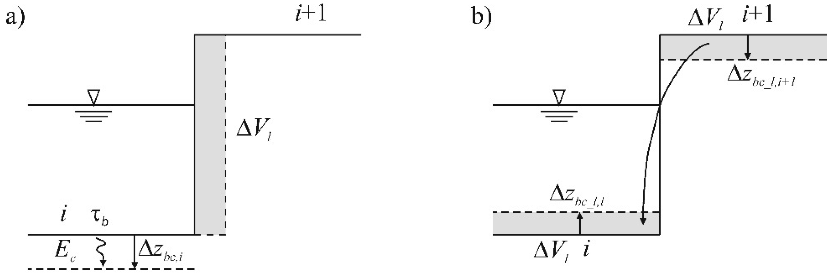
2.1. Flow-induced Erosion
The emerged portion of a cohesive bank can be very steep, e.g., the situation sketched in
Figure 1, where we can see the last wet cell of the river and first dry one of the bank, separated by a vertical wall (cell
i and
i + 1 in
Figure 1a, respectively). Here, the hydrodynamic flow causes not only the bed shear stress
τb on the wet cell, but also a lateral shear stress
τl, acting on the steep slope.
τb is involved in Equation (9) for the determination of the erosion rate
Ecm. If we assume that the bed shear stress exceeds
τe, the consequent bed erosion over a single time step Δ
t follows from Equation (11) as:
In a similar way, the bank undercutting can be related to the excess of shear stress
τl above a critical value, evaluating the lateral erosion rate
El (
Figure 1a), following Partheniades’ formula:
The lateral erosion drives the removal of a volume Δ
V1 from the bank face, but at the same time it also triggers the mass instability volume Δ
V2, as depicted in
Figure 1b. This situation will lead to a cantilever failure, caused by the weight of the cantilever block and emphasized by the weakening of soil resistance due to repeated cycles of wetting and drying [
26]. Thus, at the end of the lateral erosion process, the whole volume Δ
Vl, sum of Δ
V1 and Δ
V2, will fall producing the bank retreat (
Figure 2a). Working with a fixed mesh, this lateral erosion cannot be reproduced, unless the mesh is reshaped at every time step. As a solution, in the present model a new approach has been developed to consider the lateral erosion of the dry cell
i + 1 and it is depicted in
Figure 2b. First, the volume Δ
Vl that should be eroded by
El in a time step is evaluated as:
Ω
lat being the surface of the vertical wall. This volume is then removed from the bottom of cell
i + 1 and relocated on the bottom of cell
i. This causes an additional deposition/erosion on cell
i and
i + 1, due to the presence of the lateral shear stress:
Ω
i and Ω
i+1 being the bottom surface of cell
i and
i + 1. The sign is positive on the evaluation of cell
i, because there is a deposition and negative on cell
i + 1 because there is some erosion. These quantities should be added to the bottom variation due to the bed shear stress τ
b. Finally, the overall bed level change of the cohesive material for cells
i and
i + 1 can be evaluated as:
The lateral shear stress τl is here assumed to be equal to bed shear stress τb.
2.2. Geostatic Bank Failure
In addition to the phenomena related to lateral erosion, river banks can undergo geotechnical instability, due to submergence, which causes a reduction of the angle of repose. In this context, Spinewine et al. [
64] proposed two stability angles, one for submerged and the other for emerged material, highlighting that banks over the surface level can reach very high steep slopes, up to vertical values. On the other hand, the stability angle under the surface level can assume different values, depending on the authors (e.g., [
65,
66]). When the slope becomes steeper, for example due to a scour at the bank toe, the sediments begin to slide, forming a new slope. One possible approach is to make slipped material undergo a transition from bed layer to flow current, as suspended load [
39]. In the present paper, on the other hand, it has been decided to move the slipped material to the toe of the bank [
38], where it can be entrained by the current at a later time. In light of these considerations, a simple avalanching algorithm for submerged cells, based on the one-dimensional Larson model [
67], is here presented and extended to a bi-dimensional domain.
Following Allen [
68], two different limiting slopes are recognized: the angle of repose or the angle of initial yield
φi and the residual angle
φr. The former represents the critical value beyond which avalanching occurs and the material is redistributed along the slope; the latter is the final angle that the slope will reach at the end of the sliding process. In this way, slope steepness is limited to the repose angle.
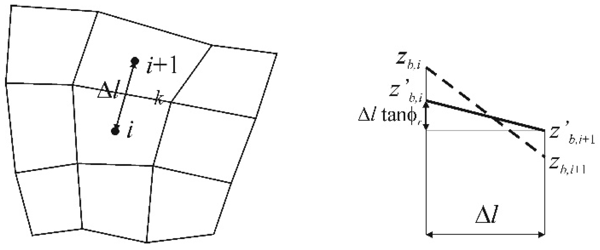
The cells being quadrangular, four different slopes can be identified between a cell and its neighbours. With reference to
Figure 3 and cell
i, it is possible to consider that the slope across side
k exceeds the critical value
φi and without loss of generality we can assume that z
b,i > z
b,i+1. The aim is to reduce z
b,i to z’
b,i and to increase z
b,i+1 to z’
b,i+1 to obtain the desired slope
φr, obviously conserving the mass of moved sediments. This can be written as:
Δ
l being the distance between cell
i and
i + 1 and Ω
i and Ω
i+1 the surface of cells
i and
i + 1. The final result is:
Should avalanching take place, it must be verified that all elements surrounding the modified cells are stable; in this way, the bottom height correction is recursive, until the desired slope is reached in the whole computational domain.
3. The Tagliamento River: Site Description and Field Data Collection
The present model has been applied to study the morphological evolution of the last meander of the Tagliamento River, located in northern Italy. The Tagliamento is a 180 km long river, flowing into the Adriatic Sea, with a catchment basin of 2870 km2. From the source in the Alps to the central part of its course, the bed is fully braided, while the river changes in its lower course to a single channel with lower longitudinal bottom slope and finer grained sediments. Following the river course downstream, the slope further decreases and some meanders are encountered.
In particular, the last reach of the river, just upstream of the mouth, has revealed substantial morphological changes over the last few decades, related to the strong interaction of several factors including floods, wave motion, tides and not least, human intervention. In fact, a morphological response to a technical action can activate the beginning of a channel evolution from an equilibrium configuration [
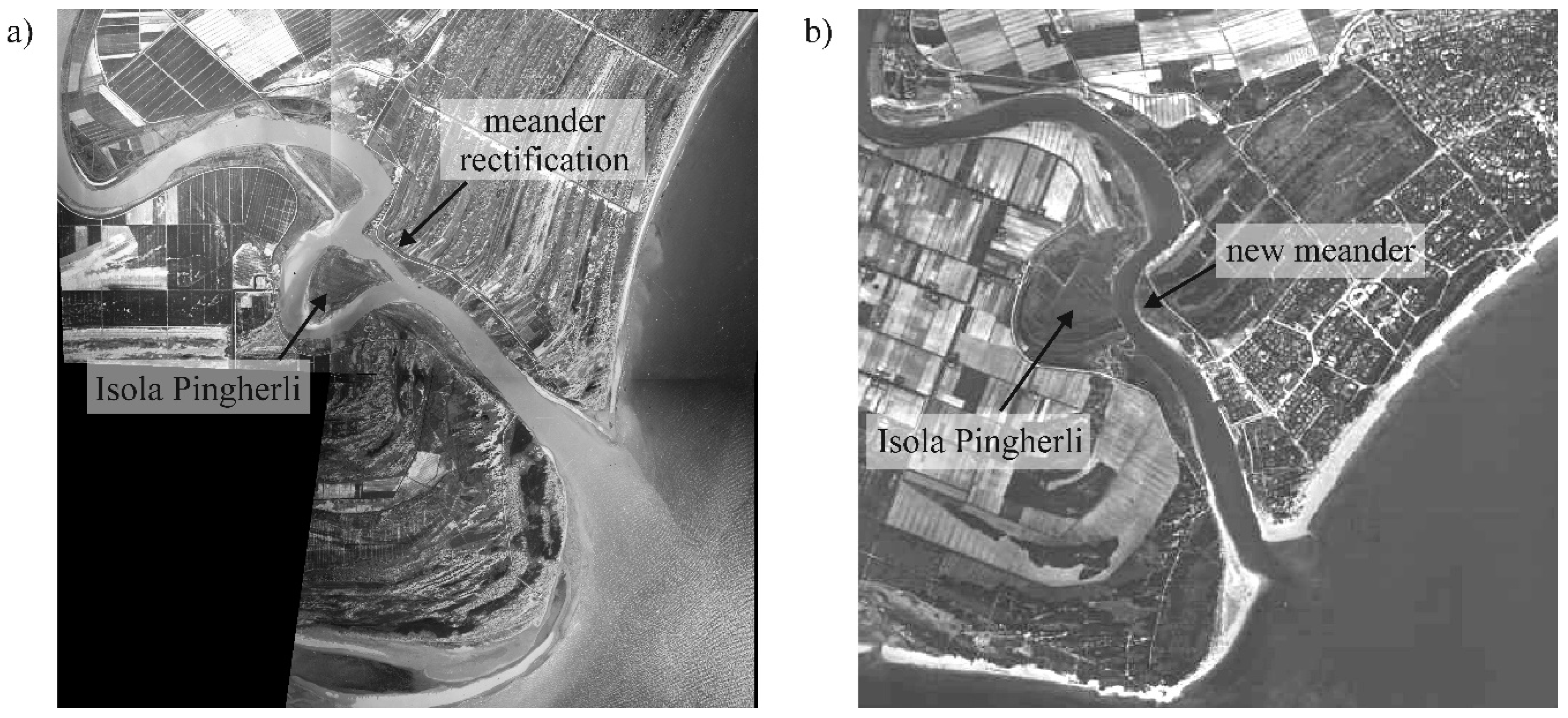
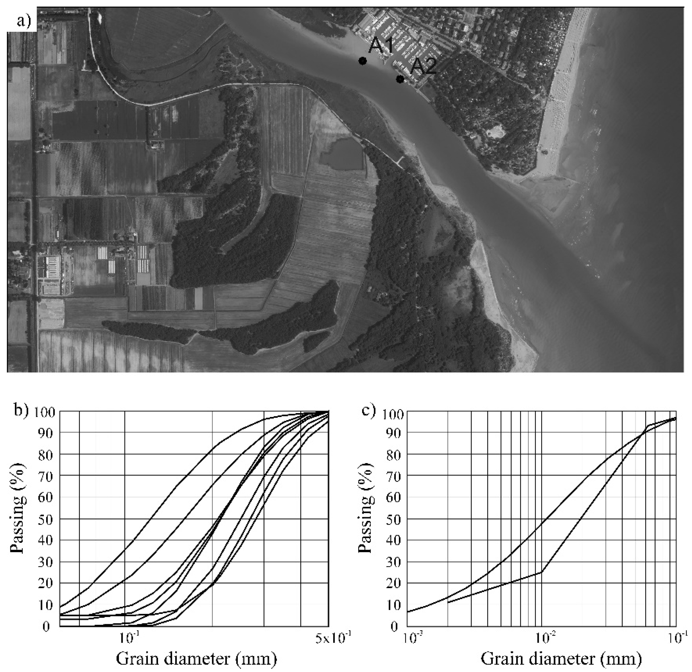
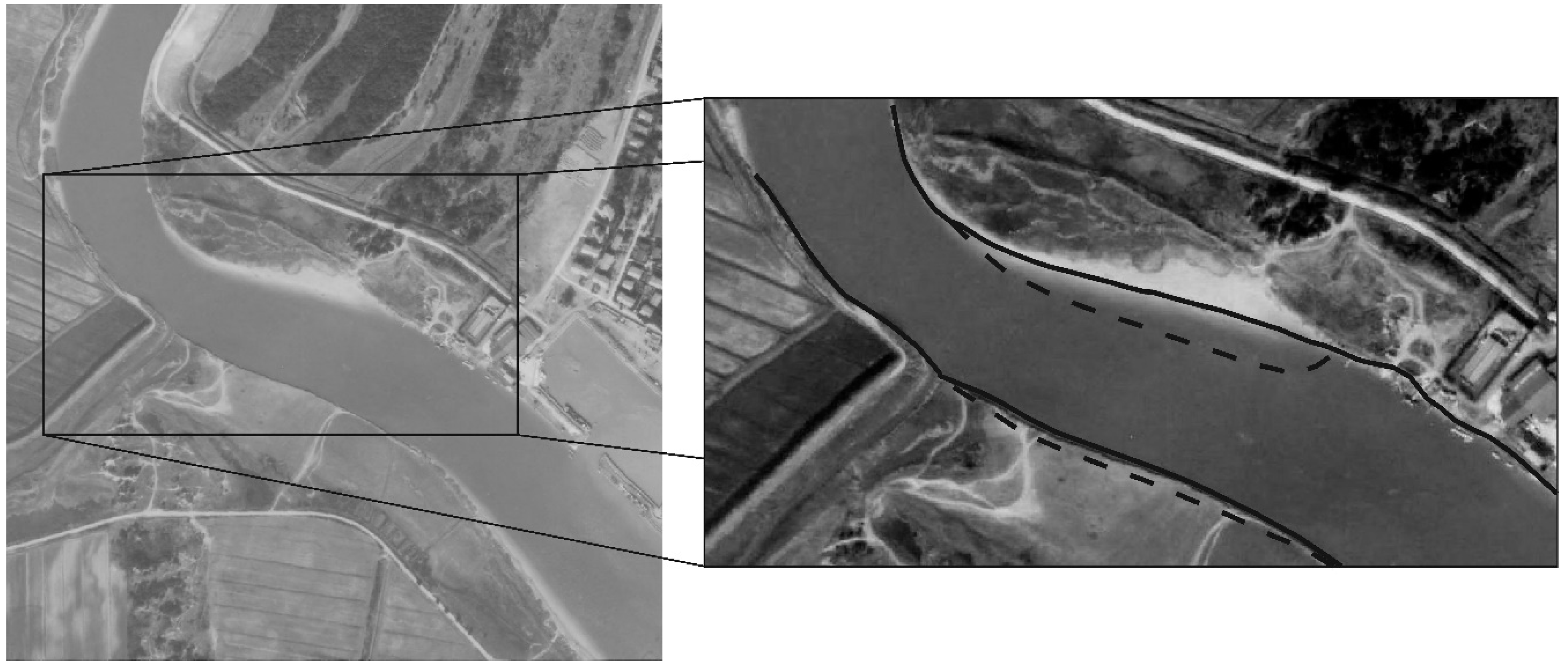
26]. This is the case of the Isola Pingherli site in the Tagliamento River (
Figure 4a). For this site, it was possible to acquire a set of historical aerial photographs, which are considered as one of the possible methods to identify channel migration [
69]. The main engineering work in this area was probably a meander rectification carried out in the late 1920s and which became the main stream of the river about 30 years later (
Figure 4a).
After a few years, the old meander deactivated, and the channel planform began to change, forming a new bend towards the river mouth, which began to become visible in the 1980s (
Figure 4b). In the present configuration, the river bend is still deforming itself, with a significant bank retreat on the right-hand side and accretion on the left-hand side. This area is one of the few in the lower course of the river, where a significant morphological evolution is occurring, because it is not constrained between fixed embankments.
Due to the availability of historical aerial photographs and a survey, taken in different reference years, this channel evolution represents an appropriate benchmark test case to apply a numerical model to investigate the capability of reproducing the bankline shifting over a mid-length period of some years. In particular, the years between 1983 and 1988 have been simulated (
Figure 5).
3.1. Field Site
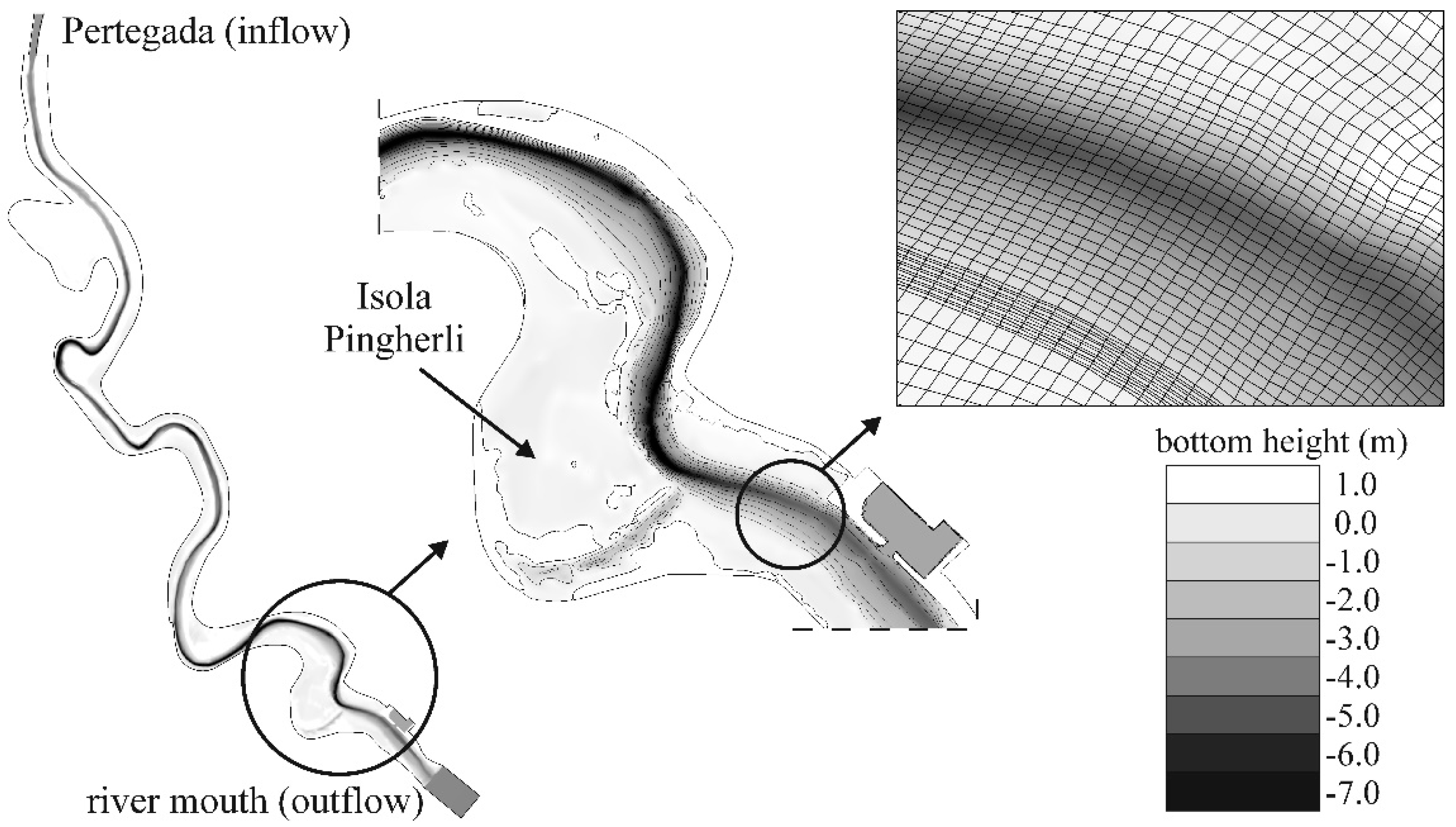
The modelled area includes the river and its banks, from the upstream section of Pertegada, to the river mouth, for a length of about 12 km. Cell size ranges from 2 to 3300 m2, where the smallest have been used to perform a better description of the bank slopes.
The beginning of the simulation has been set in 1983, at that time a detailed survey of the whole Tagliamento River was conducted by Barigazzi between 1982 and 1983, who measured about 30 cross sections in the field site, with a mean distance of about 500 m from one another [
70]. This was the last complete and detailed survey of the submerged bed of the river conducted.
The bottom height of the cells of the channel has been taken from the Barigazzi survey data, performing a linear interpolation between consecutive cross sections, while, for the height of the floodplains, it has been necessary to complete the Barigazzi survey data with recent laser surveys. In
Figure 6, the modelled area is depicted, together with a detail of the meander which is the object of this study and the computational grid used in the present simulation. This has been designed to represent the main channel as well as possible, following the flow direction and the river banks, which have been discretized with very tight cells. It can appear slightly coarse in some areas, especially in the flood plains behind the banks. Nevertheless, the adopted bank failure criterion, allows the bottom height to be lowered step-by-step; in this way, the bankline recession is clearly visible, when it exceeds the cell size. Hence, this procedure can be applied both with large and small cell sizes.
Barigazzi survey data, aerial photographs and a number of on-site inspections have been used to subdivide the mesh into three roughness classes representing the channel and low and high vegetated flood plains. The Manning coefficients assigned to each class are summarized in
Table 1 and have been deduced from a previous calibration process, conducted over a longer part of the Tagliamento River, from the Alps to the river mouth [
3], and in-line with the values proposed in literature [
71].
The boundary conditions adopted were inflow at the upstream section of Pertegada, tide at the river mouth and wall at the main embankments, even if preliminary simulations showed that the lateral side of the mesh has never been reached by the water.
3.2. Hydrometric Data
In the literature, the debate is still open on which kind of events are more influential on the morphological evolution of rivers: the small and frequent ones or the large and rare ones [
26]. In this respect, it should be underlined that, in the case of the Tagliamento River, the bank shifting observed over the last 30–40 years has not occurred in conjunction with extreme events, the last flood with a return time of about 100 years being registered in 1966. Following these considerations, it has been decided to represent the effects of a typical year, whose repetition is considered to be responsible for the bank processes.
Moreover, it is clear in the literature that bank erosion is not a continuous phenomenon, but it takes place occasionally, during flood events while the low flow period does not play an important role in this regard [
32]. To define the inflow boundary condition representing an average year, the hydrometric data recorded in the stations of Madrisio and Volta di Latisana in the period 2000–2012 have been analysed. Volta di Latisana is located approximately 3 km upstream of Pertegada and it is the closest recording station to the inflow section; nevertheless, its measurements are not always continuous in time and they are affected by tidal oscillations. Thus, the station of Madrisio, 24 km further upstream of Volta di Latisana, has also been considered, which is distant enough from the river mouth not to feel the influence of tides.
To convert water levels into flow rate, a stage–discharge relationship has been applied, which has been numerically deduced for the two measuring stations in previous work, considering flood propagation from the Alps to the river mouth and also including the effect of the Cavrato floodway, located between Madrisio and Volta di Latisana [
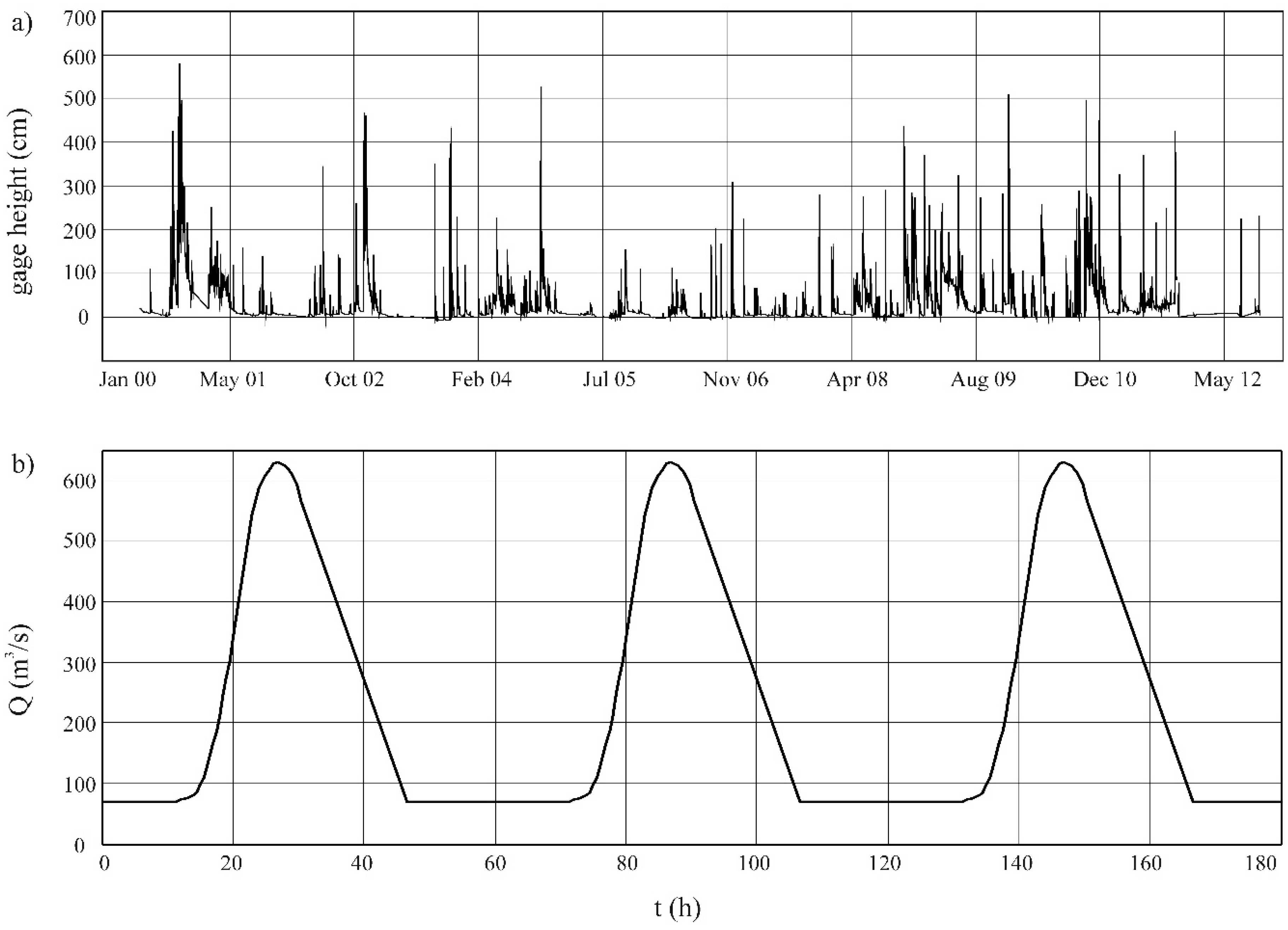
3]. Hydrological data depicted in
Figure 7a show that in the Tagliamento River there are on average three significant flood events in one year that exceed the gauge height of 2.70 m. Preliminary tests performed with the model show that only the events that exceed this threshold generate appreciable sediment transport. Using a simple statistical analysis on the events that exceed this threshold, a mean peak discharge of about 630 m
3/s in Volta di Latisana has been evaluated. Moreover, the form of the registered flood events has been analysed and an average shape has been obtained. Thus, as the inflow boundary condition, an equivalent hydrograph has been adopted with three reconstructed medium flood waves, having form and peak deduced from registered data (
Figure 7b). The influence on the river evolution of low flow periods between two flood episodes is very limited, thus in this work the flood waves are spaced by 25-h steady flow, with a discharge of 70 m
3/s, which is the average annual flow rate. The 25-h intervals have been chosen to assure the deposition of the sediments entrained by the current during each event.
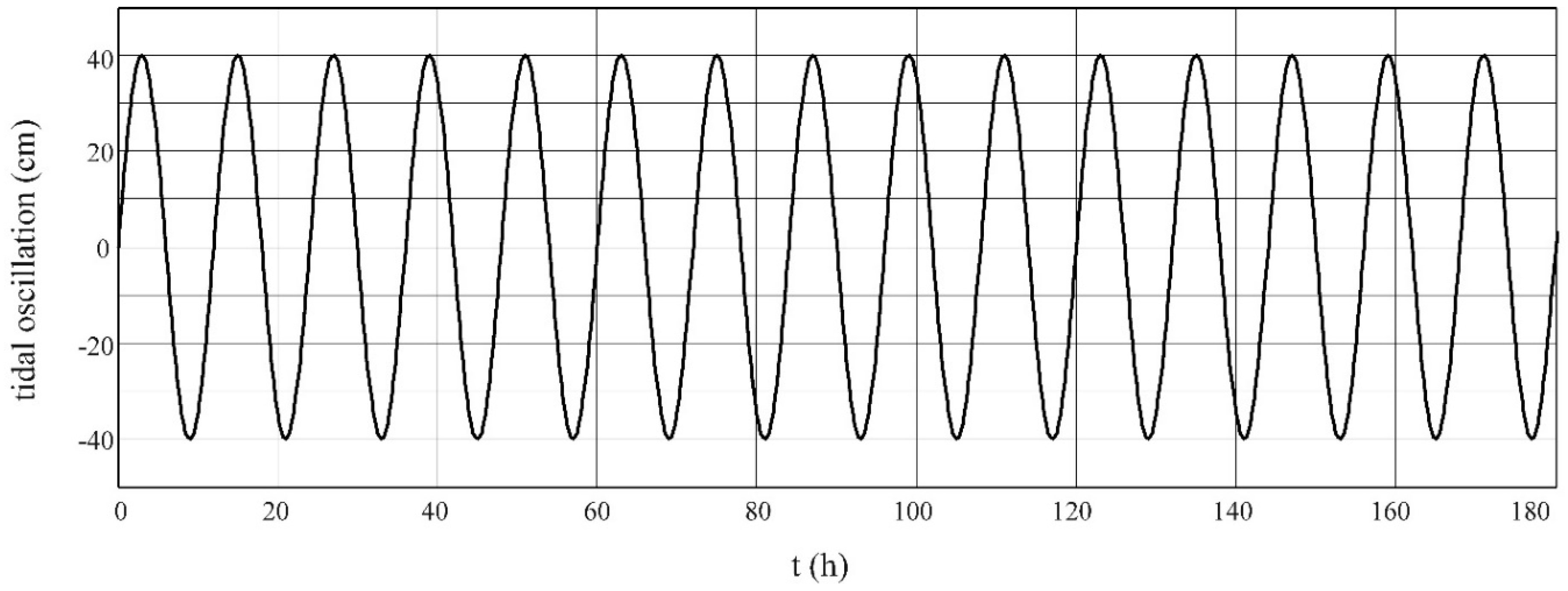
As the tidal boundary condition, a sinusoidal oscillation has been imposed, with a period of 12 h and amplitude of 40 cm, which are the mean values obtained from the analysis of the tidal hydrometric data recorded in the studied area in the period 1991–2014 (
Figure 8). Flood wave and tidal oscillation have been combined as depicted in
Figure 7 and
Figure 8, after evaluating with preliminary analysis that a phase shift of the peak flow with respect to the tide does not lead to substantial variations in the results.
3.3. Sediment Data
The assumption about sediment data has been deduced from measurements performed over the last few years, which highlight the presence of both granular and cohesive sediments, having a mean diameter of 210 μm and 18 μm, respectively (
Figure 9). Moreover, the mean grain density is 2760 kg/m
3 and the porosity is assumed as 0.35. The cohesive layer extends on average down to 3 m under sea level.
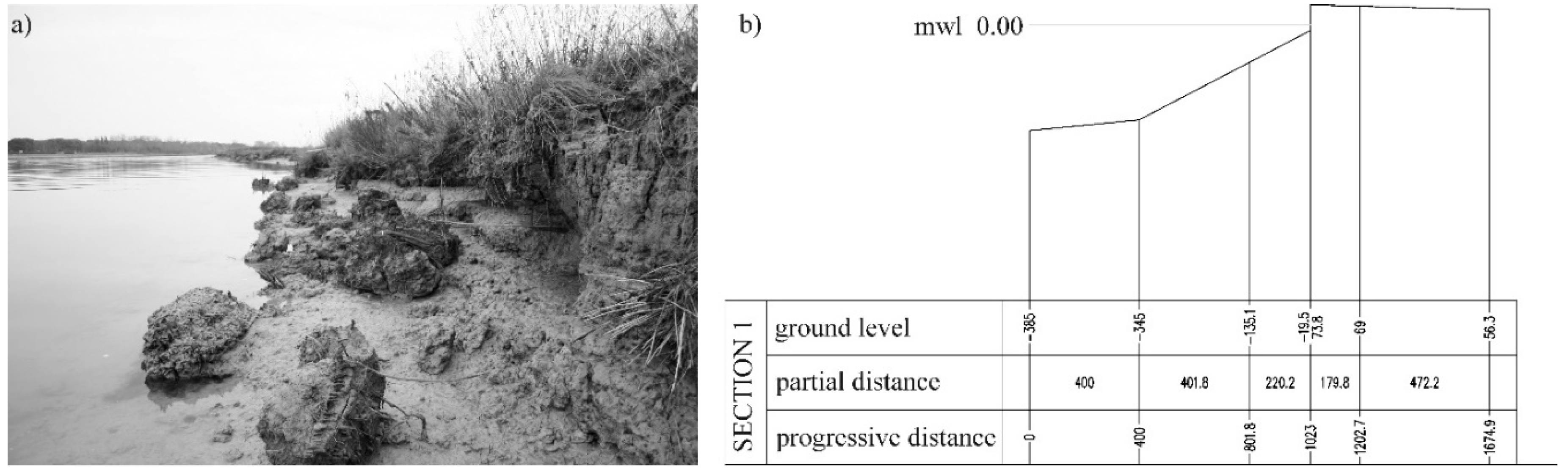
As already stated, in the literature, different bank failure mechanisms have been presented and their choice can be justified through direct observation [
26]. In the Tagliamento River case, the right-hand side bank is formed by an upper, almost vertical side with a lower and less steep slope (
Figure 10). Moreover, after an ordinary flood event, some blocks of material, failed from the banks and not yet removed by the flow, are clearly visible. This situation can be considered as representative of the erosion mechanism in this area, regardless of the year they refer to. Both figures indicate that the upper part of the bankside keep a vertical profile until the stream erodes it; the small compact masses of sediments, that can be seen in the pictures, suggest a sequence of discrete local slumps of bank material, probably due to a cantilever failure, triggered by the lateral erosion process. These blocks will be taken away by the next flood event. The lower part of the bank slope is usually submerged and it shows a lesser steepness, probably caused by the reduction of the soil shear strength compared to the emerged part due to swelling and shrinkage, as highlighted, for example, by Spinewine et al. [
64]. The local failure operator introduced in the developed model seems to be appropriate to describe the observed phenomena.
Furthermore,
Figure 10a shows that bed and lateral roughness are very similar and this fact corroborates the decision to adopt the same shear stress to the bottom and to the side wall.
In the literature, a great variability of the values for the critical erosion bed shear stress
τe is observed, with values covering more than two orders of magnitude [
26,
29,
41,
42]. In the present paper, a mean value of 1 Pa for
τe has been adopted, which is within the range of both the Thorn and Parson and Mitchener formulae [
43] and also in line with the values experimentally obtained by Amos et al. [
44] for saltmarshes in the nearby Venice lagoon. Moreover, a sensitivity analysis has been conducted to check the influence of this parameter in the overall result. For the critical bed shear stress for deposition, a value of 0.06 Pa has been assumed.
Regarding the angle of repose of submerged material, in the literature, different values have been proposed and the choice among them is still ambiguous [
33]. In the present paper, a value of 35° has been adopted for the residual angle, after the avalanching process occurred, as an average deducted from the recent survey of the bank (
Figure 10b). Thus, the angle of initial yield has been assumed a little higher (
φi = 40°).
Concerning the sediment boundary conditions, it is not easy to evaluate the suspended load entering the domain, because transport is often supply-limited [
26]; nevertheless, in the present work, an equilibrium formula has been adopted for the granular material. With respect to the cohesive suspended load, this has been calibrated to be in equilibrium with the upstream part of the computational grid. Moreover, the inflow of sediments seems not to have an important role in the bank migration process; in fact, the boundary conditions have been set far upstream from the field site, to let the model adjust itself.
3.4. Model Results and Discussion
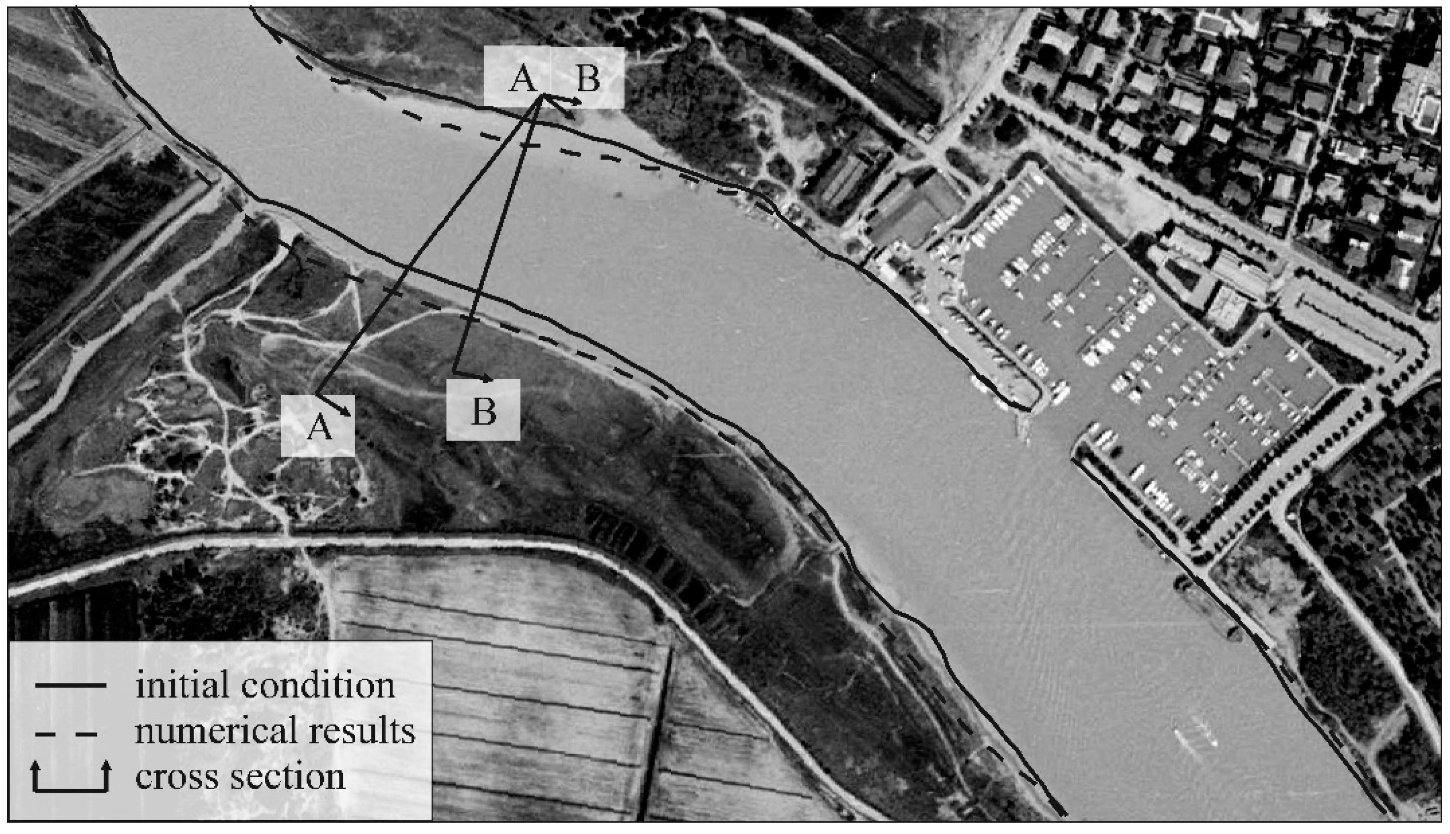
To check the ability of the model to describe the phenomenon, a simulation has been conducted to reproduce the morphological evolution which occurred over a five-year period. The numerical results are compared with the first available aerial photograph after the Barigazzi survey, i.e., an image taken in 1988. In
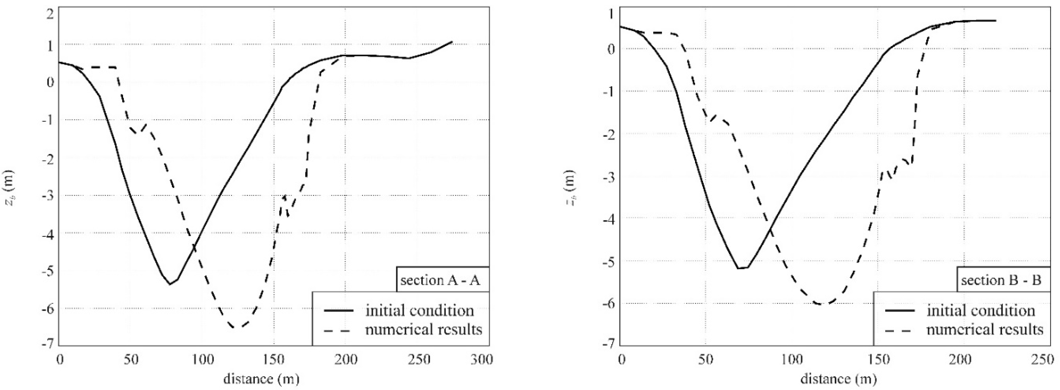
Figure 11, the outcomes in terms of shoreline migration are shown: the continuous and dotted lines represent the 0 m height at the beginning and end of the simulation, respectively. The numerical result shows a trend of movement of the meander towards the river mouth, with a displacement of the channel to its right. Land accretion is observed, associated with sediment deposition at the inner bank; on the contrary, at the outer side of the meander, a bank retreat is noticed. The comparison between the numerical results and the aerial image points out overall good agreement, with a small deviation in particular upstream and downstream for the part of the outer bank. In particular, the left-hand side bank reveals a maximum accretion of about 20 m, both in the numerical and experimental data. The simulation shows a retreat of the right-hand side bank of about 25 m in the most exposed part, which decreases moving downstream to about 9 m at the meander apex; the comparison of 1983 and 1988 data in the same area shows an almost constant recession of about 10–11 m. Moreover, the cross sections depicted in
Figure 12 highlight a deepening of the river, associated with displacement.
Furthermore, it is worthwhile underlining that, in all the performed simulations, the channel width has not varied substantially. In 1983, its mean value stood at about 137 m in the survey and at about 132 m in the 1988 image; at the end of the five-year simulation, the channel width was about 140 m. Thus, the channel width seems not to change, confirming a migration of the river cross section, with no major deformation. This fact suggests that the present width is an equilibrium one for the flow regime of the Tagliamento River and that its planform evolution does represent a morphological response to the meander rectification carried out in the late 1920s.
The description of the shoreline retreat on the right-hand side of the river has been made possible by the failure criterion, which considers the effects of the flow-induced lateral erosion. Bank failure with cohesive sediment materials is a very complex geotechnical process with a strong stochastic component [
25], which would need a dedicated geotechnical model to describe the apparently random and sudden cohesive bank material collapse shown in
Figure 10a. The present scheme does not seek to represent the instant phenomenon; instead, it considers only the total cohesive mass removed from the bank within one year or more, by both erosion and consequent instability. The resulting scheme turns out to be very simple, with few parameters to be calibrated. This is consistent with the simplifications introduced in the hydrodynamic model, which is developed within the framework of shallow water theory. The shallow water equations are an approximation of the tridimensional equations and, in this way, they are not able to describe all complex tridimensional phenomena; the failure criterion follows the same philosophy. Nevertheless, the results show that this simple scheme describes the bottom and planimetric evolution of the river in a proper way.
A sensitivity analysis has been conducted to check the influence of the critical erosion bed shear stress
τe on the results, concerning the morphological evolution of the meander. Two further simulations have been carried out, having
τe equal to 0.7 Pa and 1.2 Pa, respectively. The results are depicted in
Figure 13 as the shoreline at the end of the process. As expected, there is no effect in the accretion of the inner side of the meander, where the three curves are superposed. Conversely, the impact of this parameter is more evident in the outer side of the meander, where the bankline retreat increases with decreasing values of
τe. Moreover, it can be noticed that the deviation of the outcomes adopting 1.2 Pa instead of 1.0 Pa is limited and both give rise to results that are in good agreement with the observed bank shifting. Instead, the diversion grows significantly when using the lowest value, and the numerical and observed bank recession drift apart.
4. Conclusions
This paper describes a 2DH morphodynamic numerical model, suitable to simulate the medium-term evolution of a river in its lower course, where there may be both granular and cohesive sediments. The model combines bidimensional shallow water equations with two transport equations, the former for granular and the latter for cohesive sediments concentration. The bed level change is evaluated through a sediment continuity equation on a control volume near the bottom.
The work focuses on the capability of the model to describe both bed deformation and bankline shifting in 2D planform. To this aim, a failure criterion was included in the numerical scheme, which evaluates at every time step and, with a specially developed method, the lateral erosion due to the flow and the consequent cantilever collapse. One advantage of the proposed technique is that the lateral erosion and the consequent cantilever failure are considered together as a whole, being two parts of the same process, which causes the shift of the bank. The model works with quadrangular irregular fixed grids; thus, the lateral erosion cannot be reproduced moving the cell edge representing the toe or the top of the bank, but it is simulated removing the eroded material from the cell at the top of the bank and relocating it at the toe of the bank, raising the bottom height of the corresponding cell. The reduction of the bottom height of the cell representing the top of the bank also allowed flood waves and high tides to occupy areas which would otherwise have remained dry and hence which would not be involved in sediment transport processes. It is worthwhile underlining that this procedure does not need the user to select whether a cell belongs to the bank, because the vertical slope of the bank is automatically recognized when a wet–dry front is encountered, with the bottom height of the dry cell being higher than the water surface of the wet one. In addition, the mesh does not need to be reshaped during the simulation.
Moreover, geostatic instability due to submergence is considered by means of an avalanching mechanism. The model was applied on the final reach of the Tagliamento River in northern Italy, which is undergoing a strong evolution process due to the migration of a meander which was triggered by a rectification carried out in the last century. The sediment properties as well as the failure criterion were deducted from measurement campaigns and photographs. Hydrological forcing responsible for a one-year morphological evolution was assumed and a five-year simulation was carried out. Numerical results show that the model can adequately describe the general morphological evolution of the meander. The inner bank accretion was well represented and the outer bank recession was also predicted. Finally, a sensitivity analysis on the critical bed shear stress for cohesive sediments was conducted, which showed that a small increase of this parameter does not lead to a meaningful variation of the results; however, a reduction causes a large deviation of the results.


