Article

Sensitivity of Soil Moisture Analyses to Contrasting Background and Observation Error Scenarios

by
Joaquín Muñoz-Sabater
1,*,
Patricia De Rosnay
1,
Clément Albergel
2 and
Lars Isaksen
1
1
European Centre for Medium Range Weather Forecasts, Shinfield Road, Reading RG2 9AX, UK
2
CNRM UMR 3589, Météo-France/CNRS, 31057 Toulouse, France
*
Author to whom correspondence should be addressed.
Water 2018, 10(7), 890; https://doi.org/10.3390/w10070890
Submission received: 9 April 2018 / Revised: 15 June 2018 / Accepted: 22 June 2018 / Published: 4 July 2018
(This article belongs to the Special Issue Monitoring and Predicting Soil Moisture and Drought Conditions)

Abstract

:
Soil moisture is a crucial variable for numerical weather prediction. Accurate, global initialization of soil moisture is obtained through data assimilation systems. However, analyses depend largely on the way observation and background errors are defined. In this study, a wide range of short experiments with contrasted specifications of the observation error and soil moisture background were conducted. As observations, screen-level variables and brightness temperatures from the Soil Moisture and Ocean Salinity (SMOS) mission were used. The region of interest is North America, given the good availability of in situ observations and mixture of different climates, making it a good test for global applications. The impact of these experiments on soil moisture and the atmospheric layer near the surface were evaluated. The results highlighted the importance of assimilating observations sensitive to soil moisture for air temperature and humidity forecasts. The benefits on predicting the soil water content were more noticeable with increasing the SMOS observation error, and with the introduction of soil texture dependency in the soil moisture background error.

1. Introduction

Soil moisture is a very important variable for short and medium range weather predictions. The reason is the strong influence that it has on the partitioning between latent and sensible heat fluxes at the soil–atmosphere interface, and therefore on the boundary layer development [1,2]. Small changes in the initialization of the soil moisture field can produce significant model drifts at different temporal scales [3,4,5,6], so it is of crucial importance to accurately estimate soil moisture for Numerical Weather Prediction (NWP) systems.
The last decade has seen a large number of studies using data assimilation methods to constrain soil moisture with available in situ and remotely sensed observations [7,8,9,10]. An important component of these systems is their ability to incorporate not only the information from independent observations, but also its associated uncertainty. By assigning accurate weights to observations and the model background, data assimilation systems are able to produce an optimal (or suboptimal) estimate of the soil moisture state, which is generally of superior quality to that of only model based estimates. It is difficult to assign accurate errors to a blend of observations and model estimates which represent all the known sources of uncertainties (instrumental errors, simplifications of the algorithms, errors in model parameterisation, inaccurate atmospheric forcing, and representativeness errors). This is not a straightforward task and indeed there is very little knowledge of the correct specification of these errors in soil moisture related data assimilation systems. A diverse range of approaches can be found in the literature. In [11], the dispersion of in situ surface soil moisture observations is used to specify the input errors of the observation error covariance matrix in several assimilation schemes, however this estimate did not account for the spatial representativeness error. Other studies used empirical values based on field experience or ensemble methods. For example, Munoz-Sabater et al. [12] used an ensemble of model integrations to produce an estimate of the background error. A more physically-based relationship between relevant land parameters was tried by Mahfouf et al. [13] to obtain representative errors of soil moisture. They specified the diagonal terms of the soil moisture background error covariance matrix as a function of the water holding capacity (field capacity minus wilting point), thus related to soil texture. More recently, the triple collocation technique has become popular for generating spatially explicit error estimates of soil moisture data [14,15]. Although these methods do not guarantee the correct weight given to observations and model fields, they can be considered as a necessary calibration step towards optimal use of the information content of the background and observations in a data assimilation system.
In this paper, different configurations for the observation and background error covariance matrices in the European Centre for Medium-Range Weather Forecasts (ECMWF) Simplified Extended Kalman Filter (SEKF) soil moisture analysis were evaluated. The SEKF [16,17] was used to analyse soil moisture of the top three layers of the H-TESSEL land surface forecast model [18] used in the Integrated Forecasting System (IFS) at ECMWF. The soil moisture background value is adjusted by assimilating 2 m temperature and 2 m relative humidity observations (as proxies for soil moisture), and brightness temperatures ( T B ) [19] observations from the Soil Moisture and Ocean Salinity (SMOS) mission of the European Space Agency (ESA). Currently, the background error information used in the operational SEKF is static, in both time and space. Likewise, screen level observation errors are also constant, whereas, for SMOS observations, the pure radiometric accuracy, specific to each observation and with typical values within 2.5–3 K (as specified in Section 3 of [10]), has been used as an estimate of the observation error. The main goal of this study was to investigate the sensitivity of soil moisture analyses to different background error and SMOS T B error specifications in the SEKF and thus provide useful recommendations for a configuration suitable for operational implementation at ECMWF. A range of data assimilation experiments were conducted, using different approaches (SEKF or pseudo-direct insertion, as explained in Section 2.3), with SMOS data combined or not with other types of observations. Different configurations of the SMOS observation error (increasing or decreasing the confidence in the observations) and model background error representation (static or propagated in time, with or without soil texture dependence) were investigated. Results of these experiments were compared against in situ data from the USCRN and SCAN networks in US. In addition, the sensitivity of the near-surface layer in the atmospheric model was also evaluated.

2. Methodology

2.1. The ECMWF Soil Moisture Analysis

The ECMWF soil moisture analysis is a point-wise SEKF that uses an assimilation window of 12 h to be compatible with the assimilation window of the upper-air analysis. It is based on the minimization of a cost function J as in a variational approach:
J ( sm ) = ( sm sm b ) T B 1 ( sm sm b ) + ( y o H ( sm ) ) T R 1 ( y o H ( sm ) )
where sm is the state vector consisting of the soil moisture of the top three layers of the ECMWF land surface model H-TESSEL, sm b is the background state, yo is the observation vector, H is the non-linear observation operator projecting the model background into observation space, B is the error covariance matrix associated with the background soil moisture state and R is the observation error covariance matrix. The diagonal elements of B and R represent the variance of the background error and of the observation error, respectively. The off-diagonal terms represent cross-covariances. In the operational version of the SEKF, the error matrices are assumed to be diagonal.
The SEKF combines screen level observations (2 m temperature and 2 m relative humidity) and satellite observations (currently there are capabilities implemented to assimilate Advanced SCATerometer [ASCAT] soil moisture retrievals and SMOS T B observations) with model estimates to adjust the soil moisture background state. The analysis equation at time t i is defined as [20]:
sm a ( t i ) = sm b ( t i ) + K i [ y o ( t i ) H i ( sm b ) ]
with superscripts a, b, and o standing for analysis, background and observations, respectively. The Kalman gain matrix K i , computed at time t i , is defined as:
K i = [ B 1 + H i T R 1 H i ] 1 H i T R 1
with H i the linerised version of the observation operator that is numerically computed by finite differences. In a Kalman Filter, the background error covariance matrix evolves between time i and i + 1 according to the law of propagation of uncertainties as:
B i + 1 = M B i M T + Q
where M is the linearised prognostic model operator, and Q is the model error covariance matrix. Integrating this equation for large dimensional problems is computationally very demanding, but affordable for low-dimensional point-wise analysis problems as in this study. It is important to notice that the Kalman Gain depends on B and R at the time of the computation, as in this study various formulations for B and R are investigated.

2.2. Errors Specification

In the current operational configuration of the ECMWF SEKF, it is assumed that the background error covariance of the state variables is constant during the whole assimilation period, and with a value equal to 0.01 m 3 m 3 for each model grid point and soil layer. This approach is rather simplistic and conservative, and assumes that the model soil moisture of the top three layers is affected by the same errors. However, the top layer is subject to larger variability, especially after rain events, making larger background errors more likely to happen than in the relatively more stable deeper layers. Another very important parameter for soil moisture modelling is soil texture. Soil texture is obtained from the Food and Agriculture Organization (FAO) data set, whereas sand and clay fractions have been computed from a lookup table according to [21]. Soil moisture variability with depth and soil texture are two crucial factors in soil moisture modelling, and are not accounted for in the current definition of background errors. In this study, these two factors were considered to set up different scenarios for the background error, as described in Section 2.3. The standard deviation of the screen-level temperature and relative humidity observations error are constant and set to 1 K and 4%, respectively, as in the operational SEKF configuration at ECMWF. Each multi-angular, multi-polarised SMOS T B observation is assigned an error equivalent to its specific radiometric accuracy. This is an objective measurement of the error associated to each observation. However, this approach likely gives unrealistically high weight to the SMOS observations in the assimilation system, as it does not account for other sources of instrumental errors and of horizontal and vertical representativeness errors of the measurement. Note that, following the approach adopted in [17] and [10], the correlation between SMOS T B observations at different incidence angles is neglected in this paper. This issue is not within the objectives of this paper and it requires a dedicated study. The use of ensemble methodologies implicitly resolves this problem, although additional assumptions are needed [22,23]. Based on the above shortcomings in the specification of model and observation errors, in this study different error scenarios are tested, as described in the next section.

2.3. Experiment Types

A series of one-month assimilation experiments at approximately 40 km horizontal spatial resolution (equivalent to TL511 triangular spectral resolution with linear grid) were run over North America. Their aim is to test the impact of different observation error and model error scenarios on soil moisture and the near-surface atmosphere in this region. The period of integration spans from 15 September 2012 to 14 October 2012. This is a period of hydrological recharge in the US, and therefore with strong variability of soil moisture and suitable for the objectives of this study. In these experiments, SMOS observations were assimilated at incidence angles of 30°, 40° and 50° with a margin of one degree around these angles to get a sufficient number of observations. Further, all the observations in each angular bin were averaged to reduce the observational noise [24]. Only the pure XX and YY polarisations (which is equivalent to the H and V polarisations, but in the satellite antenna reference frame [see, for example, [25]) were used. Only the Alias Free Field-Of-View (FOV) was considered, as being the area of the FOV delivering data of highest quality. SMOS flags from the Near Real Time (NRT) product were used to filter data affected by Radio Frequency Interference (RFI). Although these flags are useful to remove contaminated observations, one should bear in mind that they cannot guarantee to remove all observations affected by RFI. Further quality checks applied within the ECMWF SEKF can reject observations that were not detected by these flags (see, for instance, Figure 5b of [10]). All SMOS observations were bias corrected by accounting for the climatological differences (mean and standard deviation) between SMOS T B observations and the model equivalents obtained with a low frequency passive microwave radiative transfer model. To obtain rescaling coefficients accounting for the seasonal meteorology, a seasonal linear rescaling approach was conducted following the same approach as in [26]. More information about the bias correction scheme applied to SMOS data will be published later in [27]. The physical parameterisations of ECMWF model version cy40r1 were used in these experiments and the full coupled land-atmosphere system was employed. The upper-air atmospheric analysis was based on the 12-h 4DVAR system. However, to reduce the computational cost of these experiments, only in situ observations and satellite data from the Advanced Television and Infrared Observational Satellite (ATOVS), Ground Based Radar precipitation data (GBRAD) and Next-Generation Radar (NEXRAD) were used to constrain the atmospheric integrations. The consequence of using such a reduced observational system is the loss of accuracy in the spatial-temporal evolution of the atmospheric variables, whereas it is assumed that the impact on surface variables is small for the area and period under study.
The following experiments were defined:
(i)
OL: Open-loop configuration where the soil moisture state evolves freely in the 12 h land assimilation window without any additional observational constraint, i.e., no soil moisture analysis is performed.
(ii)
SLV: Screen-level variables assimilation only, which updates the soil moisture state based on indirect information provided by in situ observations of 2 m temperature and 2 m relative humidity.
(iii)
SMOS: SMOS T B assimilation only, with the model background error static during the whole assimilation cycle.
(iv)
SLV+SMOS: Combined assimilation of screen-level variables and SMOS T B with observation errors and background errors as defined in Section 2.2.
(v)
SMOS+Bprop: SMOS T B assimilation only, but enabling the propagation of the background error according to the SEKF equations. In this experiment, the model error was set to 0.01 m 3 m 3 at the start of the assimilation window for each model layer.
(vi)
SMOS+PI: In this case, the soil moisture analyses were substituted by the observed SMOS T B projected into control space. Thus, the soil moisture analysis is obtained by inverting the observation operator applied to the observed T B . This approach gives maximum weight to the observations. The term PI (pseudo-insertion) refers to the fact that SMOS observations are still subjected to the different quality controls applied in the ECMWF SEKF, so at each time the observation was rejected the analysed soil moisture value is equal to its background value.
(vii)
SMOS+2R: SMOS T B assimilation only, but the default error assigned to each observation was doubled, and therefore decreasing the influence of the observations.
(viii)
SMOS+Btext: SMOS T B assimilation only, but the background error was a function of the water holding capacity (WHC), defined as the difference between the soil capacity and the wilting point. Given that the land model used in this study used a global map of soil texture types, each of them with its own saturation and wilting point, the error in this experiment is a function of the soil texture type, and it will be larger for those soils with larger holding capacity, as organic type. An error of 10% of the WHC was assumed which for a medium soil texture type is equivalent to 20 mm of error integrated over the first metre of soil.
(ix)
SMOS+3DB: SMOS T B assimilation only, but assuming a background model error that depends on both the horizontal and the vertical dimension (3DB). In this case, it is assumed that the short term variability and precipitation errors affect mainly the top layer, whereas the root-zone is less affected. An error of 20% of the WHC was set for the top layer, whereas this error was halved for the second soil layer (7–28 cm), and it was assumed to be only 5% of the WHC for the third layer (28–100 cm).
The performance of these experiments was evaluated in terms of soil moisture analyses and the impact on the near-surface atmosphere. Three different groups were defined with the aim of studying several aspects of the type of assimilated data and the observation uncertainties or model uncertainties used in the SEKF:
  • Group I (OL, SLV, SMOS and SLV+SMOS): This first group of experiments was created to study the impact of the different type of observation assimilated in the SEKF. In this group, the OL experiment was used as the control experiment.
  • Group II (SMOS+PI, SMOS, and SMOS+2R): This second group of experiments was intended to investigate the effect of giving different weights to SMOS T B when only this type of observation was assimilated. The SMOS experiment was used as control in this group.
  • Group III (SMOS, SMOS+Bprop, SMOS+Btext, and SMOS+3DB): In this group, the influence of different definitions of the background error covariance matrix in the analyses of soil moisture was investigated. Experiment SMOS was used as control as well.
In addition, all the previous experiments were also compared in a unique group. Table 1 recapitulates the main assimilation aspects of these experiments. Note that the short period of analysis and the reduced atmospheric observing system used in the above experiments were necessary to afford to undertake all the proposed experiments. The likely consequence is a loss on the statistical significance of the results, however it is expected that even at these short time scales useful features can be observed.

2.4. Evaluation and Verification Strategy

The evaluation of each of these experiments’ soil moisture analyses was conducted by comparison against in situ data from the U.S. Climate Reference Network (USCRN) and the Soil Climate Analysis Network (SCAN) in the US. The location of these stations can be observed in Figure 1. For the SCAN network, a total of 177 stations were used in this study. This network (http://www.wcc.nrcs.usda.gov/scan/) spans all over US, and provides comprehensive information of soil moisture and climate, designed to support natural resource assessments and conservation activities with a focus on agricultural areas in the United States. Long data records of soil temperature, soil moisture at several depths, soil water level, air temperature, relative humidity, solar radiation, wind, precipitation, and barometric pressure, among others, are available for this network. The vegetation cover at those sites consists of either natural fallow or short grass. The second network used to evaluate soil moisture analyses is the USCRN from the Oceanic and Atmospheric Administration’s National Climatic Data Center (USCRN NOAA’s NCDC), consisting of 114 stations developed, deployed, managed, and maintained by NOAA. This network was built with the purpose of detecting the national signal of climate change. For both networks, soil moisture data are available at hourly time steps and were collected at five standards depths; 5, 10, 20, 50, and 100 cm.
In this study, both the top model layer and the root-zone layer analyses were evaluated. For the top layer, the average of the 00, 06, 12 and 18 UTC daily analyses, representative of the first 7 cm of soil, were compared to the daily four equivalent in situ observations located at a depth of 5 cm. For the root-zone, the observations up to 1 m depth were used to build a weighted average proxy of root-zone soil moisture. The measurements of all these probes at the previous synoptic times were averaged daily and compared to the average of the equivalent daily 00, 06, 12 and 18 UTC analysis of the top three model layers, which are representative of the first metre of soil. Only ground stations with available measurements at 5, 10, 20, 50 and 100 cm were retained. Stations with gaps in the time series of in situ measurements under the period of study were discarded too. To filter out ground stations potentially affected by frozen conditions, a temperature of 4 C was used as threshold below which in situ measurements were not used. The same approach can be found in other studies, as in [28]. The bias, the unbiased root mean squared difference (ubRMSD) and the time-series correlation coefficient (R) of the analyses compared to in situ data were computed for each station and averaged per network over the length of the experiment. This choice of metrics provides information on different aspects of the analyses’ skill [29], in particular biases with in situ observations (assuming that the in situ soil moisture data represents the “truth”), the standard deviation of the differences and the relative temporal variability of soil moisture time series. The p-value test was used to exclude suspicious in situ data with non-significant R values, as in [30]. The correlation was considered not to be a coincidence if the p-value test was below 0.05.
The impact of these experiments on the near-surface layer of the atmospheric model was assessed by comparing the 2 m temperature and 2 m dew point temperature forecasts against observations from the SYNOP network. Figure 1 presents the region and the SYNOP observations that were retrieved and used for evaluation purposes. The impact of these experiments at short range forecasts and in the daily cycle were evaluated by using four synoptic forecast times: 12, 24, 36 and 48 h, respectively. A total of 30 forecasts were averaged for each synoptic time, based on forecasts started at 00 UTC. Finally, the forecast skill score of an experiment averaged over the whole region under study was computed for air temperature and air humidity near the surface and up to a maximum of 10 days. In this paper, the forecast skill score is defined as the difference in root mean squared (RMS) forecast error between the experiment and its control, normalized by the control RMS. The forecast error is defined as the difference between the forecast and the operational analyses. The operational analysis was taken as reference since it uses the full observing system, providing the best reference for evaluation [31]. This approach is commonly used at all NWP Centers, including ECMWF, to verify the forecasts and to assess the impact of new observations. A value of the forecast skill score was obtained by averaging the daily scores over the 30-days period.

3. Results

3.1. Soil Moisture Evaluation

Table 2, Table 3 and Table 4 show the evaluation of the Group I, II and III soil moisture analyses against all available observations from the USCRN and SCAN networks, respectively. These tables are split between the first model layer (where remote sensing observations show sensitivity) and the first metre of soil where the plant roots extract water from the soil. Note that for the SCAN network some ground stations (for the three groups of experiments) are clustered on the western US, which may slightly bias the averaged metrics towards this area.

3.1.1. Group I

In Table 2, the type of assimilated observation was investigated. For the USCRN network, 38 stations passed all the quality control for evaluation, whereas 58 did for the SCAN network. Assuming that the in situ soil moisture observations are bias free, the largest biases are obtained for the free soil moisture run configuration (OL) and the experiment assimilating only screen temperature and humidity observations (SLV). This occurred for both the top layer and the root-zone. Whilst this result might be expected for the free run as the model soil moisture is not constrained by any observations, one might expect a closer match to the in situ data with the screen-level constraint. However, we did not see any improvement compared to the free run. This result is in very good agreement with the study of Drusch and Viterbo [5], where the soil moisture analyses of an Optimal Interpolation (OI) scheme using screen variables were not superior to those forecast by an open loop. The case presented here differs mainly in the use of an advanced assimilation scheme, the SEKF [16,17], yet the results in terms of soil moisture analysis are very similar to the open loop. The SEKF was also used by [17] and they confirmed a slight improvement of soil moisture compared to an OI scheme. Apart from the fact that screen-level data do not provide a direct observation of soil moisture, the combination of several other reasons can support these neutral results: firstly because the approach used in the SEKF is very conservative, giving very little weight to screen observations and therefore producing very small increments; secondly because the assimilation period used in these experiments is short, which is not enough to observe the impact of the small screen data increments at longer time scales; and, finally, because, even if screen data have been spatialised in a previous step, there is a small number of SYNOP observations influencing the analyses close to the stations of these networks. Locally for some stations, some differences are observed (not shown). These results are consistent with other studies where the assimilation of screen observations had negative effects on soil moisture while improving surface fluxes [4,5]. Introducing SMOS observations in the observation vector, either alone or in combination with screen variables, reduced the biases on average over both the USCRN and SCAN network, and in particular for the experiment assimilating only SMOS T B . On the other hand, the experiments using SMOS T B increased the ubRMSD and degraded the correlation coefficient.
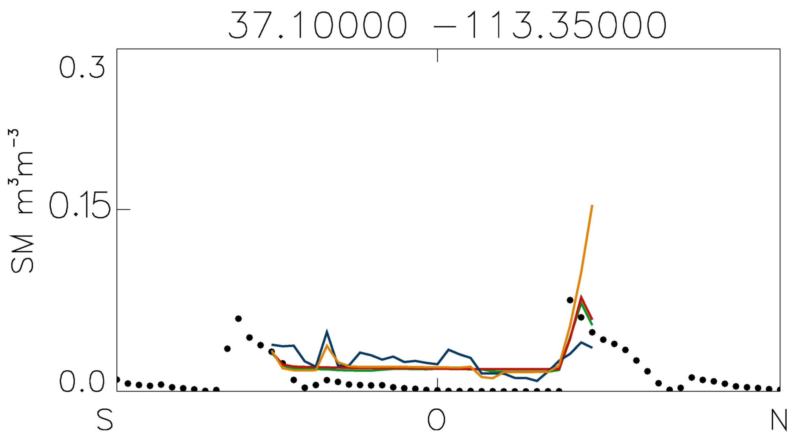
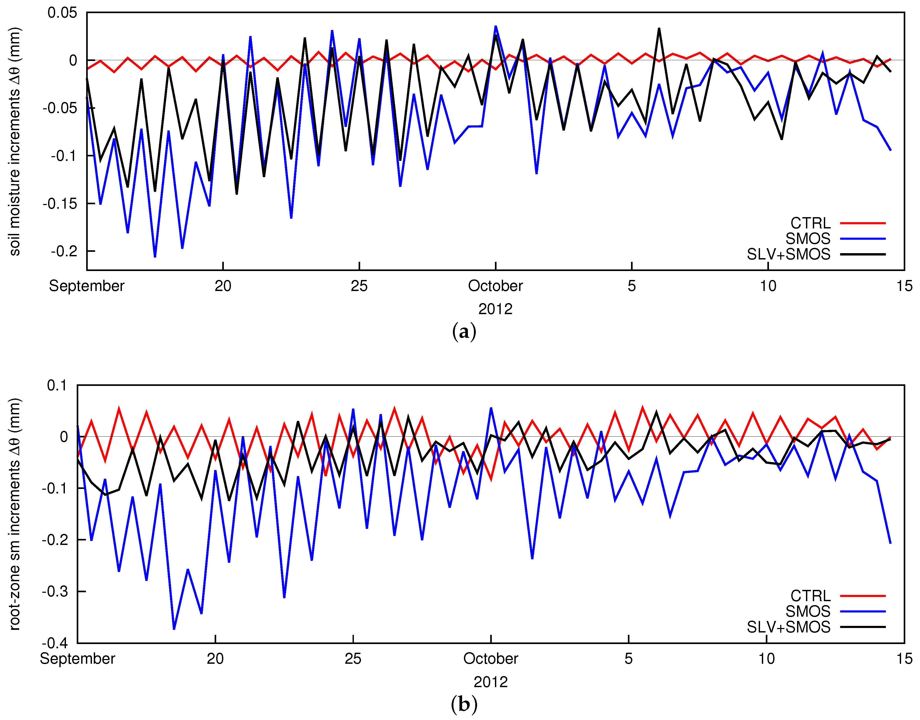
Figure 2 shows the time series of soil moisture analyses for the four experiments compared to the in situ observations, for a location where the soil is very dry and soil moisture has low variability during the studied period. It is observed that soil moisture in the SMOS experiment has larger variability compared to the other three experiments, which for this type of dry soil penalises the correlation coefficient. The large variability of the analyses in the SMOS experiment is not a good sign and it might point to too large weight of the SMOS observation in the analyses, or in other words, an underestimation of the observation error. Figure 3a shows the 12 h analysis increments averaged over the North America region for the top and root-zone layers of the experiments used in Group I. It is observed how the assimilation of SMOS T B brings much larger increments than the screen-level observations with a clear diurnal cycle. In consequence these large increments destabilize the balance of the soil, and the drying increments inferred from SMOS data are in competition with a wetter soil state reached by the land model through short model forecasts. Although the average increments are small, they produce large corrections to the soil moisture background value, which a sign of excessive weight given to the observations. The large scale spatial patterns of the increments are similar either for the SMOS or SLV+SMOS experiments (not shown), but in the former the increments can be, in absolute value, twice as large as in the SLV+SMOS experiment. The influence of SMOS observations in the root-zone is reduced, as the sensitivity to soil moisture fluctuations is confined to the top few cms. In Figure 3b, it can be seen that the SMOS increments clearly dominate the top-layer, whereas the influence of screen observations is clearly increased in the top first metre. Note also the different sign of the 00 UTC and 12 UTC increments when SMOS data is assimilated or not, meaning that both types of observations tend to add or remove water from the soil at different times.

3.1.2. Group II

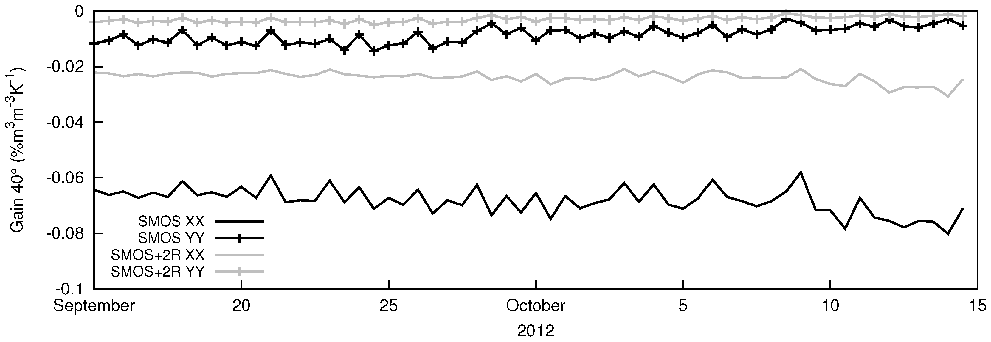
Table 3 presents the metrics for Group II of experiments. Here, the different weight assigned to the observations when only SMOS T B were assimilated was investigated. For the SCAN stations, the SMOS experiment (which assigns the specific radiometric accuracy of each observation to the observation error) obtains the lowest biases. In SMOS+2R, the weight given to the SMOS observations in the analysis is reduced and that increases biases. This is not observed over the USCRN network, where biases are similar for the SMOS and SMOS+2R experiments. As occurred in Figure 2, the unrealistic variability of the analyses in the SMOS experiment penalises the correlation coefficient and the standard deviation of the differences with ground data increases, making the ubRMSD to grow compared to SMOS+2R. By doubling the error of SMOS observations the gain is smaller, and so are the increments, as can be observed in Figure 4, either for the XX or YY polarisation. In both cases, the gain at 40° decreases significantly by doubling the observation error. This is beneficial for the correlation coefficient and the ubRMSD for just a month of analyses, although over seasonal periods the benefit should be larger. Not surprisingly, directly inserting SMOS observations (projected into model space) as replacement of soil moisture analyses obtains the worst correlation coefficient. Although in SMOS+PI unrealistically large influence is given to the observations, which should be reflected into larger increments, one should bear in mind that the SEKF quality checks still apply in this case (first-guess check, jacobian check and excessive soil moisture correction [10]), hence preventing too large spurious adjustments of soil moisture. This explains comparable bias and ubRMSD metrics with the other two experiments of this group.

3.1.3. Group III

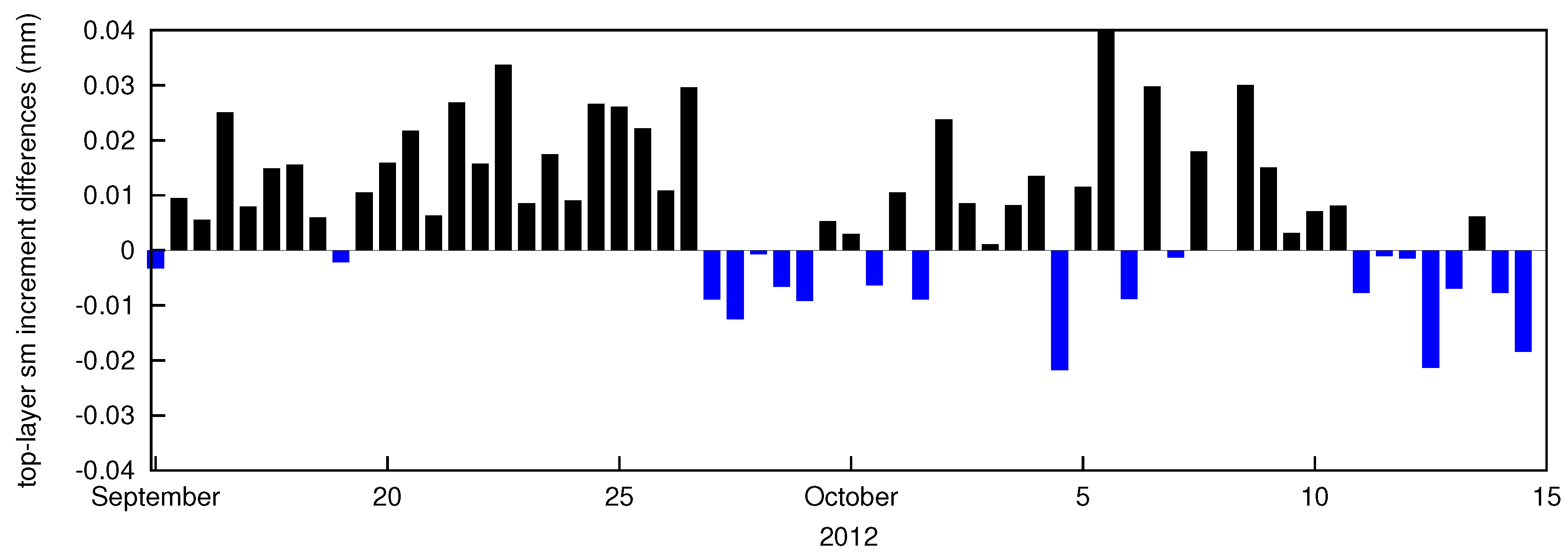
Table 4 presents the statistics for Group III of experiments, investigating the role of different definitions of the background error covariance matrix in the analysis of soil moisture. Soil physiographic parameters will either enhance or reduce the variability of soil moisture. They partly depend on soil texture, which is a key parameter of soil moisture modelling. Introducing soil texture information in the specification of the background error matrix adds realism to the error structure. In both SMOS-Btext and SMOS-3DB, soil texture information is accounted for in the uncertainty of the background error through the water holding capacity. This mainly influences the reduction of biases of the top layer compared to the SMOS experiment. On the contrary, the correlation coefficient is lower and the ubRMSD larger in SMOS-Btext and SMOS-3DB compared to SMOS and SMOS-Bprop, the latter not adding information on soil texture. In both SMOS-Btext and SMOS-3DB, the background error is implicitly increased and that increases also the gain and the increments, producing increments with stronger variability and consequent impact on the ubRMSD and correlation. The propagation of the background error covariance B depends on the linearisation of the underlying non-linear model and a constant model error, in this particular case fixed to 0.01   m 3 m 3 . In this study, the assimilation window had a length of 12 h. Compared to the SMOS experiment, SMOS-Bprop correlates slightly better with in situ data in the top soil layer. Nonetheless, the scores of both experiments are comparable due to the fact that the B matrix is reinitialized at the each cycle. This can be observed in Figure 5, as the differences are very small, lower than 0.1 mm. Cycling the B matrix at each assimilation cycle may have a positive impact over long term experiments.

3.1.4. Intercomparison of All Experiments

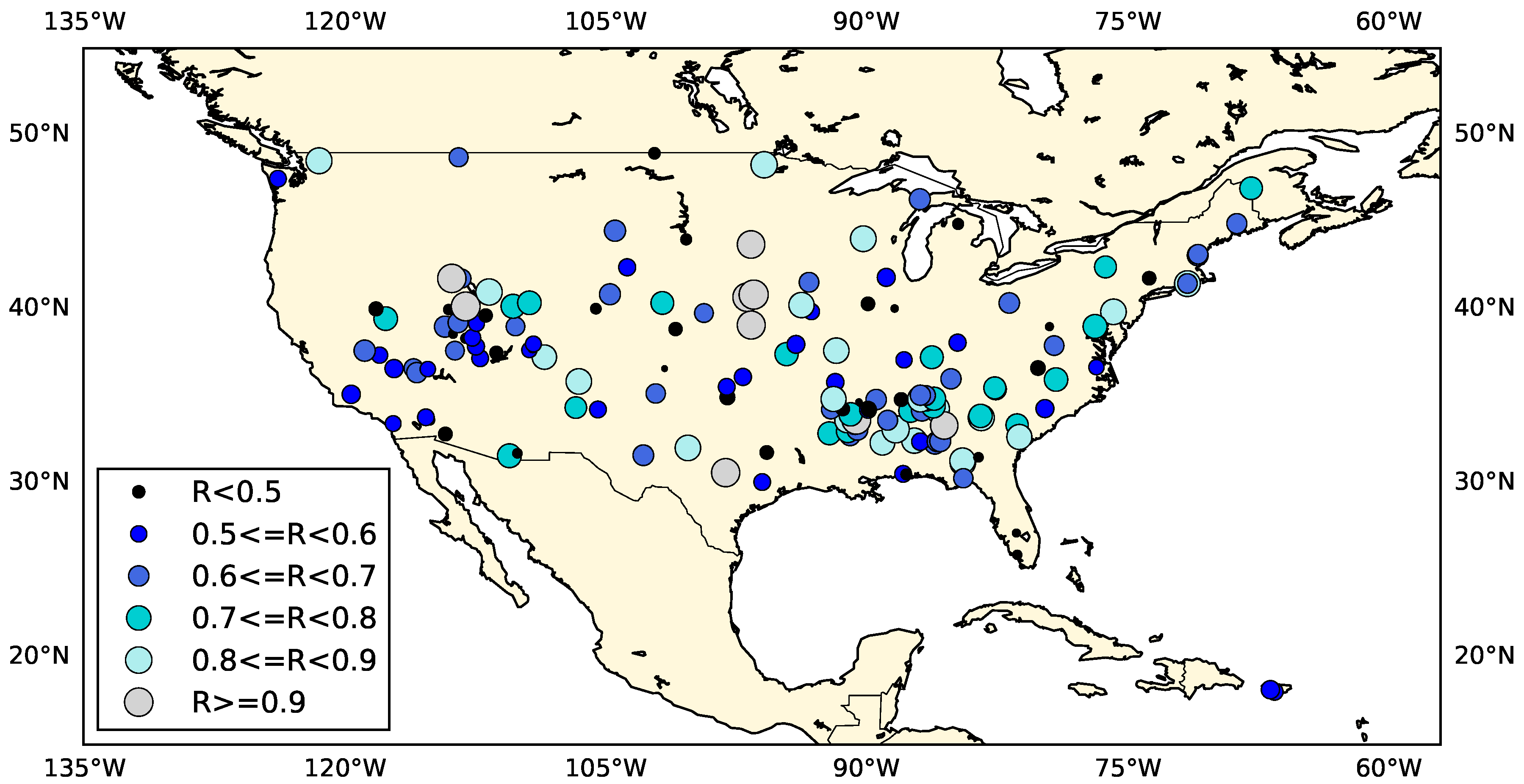
Using the same procedure for data selection as described in Section 2.4, all experiments summarized in Table 1 can be compared fairly, because the same stations are selected for each evaluation network. The immediate disadvantage, which we have to accept, is that the number of stations available is significantly reduced, only 33 out of 106 stations for the SCAN network and 28 out of 77 for the USCRN network. For both networks, SMOS+2R and SMOS+SLV obtained the best correlation scores for the top and root-zone soil moisture layer (R = 0.71 and R = 0.72, respectively). The exception is for the root-zone of USCRN, where SLV and OL were the best. The reason is partly due to the small size of the sample penalizing experiments with larger increments in a short period. For example, in Figure 6, the distribution of the SMOS experiment soil moisture analysis correlation values are shown. All stations used in the evaluation are included. The size of the circles is proportional to the correlation coefficient. This figure does not present a clear sub-regional pattern, many factors such as the meteorological conditions will influence these values too. However, a trend can be observed with more blue dots (lower correlation values) concentrated in arid or semi-arid areas in the western part of US that partly influences the averaged correlation values.
By doubling the SMOS observation error the scores were improved compared to the SMOS experiment, especially the correlation (from 0.66 (0.62) to 0.69 (0.72) for top layer (root-zone) of the SCAN network, and from 0.66 (0.65) to 0.71 (0.69) for USCRN), which is consistent with Table 3. Concerning biases, the soil moisture analyses match better the in situ observations when accounting for texture and soil depth in the background error, i.e., when increased realism is embedded in the error model of soil moisture. In all cases, a model wet bias is obtained in agreement with previous studies. For the ubRMSD, there is no clear best experiment, most of them presenting values below 0.04 m 3 m 3 , but SLV, in general, is slightly better than the rest.

3.2. Near-Surface Atmospheric Impact

3.2.1. Two-Metre Temperature and Dew Point Temperature Validation

In this section, the coupled nature of the ECMWF forecast system was exploited to investigate the impact of the soil moisture analyses in temperature and dew point temperature at 2 m above the surface.
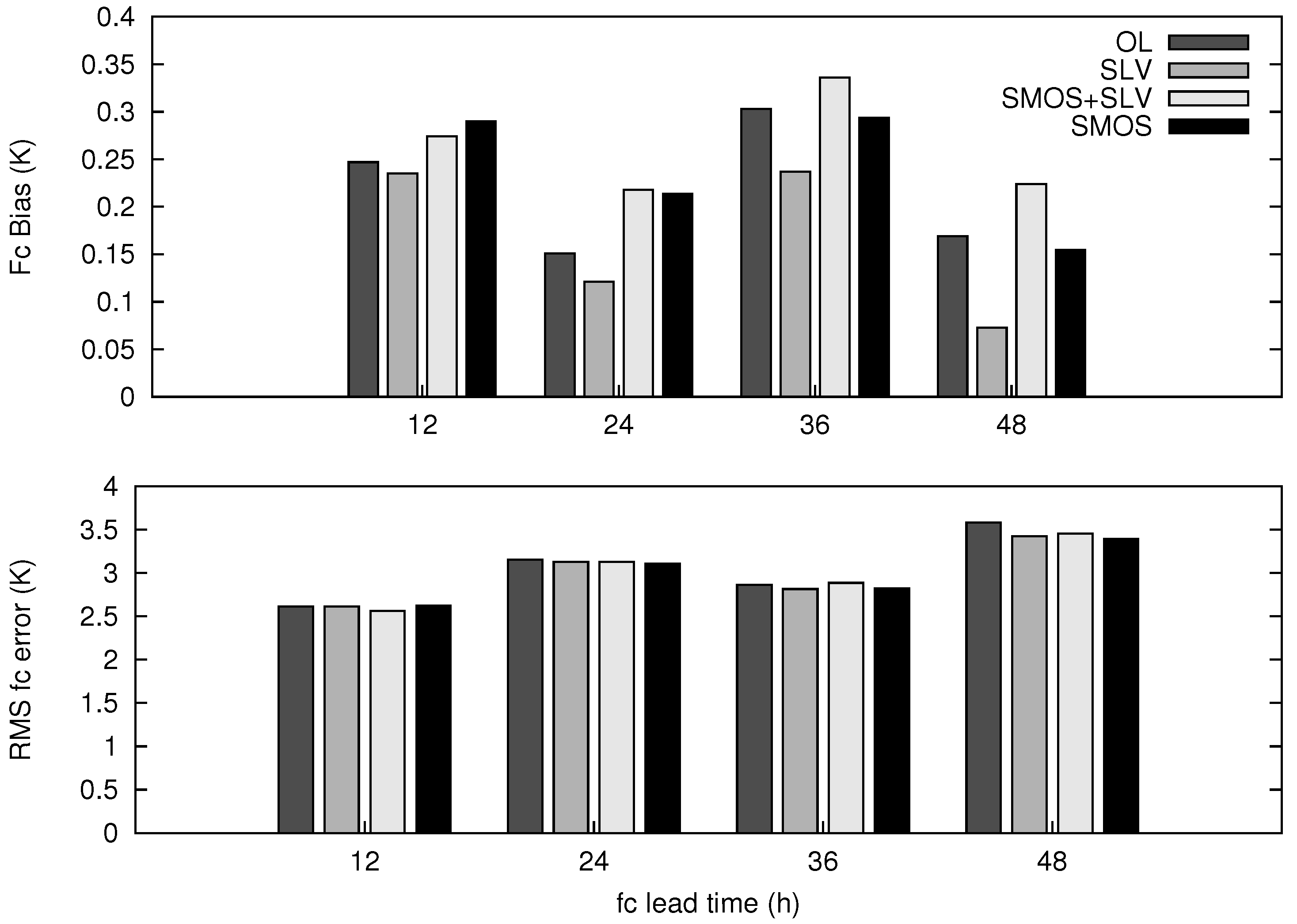
Figure 7 and Figure 8 show the forecast bias and errors as a function of four synoptic times, for 2 m dew point temperature (from which relative humidity is derived) and 2 m air temperature in Group I. The forecasts were compared against SYNOP observations, as described in Section 2.4. It is observed how forecast errors increase gradually with the forecast lead time. For 2 m dew point temperature, the model is affected by a small cold bias and/or moist bias for all four synoptic times. The SLV experiment gives the lowest biases as, indeed, the assimilation system was designed to minimize errors in screen variables. This is less apparent in 2 m temperature, where biases follow a clear diurnal cycle. A larger warm bias is observed early in the morning in North America, which is due to more stable conditions of the boundary layer, whereas biases are smaller in the evening with small vertical gradients of temperature in a well mixed boundary layer. During these experiments, SMOS makes the soil drier on average (see Figure 3), which should make the model warmer and reduce the biases. However, this is not case, suggesting that the source of these biases are others than exclusively soil moisture inaccuracies, including land surface properties, land surface modelling (possibly too few soil layers) and atmosphere–surface layer mixing in stable and unstable conditions. All these issues make the assimilation of SMOS observations challenging. For Groups II and III of experiments, small differences in 2 m temperature errors were obtained, whereas only slightly lower forecast errors of 2 m dew point temperature were obtained for SMOS+2R in Group II (not shown).

3.2.2. Near-Surface Atmospheric Scores

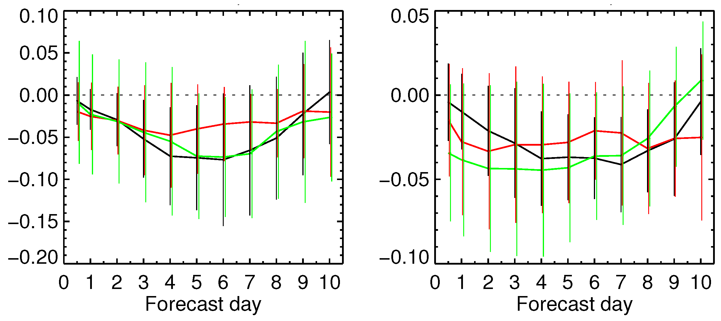
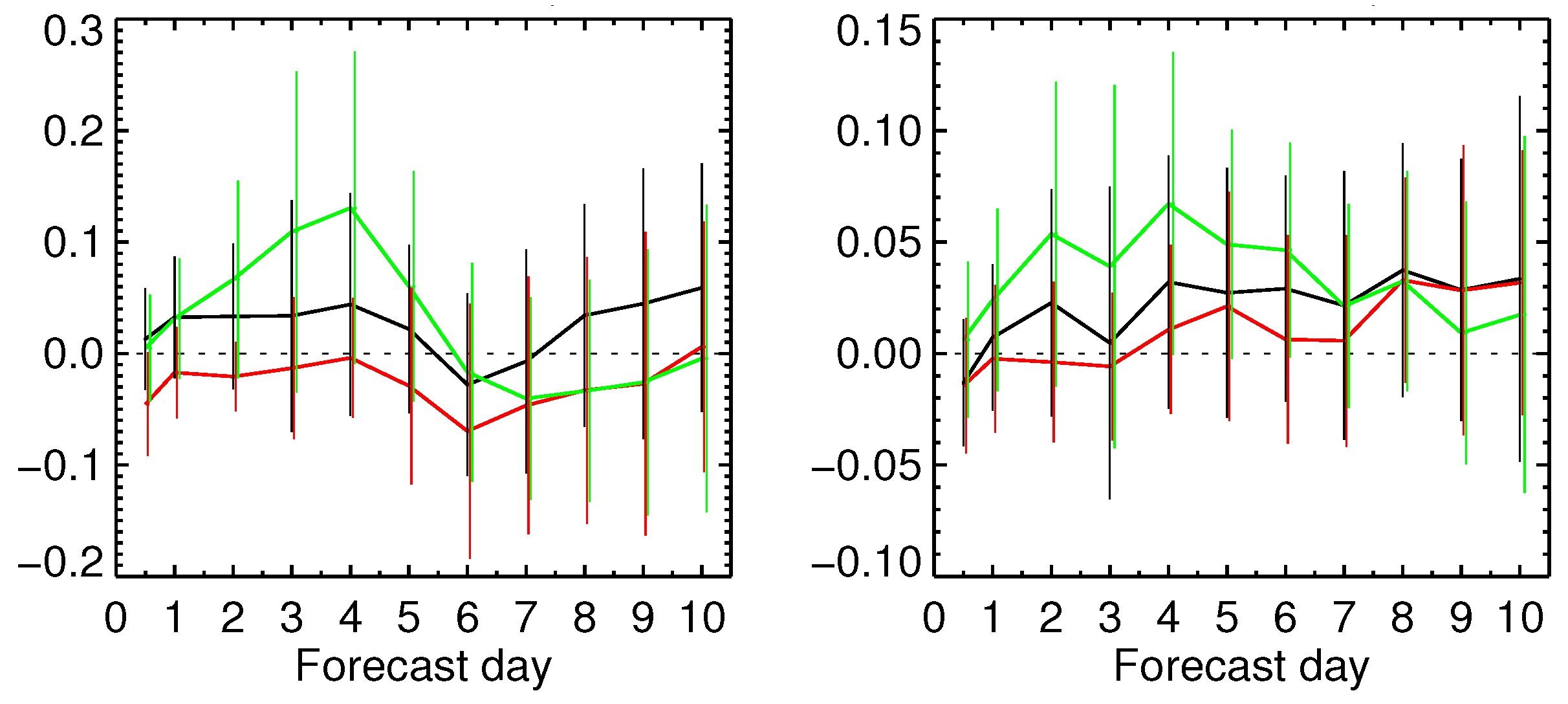
The relative forecast error of near-surface air temperature and air humidity was computed for the area under study for each experiment and up to 10 days using the operational analysis as reference given that this is the best reference available. For this type of sensitivity study, using the OL without data assimilation as reference is useful because it makes it possible to quantify the added value, if any, of assimilating screen-level or SMOS data for the soil moisture analysis. Figure 9 shows, for Group I of experiments, the root mean square forecast error normalized by the forecast error of the OL experiment. These scores are the average of 30 forecasts from 15 September to 14 October 2012. The error bars show the 95% confidence intervals. Negative values indicate that the skill of the experiment compared to the open loop simulation has increased, whereas positive values indicate a reduced skill. It is observed that all the experiments decrease the forecast error of air temperature and air humidity compared to the unconstrained forecasts, reinforcing the importance of assimilating observations sensitive to soil moisture variations in the land surface model. Statistically significant values were only obtained for the SLV experiment (black line), however the error bars are large due to the short temporal sampling. Figure 9 also shows how both experiments using SMOS data with the default observation error cannot outperform the SLV experiment, and indeed none of them reach statistical significance. In Figure 10, the experiments of Group II are compared against the skill of the SMOS experiment. In both plots, a negative impact for the first days of SMOS+PI is observed (i.e., increase of errors), which is in agreement with the results obtained for soil moisture in Table 3. The reduction of the increments in SMOS+2R have a slightly positive impact on relative humidity for the first 72 h, about 2–3% improvement. Figure 11 shows the scores obtained for Group III of experiments. In general, the skill of SMOS+Btext and SMOS+Bprop is neutral compared to the SMOS control experiment. However, the indirect increase of the background error in SMOS+3DB compared to the default value of 0.01 m 3 m 3 adds larger soil moisture increments and it has a detrimental impact on air temperature and air humidity for the first few days.

4. Summary and Conclusions

This paper presents a study of sensitivity to SMOS observation error and to background error specification, which is a crucial first step for the design of a SMOS data assimilation system. A series of one-month experiments at 40 km horizontal resolution were run assimilating screen level variables and SMOS brightness temperatures over North America, aiming at investigating the sensitivity and impact of soil moisture analysis to: (a) the type of observation assimilated in the ECMWF SEKF; (b) the confidence given to SMOS T B ; and (c) the different background error formulation. Based on the outcome of these experiments, recommendations for an operational configuration for assimilating SMOS T B and a more optimal specification of the model background error in the SEKF are presented. For the experiments to be computationally affordable, a short period had to be selected. A recharge period was selected as the temporal variability of soil moisture is larger. A consequence of the relative short assimilation period applied is that the error bars in Figure 9, Figure 10 and Figure 11 (and other similar plots) are relatively large, and therefore the scores are frequently not statistically significant. Despite the short temporal sampling, this study is very useful for identifying clear features in the sensitivity of soil moisture analysis to the use of different observations and different error configurations. The atmospheric impact of these experiments may be partly influenced by the fact that a reduced observational system to constrain the atmosphere was used. A consequence is the presence of less accurate background values which may produce large increments in the atmosphere. However, in this paper, the atmospheric impact is limited to the closest layer to the surface where this influence is minimal.
In this study, firstly, the added value of using observations sensitive to soil moisture aimed to correct its background value was highlighted. As shown in Figure 9, compared to an open loop run, the forecast of near-surface air temperature and air humidity was enhanced when SMOS T B were assimilated for the analysis of soil moisture, and the enhancement was more marked when only screen-level variables were assimilated. The latter also obtained the lowest forecast biases of 2 m dew point temperature compared to SYNOP observations. However, within each network, the soil moisture analyses scores of the OL and SLV experiments were quite similar, on average, compared to in situ data. These results can be explained by the fact that this system was initially designed to respond to (and minimize) errors of screen-level variables. On the other hand, if SMOS observations (with specific radiometric accuracy as observation error) were assimilated, no evidence of air temperature or humidity improvement was observed compared to screen-level variables. However, it did result in a closer match to soil moisture observations from US as biases were reduced in all cases, although one could argue that these results could just reflect the scale disparity between the coarse scale of the analysis and the point-scale nature of the in situ observations and therefore subjected to representativity errors. The correlation coefficient compared to in situ data were likewise degraded, but the cause of these results is due to strong increments with larger variability, which for the short period of study of this paper had detrimental consequences under dry conditions with low variability of the soil moisture time series.
Secondly, assigning the SMOS observation error to twice the radiometric accuracy had a positive impact on the temporal dynamical behaviour of the soil moisture analyses. Increasing the error of the SMOS observations produced smaller increments with lower variability, which reduces the temporal variability of the differences with soil moisture observations, particularly in dry conditions. This configuration also had a slight positive impact on air temperature and humidity. It is therefore fair to claim that the observation error used for SMOS observations was underestimated in the first group of experiments, because it only accounted for the radiometric accuracy and neglected other sources of error, such as representativeness. By giving too large confidence to the SMOS observations spurious increments were produced, which had a negative effect on both soil moisture analyses and atmospheric forecast scores.
Finally, using a background error matrix as a function of soil texture (one of the main parameters influencing soil moisture variability) had a neutral impact on the near-surface forecast. The current operational representation of the soil moisture background error is very crude, without any dependency on soil texture or on the depth of the soil. Introducing soil texture dependency on the background error increases its realism and it does not affect adversely the scores. The improvement of both SMOS-Btext and SMOS-3DB soil moisture analyses were only reflected in a reduction of biases compared to the available ground data. Differences in the root-zone were very small, yet, given the long memory of the root-zone moisture content, the potential effects of the new state of the soil on the near-surface meteorology can only be investigated over longer time scales than used in this study. In this study, propagating the background error matrix along the assimilation window did not provide evidence of any clear improvement, as the model error introduced is not cycled and is too small to have a significant effect on a 12-h assimilation window.
When all the experiments were compared using the same subset of stations, the combination of SMOS+SLV and SMOS+2R turned out to correlate better with in situ data, whereas SMOS-3DB and SMOS-Btext gave the lowest biases. The situation for the ubRMSD was more mixed and smaller values were given by OL, SLV and SMOS+2R. Although a modest tendency towards lower correlation values was observed for the experiments assimilating SMOS T B in the arid western part of US, clear sub-regional patterns of soil moisture scores were not found. Studies investigating the impact of L-band T B assimilation at local scale are complementary to this study that is more focused on the continental view as a test for using SMOS data in global NWP applications.
Therefore, the set of experiments studied in this paper suggests that the combined use of a larger observation error for SMOS observed T B data (at least doubling its radiometric accuracy) with a background error depending at least on soil texture, will be beneficial for soil moisture analyses and with a likely neutral to positive impact on the quality of near-surface atmospheric variables forecasts. These guidelines are very useful to define a configuration of the SMOS observation error and background error suitable for operational purposes. One month long experiments are sufficiently long to provide such guidelines. Figure 9, Figure 10 and Figure 11 also highlight the fact that it is worth the effort to develop our soil moisture analysis, a better initialization of soil moisture initial conditions may well result in improved lower troposphere forecasts. Further studies of the best performing configurations are planned with the full observational system and longer term experiments spanning a minimum of a whole season.

Author Contributions

J.M.-S. analyzed the data and wrote the manuscript. P.d.R. and L.I. provided a useful critical revision of the manuscript. C.A. contributed actively with the soil moisture evaluation.

Funding

This work was funded under the ESA-ESRIN contract number 4000101703/10/NL/FF/fk.

Acknowledgments

We would like to thank the SMOS mission manager S. Mecklenburg and technical officer M. Drusch (both ESA staff) for their involvement in the definition of this project. Finally, the comments of anonymous reviewers were very useful to improve this paper.

Conflicts of Interest

The authors declare no conflict of interest. The founding sponsors had no role in the design of the study; in the collection, analyses, or interpretation of data; in the writing of the manuscript, and in the decision to publish the results.

Abbreviations

ESAEuropean Space Agency
ECMWFEuropean Centre for Medium Range Weather Forecasts
IFSIntegrated Forecasting System
SMOSSoil Moisture and Ocean Salinity
NWPNumerical Weather Prediction
SEKFSimplified Extended Kalman Filter
RMSDRoot Mean Squared Difference
ubRMSDunbiased RMSD
T B Brightness Temperatures
FAOFood and Agriculture Organization
NRTNear Real Time
RFIRadio Frequency Interference
WHCWater Holding Capacity

References

  1. Shukla, J.; Mintz, Y. Influence of land-surface evapotranspiration on the Earth’s climate. Science 1982, 215, 1498–1501. [Google Scholar] [CrossRef] [PubMed]
  2. Koster, R.; Suarez, M.J. Relative contributions of land and ocean processes to precipitation variability. J. Geophys. Res. 1992, 100, 13775–13790. [Google Scholar] [CrossRef]
  3. Beljaars, A.C.M.; Viterbo, P.; Miller, M. The Anomalous Rainfall over the United States during July 1993: Sensitivity to Land Surface Parameterization and Soil Moisture Anomalies. J. Hydrometeorol. 1996, 124, 362–383. [Google Scholar] [CrossRef] [Green Version]
  4. Douville, H.; Viterbo, P.; Mahfouf, J.; Beljaars, A. Evaluation of optimal interpolation and nudging techniques for soil moisture analysis using FIFE data. Mon. Weather Rev. 2000, 128, 1733–1756. [Google Scholar] [CrossRef]
  5. Drusch, M.; Viterbo, P. Assimilation of screen-level variables in ECMWF’s Integrated Forecast System: A study on the impact of the forecast quality and analyzed soil moisture. Mon. Weather Rev. 2007, 135, 300–314. [Google Scholar] [CrossRef]
  6. Koster, R.D.; Mahanama, S.P.P.; Yamada, T.J.; Balsamo, G.; Berg, A.A.; Boisserie, M.; Dirmeyer, P.A.; Doblas-Reyes, F.J.; Drewitt, G.; Gordon, C.T.; et al. The second phase of the global land-atmosphere coupling experiment: Soil moisture contribution to subseasonal forecast skill. J. Hydrometeorol. 2011, 12, 805–822. [Google Scholar] [CrossRef]
  7. Reichle, R.; Koster, R.D.; Liu, P.; Mahanama, S.P.P.; Njoku, E.G.; Owe, M. Comparison and assimilation of global soil moisture retrievals from the Advanced Microwave Scanning Radiometer for the Earth Observing System (AMSR-E) and the Scanning Multichannel Microwave Radiometer (SMMR). J. Geophys. Res. 2007, 112, D09108. [Google Scholar] [CrossRef]
  8. Draper, C.S.; Mahfouf, J.F.; Walker, J.P. Root zone soil moisture from the assimilation of screen-level variables and remotely sensed soil moisture. J. Geophys. Res. 2011, 116, D02127. [Google Scholar] [CrossRef]
  9. Ridler, M.; Madsen, M.; Stisen, S.; Bircher, S.; Fensholt, R. Assimilation of SMOS-derived soil moisture in a fully integrated hydrological and soil-vegetation-atmosphere transfer model in Western Denmark. Water Resour. Res. 2014, 50, 8962–8981. [Google Scholar] [CrossRef] [Green Version]
  10. Muñoz-Sabater, J. Incorporation of passive microwave brightness temperatures in the ECMWF soil moisture analysis. Remote Sens. 2015, 7, 5758–5784. [Google Scholar] [CrossRef]
  11. Muñoz-Sabater, J.; Jarlan, L.; Calvet, J.; Bouyssel, F.; de Rosnay, P. From near surface to root-zone soil moisture using different assimilation techniques. J. Hydrometeorol. 2007, 8, 194–206. [Google Scholar] [CrossRef]
  12. Sabater, J.M.; Rüdiger, C.; Calvet, J.C.; Fritz, N.; Jarlan, L.; Kerr, Y. Joint assimilation of surface soil moisture and LAI observations into a land surface model. Agric. For. Meteorol. 2008, 148, 1362–1373. [Google Scholar] [CrossRef] [Green Version]
  13. Mahfouf, J.F.; Bergaoui, K.; Draper, C.; Bouyssel, F.; Taillefer, F.; Taseva, L. A comparison of two off-line soil analysis schemes for assimilation of screen level observations. J. Geophys. Res. 2009, 114, D08105. [Google Scholar] [CrossRef]
  14. Zwieback, S.; Scipal, K.; Dorigo, W.; Wagner, W. Structural and statistical properties of the collocation technique for error characterization. Nonlinear Process. Geophys. 2012, 19, 69–80. [Google Scholar] [CrossRef] [Green Version]
  15. Pierdicca, N.; Fascetti, F.; Pulvirenti, L.; Crapolicchio, R.; Muñoz-Sabater, J. Analysis of ASCAT, SMOS, in-situ and land model soil moisture as a regionalized variable over Europe and North Africa. Remote Sens. Environ. 2015, 170, 280–289. [Google Scholar] [CrossRef]
  16. Drusch, M.; de Rosnay, P.; Balsamo, G.; Andersson, E.; Bougeault, P.; Viterbo, P. Towards a Kalman filter based soil moisture analysis system for the operational ECMWF Integrated Forecast System. Geophys. Res. Lett. 2009, 36. [Google Scholar] [CrossRef]
  17. De Rosnay, P.; Drusch, M.; Vasiljevic, D.; Balsamo, G.; Albergel, C.; Isaksen, L. A Simplified Extended Kalman Filter for the global operational soil moisture analysis at ECMWF. Q. J. R. Meteorol. Soc. 2012, 139, 1199–1213. [Google Scholar] [CrossRef]
  18. Balsamo, G.; Viterbo, P.; Beljaars, A.; van den Hurk, B.; Hirschi, M.; Betts, A.; Scipal, K. A revised hydrology for the ECMWF model: Verification from field site to terrestrial water storage and impact in the Integrated Forecast System. J. Hydrometeorol. 2009, 10, 623–643. [Google Scholar] [CrossRef]
  19. Muñoz-Sabater, J.; Fouilloux, A.; de Rosnay, P. Technical implementation of SMOS data in the ECMWF Integrated Forecasting System. Geosci. Remote Sens. Lett. 2012, 9, 252–256. [Google Scholar] [CrossRef]
  20. Daley, R. Atmospheric Data Analysis; Number 2; Cambridge University Press: Cambridge, UK, 1993. [Google Scholar]
  21. Salgado, R. Global Soil Maps of Sand and Clay Fractions and of the Soil Depth for MESONH Simulation Based on FAO/UNESCO Soil Maps; Technical Report 59; CNRM: Météo, France, 1999. [Google Scholar]
  22. Lannoy, G.D.; Reichle, R. Global Assimilation of Multiangle and Multipolarization SMOS Brightness Temperature Observations into the GEOS-5 Catchment Land Surface Model for Soil Moisture Estimation. JHs 2016, 17, 669–691. [Google Scholar] [CrossRef]
  23. Lievens, H.; Tomer, S.; Bitar, A.A.; Lannoy, G.D.; Drusch, M.; Dumedah, G.; Franssen, H.; Kerr, Y.; Martens, B.; Pan, M.; et al. SMOS soil moisture assimilation for improved hydrologic simulation in the Murray Darling Basin, Australia. RSEs 2015, 168, 146–162. [Google Scholar] [CrossRef] [Green Version]
  24. Muñoz-Sabater, J.; de Rosnay, P.; Jiménez, C.; Isaksen, L. SMOS brightness temperatures angular noise: Characterization, filtering and validation. IEEE Trans. Geosci. Remote Sens. 2014, 52, 5827–5839. [Google Scholar] [CrossRef]
  25. Kerr, Y.; Waldteufel, P.; Wigneron, J.P.; Delwart, S.; Cabot, F.; Boutin, J.; Escorihuela, M.; Font, J.; Reul, N.; Gruhier, C.; et al. The SMOS mission: New tool for monitoring key elements of the Global Water Cycle. Proc. IEEE 2010, 98, 666–687. [Google Scholar] [CrossRef] [Green Version]
  26. Draper, C.; Reichle, R.; de Lannoy, G.; Liu, Q. Assimilation of passive and active microwave soil moisture retrievals. Geophys. Res. Lett. 2012, 39, L04401. [Google Scholar] [CrossRef]
  27. De Rosnay, P.; Muñoz-Sabater, J.; Albergel, C.; Isaksen, L. Comparing ERA-Interim based L-band brightness temperatures with SMOS observations: Configuration of the Community Microwave emission Modelling Platform, bias correction and SMOS long term monitoring results. 2018; unpublished. [Google Scholar]
  28. Albergel, C.; Dorigo, W.; Balsamo, G.; Muñoz-Sabater, J.; de Rosnay, P.; Isaksen, L.; Brocca, L.; de Jeu, R.; Wagner, W. Monitoring Multidecadal satellite Earth observation of soil moisture products through land surface reanalysis. Remote Sens. Environ. 2013, 138, 77–89. [Google Scholar] [CrossRef]
  29. Entekhabi, D.; Reichle, R.H.; Koster, R.D.; Crow, W.T. Performance Metrics for Soil Moisture Retrievals and Application Requirements. J. Hydrometeorol. 2010, 11, 832–840. [Google Scholar] [CrossRef]
  30. Albergel, C.; Calvet, J.; de Rosnay, P.; Balsamo, G.; Wagner, W.; Hasenauer, S.; Naeimi, V.; Martin, E.; Bazile, E.; Bouyssel, F.; et al. Cross-evaluation of modelled and remotely sensed surface soil moisture with in situ data in southwestern France. Hydrol. Earth Syst. Sci. 2010, 14, 2177–2191. [Google Scholar] [CrossRef] [Green Version]
  31. Geer, A. Significance of Changes in Medium-Range Forecast Scores; Technical Report 766; European Centre for Medium-Range Weather Forecasts: Reading, UK, 2015. [Google Scholar]
Figure 1. Region under study. Overlapped are the observations from the SYNOP network (black dots), and the ground soil moisture observations from the SCAN (red circles) and USCRN (blue circles) networks in the US.
Water 10 00890 g001
Figure 2. Soil moisture time series for the analyses of OL (red curve) SLV (green curve), SMOS (dark blue curve) and SLV+SMOS (orange curve) experiments. The daily averaged observations for this station of the SCAN network in US are displayed in black dots.
Water 10 00890 g002
Figure 3. Time series of the 12 h area averaged analysis increments of the control SLV (red curve), SMOS (blue curve) and SLV+SMOS (black curve) experiments for the: (a) top 7 cm; and (b) the root-zone layer. Note that the OL experiment is not shown here because it is not an analysis experiment.
Water 10 00890 g003
Figure 4. Averaged time series of the 40° incidence angle gain component for the SMOS and the SMOS+2R experiments.
Water 10 00890 g004
Figure 5. Top soil moisture increment differences (in mm of water) averaged over the North America region. Differences shown are SMOSSMOS-Bprop experiments.
Water 10 00890 g005
Figure 6. Correlation coefficient (R) of the SMOS experiment soil moisture analysis with in situ observations. The size of the circles is proportional to R.
Water 10 00890 g006
Figure 7. Averaged forecast biases and RMS forecast errors of 2 m dew point temperature compared to observations of the SYNOP network in North America, as a function of the forecast lead time for the four experiments of Group I.
Water 10 00890 g007
Figure 8. The same as Figure 7 but for 2 m temperature.
Water 10 00890 g008
Figure 9. Near-surface air temperature (left) and air humidity (right) normalized root mean square forecast error of SLV (black curve), SMOS (red curve) and SLV+SMOS (green curve) experiments compared to the control OL experiment, as a function of the forecast lead time. The operational analyses are used as reference. Error bars show 95% confidence intervals.
Water 10 00890 g009
Figure 10. The same as Figure 9 but for the Group II of experiments; red curve is for SMOS+2R experiment and black curve for SMOS+PI experiment compared to the control SMOS experiment.
Water 10 00890 g010
Figure 11. The same as Figure 9 but for the Group III of experiments; red curve is for SMOS+Btext experiment, black curve for SMOS+Bprop experiment and green curve is for SMOS+3DB, all compared to the control SMOS experiment.
Water 10 00890 g011
Table 1. Assimilation features of the experiments used in this study. Each column represents the following: (1) experiment name; (2) whether soil moisture is analysed? (3) whether screen level variables (SLV) are assimilated; (4) whether SMOS T B are assimilated; (5) assumed observed error standard deviation for 2 m temperature and 2 m relative humidity [ σ T 2 m , σ R H 2 m ]; (6) assumed SMOS T B observation error standard deviation (RA is the observation radiometric accuracy with typical values between 2.5–3 K), ϵ is an infinitesimal number); and (7) assumed background error standard deviation (in m 3 m 3 ). “f” represents a dependency, “ t e x t ” is soil texture, and “ d e p t h ” is the soil depth.
NameAnalysisSLVSMOS σ o SLV σ o SMOS σ b
OLnonono---
SLVyesyesno[1K, 4%]-0.01
SMOS+SLVyesyesyes[1K, 4%]RA0.01
SMOSyesnoyes-RA0.01
SMOS-Bpropyesnoyes-RA0.01
SMOS+PIyesnoyes- ϵ 0.01
SMOS+2Ryesnoyes-2 × RA0.01
SMOS-Btextyesnoyes-RA f ( t e x t )
SMOS-3DByesnoyes-RA f ( t e x t , d e p t h )
Table 2. Mean Bias, unbiased Root Mean Square Difference (ubRMSD) and time-series correlation coefficient (R) values between the in situ observations (OBS) and the expt type soil moisture analyses (AN) for USCRN and SCAN networks (OBS-AN). Only significant correlation values are used (through the p-value test with a 5% confidence interval). N is the number of stations with significant correlation values for all the experiments compared in this table. For the first metre of soil, in situ observations averaged at depth of 5, 10, 20, 50 and 100 cm were averaged and compared to the average of soil moisture analyses.
USCRNSCAN
exptBiasubRMSDRNBiasubRMSDRN
0–7 cmOL−0.1400.0310.6838−0.0630.0320.6358
SLV−0.1400.0300.6838−0.0620.0310.6458
SMOS+SLV−0.1200.0370.7038−0.0440.0350.6558
SMOS−0.1140.0340.6438−0.0310.0340.6158
0–100 cmOL−0.1040.0140.7638−0.0410.0160.6758
SLV−0.1030.0140.7538−0.0400.0160.6458
SMOS+SLV−0.1010.0140.6138−0.0380.0160.6558
SMOS−0.0920.0170.7338−0.0310.0180.5458
Table 3. The same as Table 2 but the experiment types in this table assimilate only SMOS T B with different weight given to the observations: SMOS+PI (soil moisture analysis are a direct projection of SMOS T B observation in the state space), SMOS (with the specific radiometric accuracy as the observation error) and SMOS+2R (doubling the error of the SMOS observations in the SEKF). Note that for all this group of experiments the B matrix is static.
USCRNSCAN
exptBiasubRMSDRNBiasubRMSDRN
0–7 cmSMOS+PI−0.0130.0290.5838−0.0540.0350.5749
SMOS−0.0110.0370.6138−0.0310.0360.6149
SMOS+2R−0.0110.0310.6738−0.0440.0320.6549
0–100 cmSMOS+PI−0.0960.0180.4838−0.0430.0190.5349
SMOS−0.0950.0160.5238−0.0370.0170.5349
SMOS+2R−0.0950.0160.5838−0.0390.0160.6949
Table 4. The same as Table 2 but in this table the performance of the analyses with different definitions of the B matrix is studied: in SMOS, the B matrix is fixed, whereas in SMOS-Bprop it is propagated in time until the next cycle. SMOS-Btext and SMOS-3DB introduce the information of soil texture in the background error while keeping their value fixed along the assimilation window.
USCRNSCAN
exptBiasubRMSDRNBiasubRMSDRN
0–7 cmSMOS−0.0970.0360.6241−0.0270.0360.6251
SMOS-Bprop−0.0960.0360.6441−0.0290.0360.6351
SMOS-Btext−0.0860.0420.5941−0.0150.0420.5451
SMOS-3DB−0.0850.0440.5841−0.0170.0430.5251
0–100 cmSMOS−0.0800.0150.5741−0.0290.0190.5151
SMOS-Bprop−0.0790.0160.5341−0.0280.0190.5851
SMOS-Btext−0.0790.0150.5041−0.0280.0190.5551
SMOS-3DB−0.0780.0160.4941−0.0270.0190.5151