Evaluation of Multiple Satellite Precipitation Products and Their Use in Hydrological Modelling over the Luanhe River Basin, China

Abstract

Satellite precipitation products are unique sources of precipitation measurement that overcome spatial and temporal limitations, but their precision differs in specific catchments and climate zones. The purpose of this study is to evaluate the precipitation data derived from the Tropical Rainfall Measuring Mission (TRMM) 3B42RT, TRMM 3B42, and Precipitation Estimation from Remotely Sensed Information using Artificial Neural Networks (PERSIANN) products over the Luanhe River basin, North China, from 2001 to 2012. Subsequently, we further explore the performances of these products in hydrological models using the Soil and Water Assessment Tool (SWAT) model with parameter and prediction uncertainty analyses. The results show that 3B42 and 3B42RT overestimate precipitation, with BIAs values of 20.17% and 62.80%, respectively, while PERSIANN underestimates precipitation with a BIAs of −6.38%. Overall, 3B42 has the smallest RMSE and MAE and the highest CC values on both daily and monthly scales and performs better than PERSIANN, followed by 3B42RT. The results of the hydrological evaluation suggest that precipitation is a critical source of uncertainty in the SWAT model, and different precipitation values result in parameter uncertainty, which propagates to prediction and water resource management uncertainties. The 3B42 product shows the best hydrological performance, while PERSIANN shows unsatisfactory hydrological performance. Therefore, 3B42 performs better than the other two satellite precipitation products over the study area.

1. Introduction

Precipitation is one of the most critical factors of hydrometeorological applications [1,2]. Accurate precipitation estimates play an increasingly important role in the management of water resources. In general, precipitation data can be obtained in two ways: surface-based observations and satellite and remote sensing datasets [3]. Surface-based observations are relatively straightforward and accurate; e.g, rain gauges and weather radars [4]. Generally, surface-based observations at one station are usually utilized to represent the precipitation of an area with a size of 10–100 km², especially in remote regions [5]. However, the rare and uneven networks of gauges make these observations inaccurate and unrepresentative [6]. Moreover, in some areas, such as mountainous regions, the quality of radar datasets is not high due to beam blockage, propagation errors, and vertical variability of reflectivity. On the other hand, radar data can be obtained from only limited areas [2,7,8]. However, precipitation data extracted from satellites overcome the previous problems, giving us a chance to acquire abundant precipitation information [9].

With the rapid development of satellite-based sensors and precipitation retrieval algorithms over the last decade, many satellite precipitation products have been developed. These products are used for different kinds of hydrological applications, mainly including drought warning, streamflow simulation, and flood forecasting [10,11]. The products include the United States National Aeronautics and Space Administration (NASA) Tropical Rainfall Measuring Mission (TRMM) [12], Precipitation Estimation from Remotely Sensed Information Using Artificial Neural Networks (PERSIANN) [13], Global Satellite Mapping of Precipitation (GSMap) [14], Climate Prediction Center (CPC) morphing technique (CMORPH) [15], and Multi-satellite Retrievals for Global Precipitation Measurement Mission (GPM IMERG) [16]. GPM IMERG is one of the most recent satellite precipitation products with very high spatiotemporal resolution, which is a joint effort by NASA and the Japan Aerospace Exploration Agency (JAXA). Those products generally have several versions with different spatiotemporal resolutions to meet different needs. For example, the most commonly used versions of TRMM are TRMM 3B42 (3 h-0.25°), TRMM 3B42RT (3 h-0.25°), and TRMM 3B43 (monthly 0.25°). The spatial resolution of PERSIANN is 0.25°, and the temporal resolutions of PERSIANN are 1 h, 3 h, and 6 h. The spatiotemporal resolution of the GSMap product is a 0.1°-1 h. The CMORPH products include two spatiotemporal resolution versions: 3 h-0.25° and 30 min-8 km. The spatiotemporal resolution of the final GPM IMERG product that is commonly used is a 0.1°-30 min. If precipitation products are used for flood forecasting, the temporal resolutions might be less than 6 h. In this study, we will use three satellite precipitation products (TRMM 3B42, TRMM 3B42RT and PERSIANN) because they have the same spatiotemporal resolutions (3 h-0.25°), and their temporal resolutions are less than 6 h. Then, we will plan to use three satellite precipitation products for flood forecasting. Recently, the precision of satellite precipitation products has become the focus of research because there are many uncertainties that might be caused by measurement errors, sampling, retrieval algorithms, and bias correction processes [17]. The more accurate the precipitation products, the more effective the predictions [18]. In general, quantitative statistical and hydrological modelling evaluations are two effective tools used to evaluate the precision of satellite precipitation products [19]. The purpose of the evaluation is to determine the most appropriate product to carry out other studies over a particular basin. Many researchers have explored the capabilities of numerous satellite precipitation products over many basins around the world [3,7,11,13,17,19,20,21,22,23,24,25,26,27,28]. In addition, some researchers have also evaluated multi-satellite precipitation products over some basins of China. Over the Yangtze River basin, Li et al. [29] evaluated the precipitation estimates derived from 3B42V7, CMORPH, and PERSIANN on multiple time scales, and the result showed that overall, 3B42V7 performed better than the other two products, but CMORPH was better on a daily scale. Over the Mishui basin, Jiang et al. [30] evaluated TRMM 3B42V6, TRMM 3B42RT, and CMORPH using multiple indexes and the semi-distributed Xin’anjiang model. They believed that these three products had positive potential in hydrological applications and found that 3B42V6 performed better than 3B42RT and CMORPH. In the Tibetan Plateau basin, Gao and Liu evaluated 3B42RTV6, 3B42V6, CMORPH, and PERSIANN on a daily scale [31]. They found that 3B42V6 and CMORPH performed better than 3B42V6RT and PERSIANN. Over the midlatitude Ganjiang River basin, TRMM 3B42, 3B42RT, and IMERG were quantitatively compared in the study of Tang et al. [10] over an extended period of the rainy season. The results showed that although these three products performed well with a high correlation (0.87) on grid and basin scales, and TRMM products could be adequately substituted with the IMERG product to conduct research over this area. Over the Xiang River basin and Qu River basin, Zhu et al. [32] evaluated the performance of PERSIANN-CDR, TRMM 3B42V7, and National Centers for Environment Prediction-Climate Forecast System Reanalysis (NCEP-CFSR). The results showed that 3B42V7 outperformed the other two products on a monthly scale but not on a daily scale. For hydrological applications, the 3B42V7 product performs best. To the author’s knowledge, all of the above basins are located in humid regions of south China, while there have been few evaluations over North China. The different climate regions, seasons, altitudes, storm regimes, and land surface conditions will change the error properties [28]. It is essential to assess the precision and hydrological applications of satellite precipitation products, leading to critical effects upon ecological, agricultural, and economic development. Additionally, the Luanhe River basin is a semi-arid and semi-humid climatic region of North China, and the applicability of the latest satellite precipitation products over semi-arid and semi-humid climatic regions lacks adequate coverage in the literature.

Based on this fact, the specific research objectives of this study are to (1) evaluate and compare the performance of three satellite precipitation products (TRMM 3B42RTV7, 3B42V7 and PERSIANN) on multiple time scales and spatial scale to characterize the precipitation patterns over the Luanhe River basin; (2) investigate the capability of using satellite precipitation products as inputs for the Soil and Water Assessment Tool (SWAT) model; and (3) explore their influences and prediction uncertainties of streamflow simulations.

The other sections of this article are as follows: Section 2 briefly introduces the location, the land use and soil types of the study area, geographical datasets, and satellite precipitation products. Section 3 lists the statistical metrics used for evaluating the products and provides a brief description of the SWAT model. Section 4 shows the results of a comprehensive evaluation and comparison, streamflow simulation, and uncertainty analysis for the three selected satellite precipitation products. Finally, the conclusions of this study are illustrated in Section 5.

2. Study Area and Datasets

2.1. Study Area

The Luanhe River basin is a midlatitude basin that extends from 115°30′ to 119°45′ E longitude and 39°10′ to 42°40′ N latitude in North China, with a drainage area of approximately 44,750 km². The average annual temperature and precipitation were 5–12 °C and 400–700 mm during the period from 2001 to 2012, respectively. Because 70% of the precipitation occurs during the rainy season (from May to October), the runoff has an analogous seasonality resulting in frequent floods and droughts.

The Panjiakou Reservoir was built downstream of the Luanhe River in 1983. This reservoir is one of the most important projects of the “Water Transfer from Luanhe River to Tianjin City”, playing an increasingly important role in water supply, flood control, irrigation, power, and environmental protection. Therefore, the drainage area (33,700 km²) controlled by this reservoir was selected as the study area (Figure 1a). The area has a complicated topography, significantly decreasing from northwest to southeast and an elevation ranging from 166 m to 1994 m above sea level. Mountainous regions occupy approximately 98% of the study area while plains take up approximately 2% [33]. Digital elevation model (DEM), land use, and soil data are shown in Figure 1a–c, respectively, of which the sources and descriptions are presented in the following section.

2.2. Datasets

In this study, we collected meteorological, land use and soil datasets to derive the SWAT model. The rain gauge observations were collected from the Haihe River Water Conservancy Commission (MWR). All other daily meteorological observations from four weather stations were collected from the China Meteorological Administration, including relative humidity, wind speed, maximum and minimum temperature, and solar radiation. In addition, we also obtained the available monthly streamflow observations between 2001 and 2012 from the MWR for SWAT model calibration. The distribution of all ground gauges and stations is shown in Figure 1. Digital elevation model (DEM) data with 30 m resolution were downloaded from the Geospatial Data Cloud (http://www.gscloud.cn/). The soil data downloaded from the Environmental and Ecological Science Data Center for West China, National Natural Science Foundation of China (http://westdc.westgis.ac.cn/), and the land cover data with 30 m resolution were obtained from http://www.globallandcover.com/. The soil data were reclassified into five different types according to soil texture, including loam (53.31%), clay loam (5.51%), silt loam (4.53%), sandy loam (33.42%), and sand (3.23%); the land use data were reclassified into six types according to the China Current Landuse Classification, including grasslands (19.65%), bare areas (2.20%), water (0.37%), croplands (14.54%), urban areas (1.66%), and forests (61.58%).

Meanwhile, we selected three satellite precipitation products (TRMM 3B42RTV7 (3B42RT, hereafter), TRMM 3B42V7 (3B42, hereafter) and PERSIANN), which are introduced as follows.

The 3B42RT and 3B42 products are provided by TRMM, which were launched by the National Space Development Agency (NASDA) of Japan and NASA. The products, with a 3 h temporal resolution and a 0.25° by 0.25° spatial resolution, are produced by merging calibrated passive microwave (PMW) and infrared (IR) data and calibrated by using rain gauge data from the Global Precipitation Climatology Center (GPCC) and the Climate Assessment and Monitoring System (CAMS) on a monthly scale [12]. The spatial resolution of the monthly GPCC data is 1°, and these locations are mapped in Figure 1. In this study, the data from the ground gauges in the evaluation were different from the ground gauge data derived from GPCC or CAMs. The latest versions of the 3B42RT and 3B42 products, version 7, are employed in this study, which can be freely downloaded from the NASA Goddard Earth Sciences Data and Information Services Center (GES DISC; https://mirador.gsfc.nasa.gov/). There are some differences between 3B42RT and 3B42: (1) 3B42RT is a near real-time version that can be downloaded only 9 h after real-time observations, but 3B42 is a post-real-time version that can be acquired 10–15 days after real-time observations; (2) 3B42RT is calibrated by the TRMM Microwave Imager (TMI) dataset, but 3B42 is calibrated by the TRMM Combined Instrument (TCI) dataset [27]; (3) the date range of 3B42RT is from March 2000 to present, but the date range of 3B42 is from December 1997 to present. More information is provided by Huffman and Bolvin [12].

PERSIANN products [34] are near-globally available and were developed by the Center for Hydrometeorology and Remote Sensing (CHRS) at the University of California, Irvine (UCI). The products utilize neural network procedures to compute the rainfall rate from an IR brightness temperature dataset derived from global geostationary satellites and have multi-temporal resolutions such as 3 h, 6 h, and daily. The PERSIANN parameters are calibrated by the PMW dataset because there are high levels of uncertainties due to the cloud properties and atmospheric conditions [3]. The date range of PERSIANN is from March 2000 to present, and these data can be downloaded from http://chrsdata.eng.uci.edu/.

The details of all satellite precipitation products and other necessary data are presented in

Table 1. Information of different satellite precipitation products and other datasets used in the Soil and Water Assessment Tool (SWAT) model.

Data Type	Products	Time Resolution	Time Extent	Spatial Resolution	Spatial Extent	Availability after the Events	Data Source
Meteorology	Rain gauges observations	daily	2001–2012	point	-	-	China Meteorological Administration (CMA)
	TRMM_3B42V7	3 h	31 December 1997 to present	0.25° × 0.25°	50° N to 50° S 180° E to 180° W	10–15 days	NASA Goddard Earth Sciences Data and Information Services Center (GES DISC)
	TRMM_3B42RTV7	3 h	29 February 2000 to present	0.25° × 0.25°	60° N to 60° S 180° E to 180° W	9 h	NASA Goddard Earth Sciences Data and Information Services Center (GES DISC)
	PERSIANN	3 h	1 March 2000 to present	0.25° × 0.25°	60° N to 60° S 180° E to 180° W	2 days	The Center for Hydrometeorology and Remote Sensing (CHRS) at the University of California, Irvine (UCI)
	Other Meteorological data	daily	2001–2012	point	-	-	China Meteorological Administration (CMA)
Streamflow	Hydrological station	monthly	2001–2011	point	-	-	Haihe River Water Conservancy Commission (MWR)
Geography	Digital Elevation Model (DEM)	-	-	30 m × 30 m	Luanhe River basin	-	Geospatial Data Cloud
	Land use	-	-	30 m	Luanhe River basin	-	GlobeLand30
	Soil	-	-	1 km	Luanhe River basin	-	Environmental and Ecological Science Data Center for West China, National Natural Science Foundation of China

. To evaluate the performances of the three satellite precipitation products and drive the SWAT model, all products were aggregated into daily, monthly, seasonal, and annual scales.

3. Methods

3.1. Statistical Metrics

To qualitatively evaluate precipitation data derived from three satellite products with rain gauge observations on different spatial and temporal scales, a set of widely used metrics were adopted including correlation coefficient (CC), root mean squared error (RMSE), mean absolute error (MAE) and relative bias (BIAs). The formulas for these metrics are listed in

Table 2. List of the indexes used to evaluate the overall performance of satellite precipitation products.

Index	Unit	Equation	Perfect Value
Correlation coefficient (CC)	-	$\mathrm{CC}=\frac{{{\displaystyle \sum }}_{i=1}^N(O_i-\overline{O})(S_i-\overline{S})}{\sqrt{{{\displaystyle \sum }}_{i=1}^N{(O_n-\overline{O})}^2}\sqrt{{{\displaystyle \sum }}_{i=1}^N{(S_i-\overline{S})}^2}}$	1
Root mean squared error (RMSE)	mm	$\mathrm{RMSE}=\sqrt{\frac{1}{N}{\displaystyle {\displaystyle \sum }_{i=1}^N}{(S_i-O_i)}^2}$	0
Mean absolute error (MAE)	mm	$\mathrm{MAE}=\frac{1}{N}{\displaystyle {\displaystyle \sum }_{i=1}^N}\left|(S_i-O_i)\right|$	0
Relative bias (BIAs)	%	$\mathrm{BIAs}=\frac{\frac{1}{N}{{\displaystyle \sum }}_{i=1}^N(S_i-O_i)}{{{\displaystyle \sum }}_{i=1}^N{O}_i}$	0
Coefficient of determination (R2)	-	${\mathrm{R}}^2=\frac{{({{\displaystyle \sum }}_{i=1}^N(O_i-\overline{O}){{\displaystyle \sum }}_{i=1}^N(S_i-\overline{S}))}^2}{{{\displaystyle \sum }}_{i=1}^N{(O_n-\overline{O})}^2{{\displaystyle \sum }}_{i=1}^N{(S_i-\overline{S})}^2}$	1
Nash-Sutcliffe efficiency coefficient (NS)	-	$\mathrm{NS}=1-\frac{{{\displaystyle \sum }}_{i=1}^N{(O_i-S_i)}^2}{{{\displaystyle \sum }}_{i=1}^N{(O_i-\overline{O})}^2}$	1
Probability of detection (POD)	-	$\mathrm{POD}=\frac{H}{H+M}$	1
False alarm ratio (FAR)	-	$\mathrm{FAR}=\frac{F}{H+F}$	0
Critical success index (CSI)	-	$\mathrm{CSI}=\frac{H}{H+M+F}$	1

Note: O_i, the ith pair of rain gauge precipitation (or observed streamflow); S_i, the ith pair of precipitation derived from 3B42RT, 3B42 or PERSIANN or (simulated streamflow); N: number of samples. H: the total number of correctly detected precipitation observations; M: the total number of undetected precipitation observations; F: the total number of precipitation detected but not observed.

. The CC is used to describe the linear association between satellite-based precipitation and rain gauge observations. Both RMSE and MAE are used to reflect the average magnitude of the error, but RMSE gives greater weight to larger errors than MAE. BIAs reflect the systematic bias of satellite precipitation products.

To evaluate the potential of using satellite precipitation products for rainy events at different precipitation thresholds in this study, we classified the daily rainfall amounts into four ranks: (1) rain ≤ 1 mm (no/little rain); (2) 1 mm < rain ≤ 10 mm (light/moderate rain); (3) 10 mm < rain ≤ 20 mm (low-heavy rain); and (4) rain > 20 mm (heavy rain), following Tan et al. [25]. Three categorical statistics are used to distinguish rain/no rain: probability of detection (POD), false alarm ratio (FAR), and critical success index (CSI). The formulas for these statistics are listed in Table 2 [22]. POD is used to describe the extent of rainfall events that are correctly detected; FAR reflects the extent of rainfall events that are false alarms; CSI illustrates the overall proportion of rainfall events that are correctly detected by satellite precipitation products. The perfect values for each index are mentioned in Table 2.

All three satellite precipitation products (3B42, 3B42RT and PERSIANN) have a 3 h temporal resolution. The data were added up to obtain the daily, monthly, seasonal, and annual precipitation for comparison with the gauged rainfall located within the satellite grid. The study period was from 2001 to 2012. Due to this, data derived from 3B42, 3B42RT, and PERSIANN over 12 years were roundly compared using the evaluation indexes in the study area.

3.2. SWAT Model

SWAT is a comprehensive, process-based, semi-distributed model that operates at daily time step [35]. This model contains a variety of functions including hydrological cycling, nutrient cycling, climate inputs, and crop growth, which are utilized to simulate water quantity, quality, and crop management [36,37]. There are three main steps to developing complete SWAT models for streamflow simulations, including delineating watersheds, analyzing hydrological response units (HRUs), and importing weather data.

3.2.1. Model Setup

In this study, SWAT version 2012 with ArcGIS 10.2 was used to develop the hydrological model. All datasets used in the model are listed in Table 1. First, by using DEM data, the drainage network and watershed were extracted based on an automatic procedure, and the watershed was divided into 34 sub-basins based on a drainage area threshold, which is 400 km². By imputing reclassified land use data and reclassified soil data (Figure 1), the watershed was further divided into 3864 HRUs that consist of unique combinations of soil, land use/cover, and slope. The five categories of slope were defined to be used in the HRU definitions, that is 0–2%, 2–6%, 6–15%, 15–25%, and >25%. The HRU definition adopted multiple HRU methods. The percentages of land use over sub-basin, soil class over land use area, and slope class over soil class were 0, 0, and 0, respectively. Finally, meteorological data were obtained from four meteorological stations and precipitation data were derived from satellite precipitation products while rain gauges were used to set up a weather database.

3.2.2. Model Calibration, Validation, and Uncertainty Analysis

The SWAT Calibration and Uncertainty Program (SWAT-CUP) tool was used for SWAT model sensitivity, calibration, validation, and uncertainty analysis [38]. There are five algorithms in this software, including Particle Swarm Optimization (PSO), Sequential Uncertainty Fitting Version 2 (SUFI-2), Generalized Likelihood Uncertainty Estimation (GLUE), Parameter Solution (Parasol), and Markov Chain Monte Carlo (MCMC). The SUFI-2 algorithm was used in this study for selecting sensitive parameters, calibration, and validation because it is stable and easy to operate; the algorithm aims at obtaining the uncertainty values of all parameters and tries to collect observed data within the 95% prediction uncertainty (95PPU) of the model, which was calculated through Latin hypercube sampling [39]. The selected sensitive parameters and their initial ranges recommended by SWAT official documentation [40] and other studies are listed in

Table 3. Information of SWAT parameters and initial ranges for calibration.

Parameters	Unit	Description	Calibration Range
r_CN2.mgt	-	Initial soil conservation service runoff	[−0.3, 0.3]
v_ALPHA_BF.gw	days	Baseflow alpha factor	[0, 1]
v_GW_DELAY.gw	days	Groundwater delay	[0, 500]
v_GWQMN.gw	mm	Threshold depth of water in the shallow aquifer required for return flow to occur	[0, 5000]
v_GW_REVAP.gw	-	Groundwater “revap” coefficient	[0.02, 0.2]
v_ESCO.hru	-	Soil evaporation compensation factor	[0.01, 0.1]
v_CH_N2.rte	-	Channel hydraulic conductivity	[0, 0.3]
v_ALPHA_BNK.rte	-	Baseflow alpha factor for bank storage	[0, 1]
r_SOL_AWC().sol	-	Available soil water capacity	[−0.95, 0.95]
r_SOL_K().sol	mm/h	Saturated hydraulic conductivity of the soil	[−0.95, 0.95]

Note: v_, the parameter value is replaced by a given value; r_, the parameter value is multiplied by a given value.

[26,39,41]. Before calibration, we selected common sensitive hydrological parameters and their initial ranges recommended by SWAT official documentation [40] and the literature [26,33,39,40,42]. The one-at-a-time SWAT-CUP [39] procedure is used for the sensitivity analysis to select the sensitive parameters among common sensitive hydrological parameters. This procedure tests the model sensitivity by modifying one parameter while keeping all other parameters unchanged [26]. More details can be found in the official SWAT-CUP documentation [39]. Furthermore, the models were calibrated using the initially selected sensitive parameter ranges with four iterations, and 1000 simulations were run at each iteration according to the official SWAT-CUP documentation [39]. The ranges of the parameters were replaced by the new parameters that were recommended by the program and the reasonable physical ranges.

In addition, the SUFI-2 algorithm provides ten objective functions to evaluate the model performance, such as coefficient of determination (R²), Nash-Sutcliff (NS) efficiency coefficient [43], and mean square error (MSE). In this study, R² and NS were used to evaluate the model performance. The details of these two indexes are provided in Table 2. R² measures the similarity of the observed time series and predicted time series trends, and the optimal R² value is 1. NS shows the degree of deviation between the observations and predictions. According to Chen et al. [44], the model performance can be classified into four ranks by using R²: unsatisfactory (R² ≤ 0.60), satisfactory (0.60 < R² ≤ 0.75), good (0.75 < R² ≤ 0.85), and excellent (R² > 0.85). In addition, there are also four classifications when using NS: unsatisfactory (NS ≤ 0.50), satisfactory (0.5 < NS ≤ 0.70), good (0.70 < NS ≤ 0.80), and excellent (NS > 0.80). The parameter uncertainty analysis of SUFI-2 is formed not by a single signal, but certain ranges of parameters based on the theory that the 95PPU represents the model performance. In addition, to quantify the uncertainties of the prediction, two metrics were used: R-factor and P-factor, of which the values lower than 1.5 and higher than 0.7, respectively, are acceptable in terms of discharge. The R-factor is the width of the 95PPU band, and the P-factor is the fraction of measured data within the 95PPU band. More information can be found in Abbaspour et al. [39].

The goal of calibration is to obtain the best simulation that matches the observed natural streamflow for certain forcing data. However, different inputs to a hydrologic model can highly affect the model outputs because they have biases compared with the unknown true values and bring uncertainty for hydrological models [45]. In this study, we calibrated the sensitive parameters with individual satellite precipitation products as model inputs, considering the potential effects of input uncertainty on calibration and the streamflow simulations [30,46]. The observed monthly streamflow (2001–2012) data from hydrological stations were used for calibration and validation. The first two years (2001–2002) were the warm-up period, and the period from 2003 to 2007 was the calibrated period; the period from 2008 to 2012 was the validated period.

4. Results and Discussions

4.1. Evaluation of Satellite Precipitation Products Against Gauge Observations

In this section, the performances of satellite precipitation products against gauged precipitation observations are evaluated over the basin. To investigate precipitation characteristics, the comparative analysis is conducted over 12 years, and the results are demonstrated as follows.

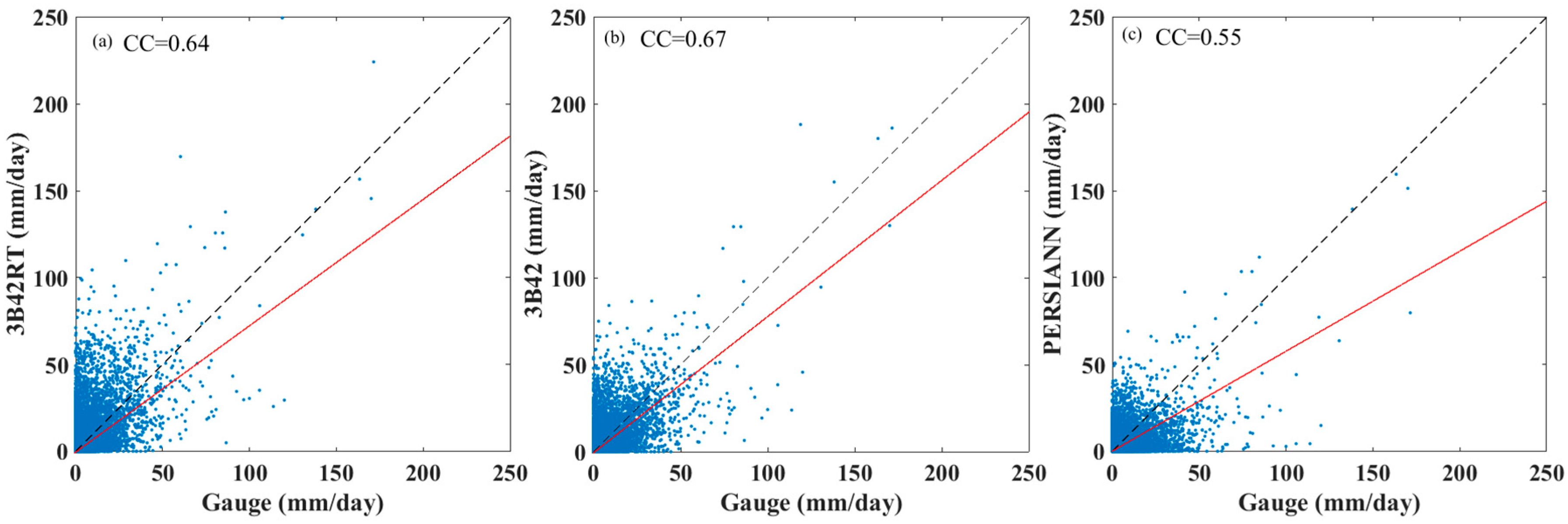
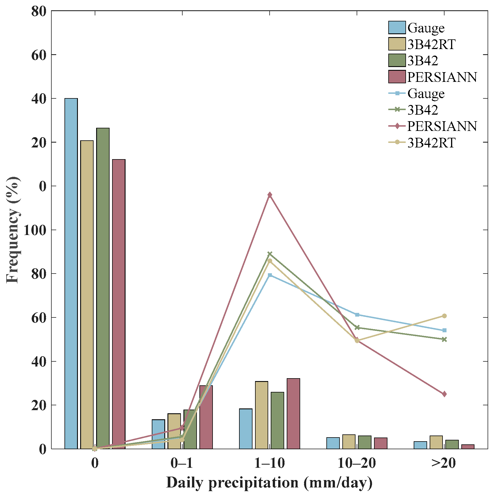
4.1.1. Daily Comparison

To assess the three precipitation products, this paper compared the satellite grids with the gauged rainfall located directly within the grid. The limited number of rain gauges in the basin might bring uncertainty [10]. The scatter plots of the daily 3B42RT, 3B42, and PERSIANN products compared to the rain gauge data are shown in Figure 2. Then, we calculated the statistics.

Table 4. Average indexes of rain gauge observations and satellite precipitation products both on daily and monthly time scales.

Time Scale	Precipitation Types	Mean (mm)	RMSE (mm)	MAE (mm)	CC	BIAs (%)	POD	FAR	CSI
Daily	Gauge	1.36	-	-	-	-	-	-	-
	3B42RT	2.20	5.91	1.77	0.64	62.80	0.75	0.29	0.74
	3B42	1.63	4.60	1.36	0.67	20.17	0.79	0.24	0.78
	PERSIANN	1.27	4.79	1.53	0.55	−6.38	0.63	0.37	0.62
Monthly	Gauge	41.55	-	-	-	-	-	-	-
	3B42RT	67.21	49.34	30.29	0.86	62.80	-	-	-
	3B42	49.85	21.91	13.08	0.94	20.17	-	-	-
	PERSIANN	38.63	30.82	19.68	0.80	−6.38	-	-	-

lists average indexes for daily comparisons. In general, 3B42 (Figure 2b) overestimates precipitation (BIAs: 20.17%), and B42RT (Figure 2a) seriously overestimates precipitation (BIAs: 62.80%), but PERSIANN (Figure 2c) underestimates precipitation (BIAs: −6.38%). Because 3B42 has a post-real-time bias adjustment, it effectively reduced the biases from 62.80 to 20.17% over the basin, as shown in Table 4. The RMSE (4.6 mm/day) and MAE (1.36 mm/day) for 3B42 are the best. The CC of 3B42 is higher than that for 3B42RT and PERSIANN. In addition, the results of the indexes for 3B42RT are not positive among the three satellite precipitation products. These results imply that 3B42 has a stronger correspondence with gauge observations than PERSIANN, followed by 3B42RT on a daily scale.

To explore the performance of satellite precipitation products detecting rainfall events, categorical statistics (POD, FAR and CSI) are usually employed, and the threshold for no rain/rain is 1 mm/day in this study (Table 4). As shown, these three products have high values (>0.63) of POD and CSI and low values (<0.37) of FAR, which means that these products are able to correctly detect and distinguish many more rainfall events. However, these three satellite precipitation products miss some events or report false events. The FAR values of 3B42RT, 3B42, and PERSIANN are 0.29, 0.24, and 0.37, respectively. Therefore, these values may lead to the poor detection of precipitation extents and intensities. Generally, among these three satellite precipitation products, 3B42 performs the best and has the highest POD (0.79) and CSI (0.78) and the lowest FAR (0.24) values. By contrast, the PERSIANN product has the lowest POD and CSI values of 0.63 and 0.62, respectively, and the highest FAR values of 0.37. These results illustrate that 3B42 can detect more precipitation events than 3B42RT, followed by PERSIANN.

The occurrence frequencies of different rainfall events from daily gauge observations, 3B42RT, 3B42, and PERSIANN and their relative contributions to the total rainfall during the period 2001–2012 are shown in Figure 3. Overall, these three products underestimate the occurrence of no rain events (rain = 0 mm), while they overestimate both the occurrence frequencies and contributions of little rain and light/moderate rain (0 ≤ rain ≤ 10 mm). PERSIANN deviates most significantly for no/little rain events, light/moderate rain events, and heavy rain events both in occurrence frequency and contribution. The better performance of TRMM (3B42RT and 3B42) results from the improvement of the bias of these satellite precipitation products on a monthly scale [12]. There are no significant differences in the occurrence frequencies of low-heavy rain events among these products. When comparing their contributions with the gauge observations, PERSIANN illustrates the largest discrepancy, while 3B42 and 3B42RT are very similar to the gauge observations. In fact, 3B42 deviates less than the other two products for the occurrence frequencies and contributions of all rainfall intensities, as shown in Figure 3. For example, 3B42 estimates the occurrence frequency of no rain events to be approximately 73%, which is approximately 7% lower than the actual occurrence frequency; however, this estimation is the best among the three satellite precipitation products. Moreover, 3B42 estimates the occurrence frequency of light/moderate rainfall events to be approximately 15%, which is approximately 6% higher than the actual occurrence frequency but is the best among the three satellite precipitation products.

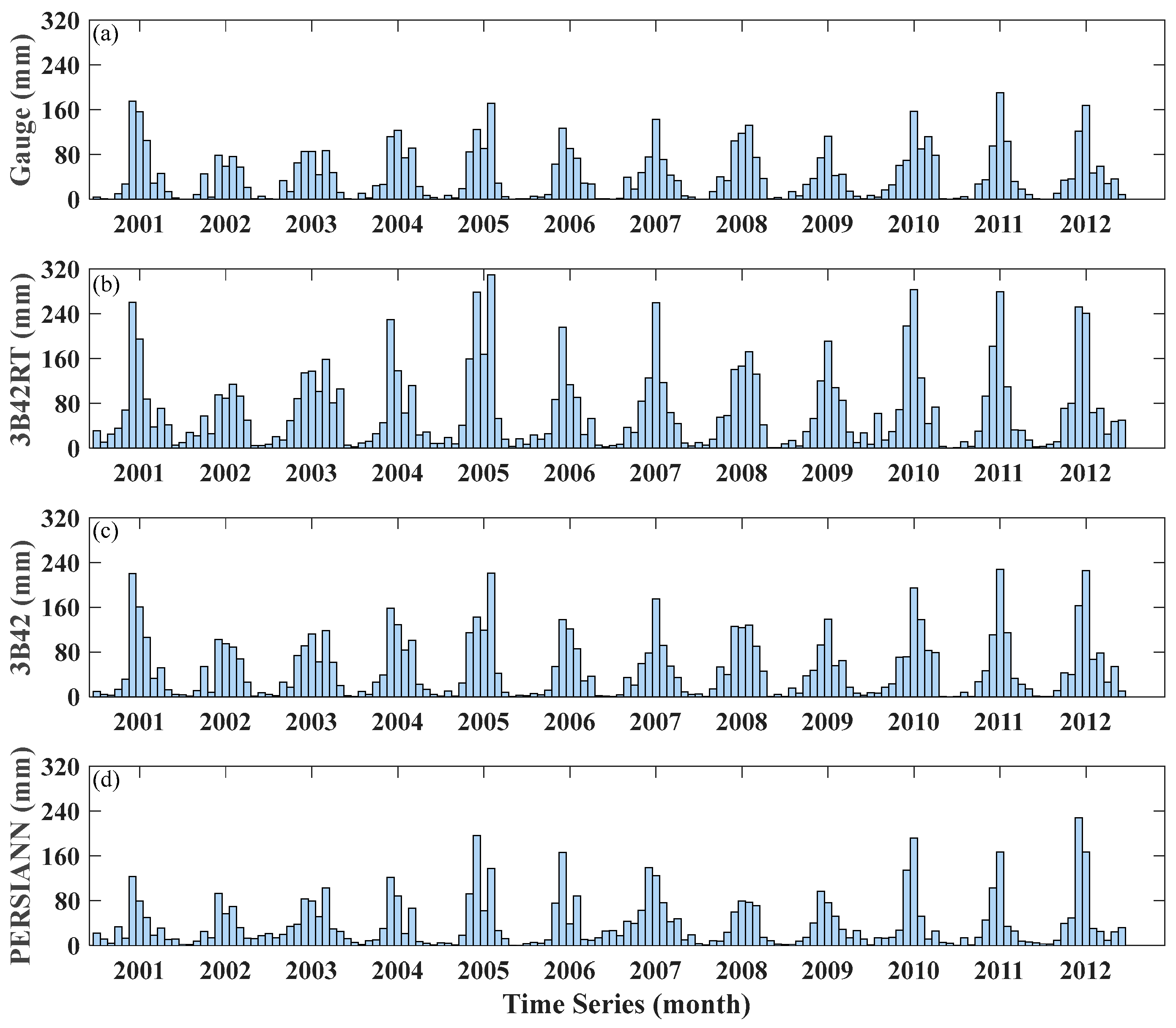
4.1.2. Monthly Comparison

To evaluate these three products directly on a monthly scale, the average monthly time series of precipitation events in the basin derived from gauges, 3B42RT, 3B42, and PERSIANN during the period 2001–2012 are shown in Figure 4. It is clear that similar results are obtained, and 3B42RT seriously overestimates precipitation, while PERSIANN slightly underestimates precipitation. The 3B42 product is illustrated to have a similar time series with a sufficient CC of 0.94 compared to rain gauge observations. Based on the average indexes of gauge observations and satellite precipitation products on a monthly time scale, as shown in Table 4, 3B42 has the best RMSE (21.91 mm/month), MAE (13.08 mm/month), and CC (0.94) values, and PERSIANN has the best BIAs (−6.38%) values, while all the indexes of 3B42RT are negative. In addition, the monthly comparisons show much higher CC values with the observations than the daily comparisons. This result largely results from errors in the daily values offset to some extent when added to the monthly values. Overall, we consider that 3B42 exhibits overall better performance than PERSIANN, followed by 3B42RT when analyzed according to the monthly time series (Figure 4) and evaluation statistics (Table 4).

To further obtain the comprehensive error contributions, the spatial distributions of the metrics (CC, RMSE and BIAs) on a monthly scale are computed using an inverse distance weighted (IDW) technique. Figure 5a–c show that the CC values of 3B42RT, 3B42, and PERSIANN increase from the north to the south of the basin. However, the RMSE values (Figure 5d–f) also increase from the north to the south, which is probably because the rain gauges are mainly concentrated in the south of the basin. The distributions of 3B42-BIAs and PERSIANN-BIAs (Figure 5h,i) show tendencies that are similar to the RMSE, but 3B42RT-BIAs (Figure 5g) on both sides of the south region are lower than those throughout the basin and the distribution trend is not similar to those of the other metrics.

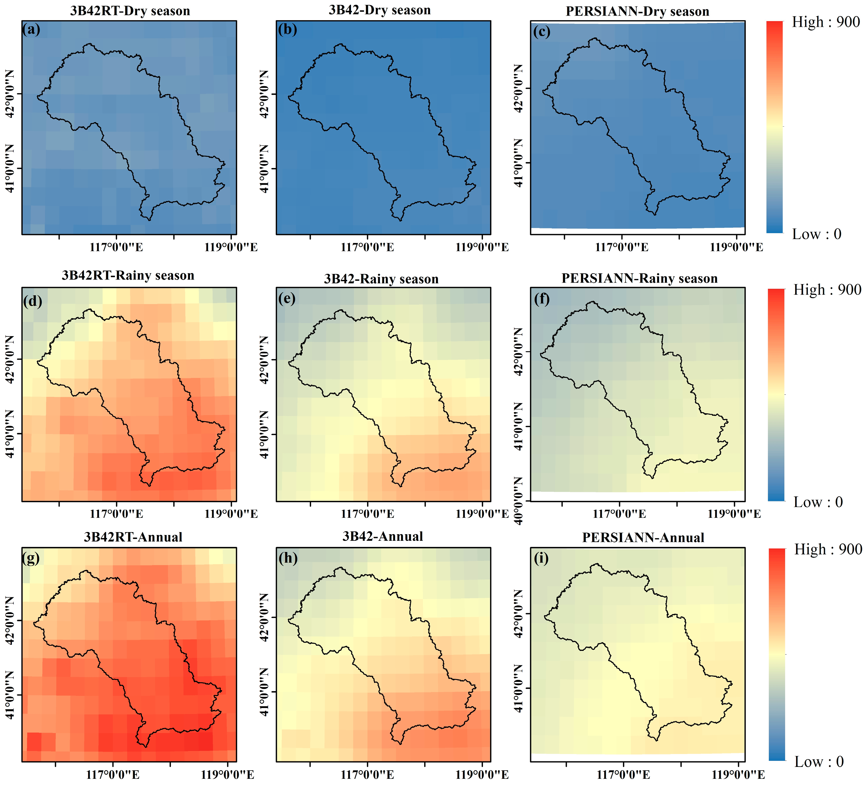
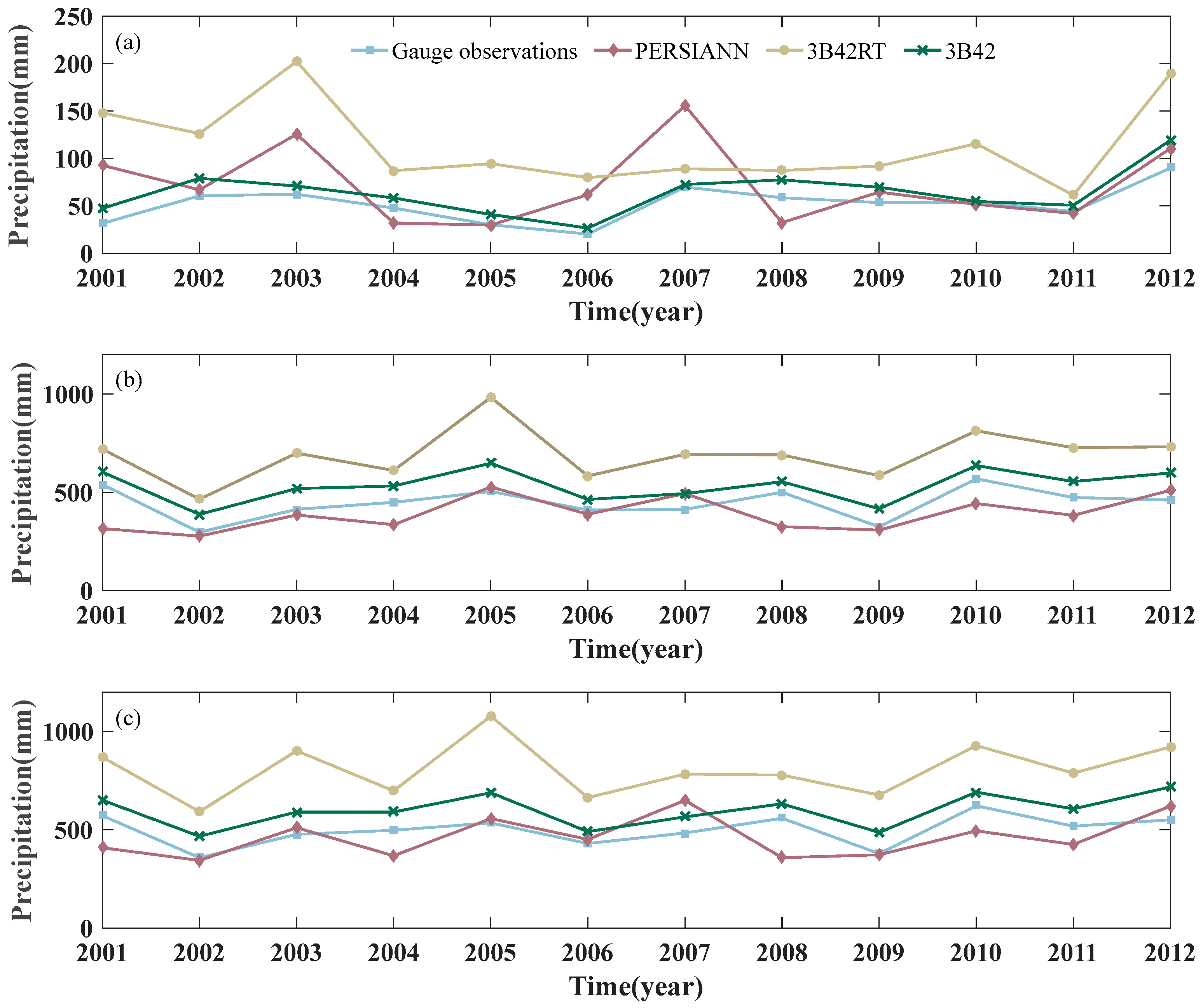
4.1.3. Seasonal (Rainy/Dry Spells) and Annual Comparisons

Evaluating satellite precipitation products on seasonal and annual scales is of great significance. In the study area, much precipitation occurs during May to October, so these six months are defined as the rainy season, and the other six months within the year are defined as the dry season to verify the performance of satellite-based precipitation products in this study. Finally, the annual performances of the satellite-based precipitation products are evaluated for managing water resources. In fact, over the basin, the average annual precipitation values for the dry season, rainy season, and the entire year are 51.87, 446.68 and 498.55 mm/year, respectively, which are calculated using rain gauge observations from 2001 to 2012. Figure 6 illustrates the spatial distribution of the average annual precipitation (mm/year) derived from 3B42RT, 3B42, and PERSIANN for the dry season, rainy season, and the entire year.

For the seasonal (dry/rainy) comparison, it is easily noted that the precipitation estimates from 3B42RT for the dry season and rainy season (Figure 6a,d) are higher than those from the other two products. For the rainy season, the spatial precipitation patterns of the three products are similar, with the precipitation intensities increasing from the northern part to the southern part of the basin, which is consistent with the spatial patterns of annual precipitation. However, the spatial precipitation patterns for the dry seasons of these three products are distinct with different intensity distributions. The important feature from the seasonal (dry/rainy) comparisons is that the 3B42 and PERSIANN estimates better match the actual precipitation values than 3B42RT for the dry season and rainy season.

For the annual comparison, it is clearly shown in Figure 6g–i that the precipitation intensities gradually increase from the high-latitude regions (northern part) to low-latitude regions of the basin (southern part). In addition to the apparently higher precipitation amounts estimated by 3B42RT, the spatial distribution patterns of precipitation from 3B42 and PERSIANN are relatively similar. In fact, when comparing the results with the actual average annual precipitation, which is approximately 498.55 mm/year, 3B42 performs better than PERSIANN because PERSIANN slightly underestimates the actual precipitation. Overall, the precipitation patterns of 3B42 and PERSIANN are more visually compatible than that of 3B42RT, and the results are similar to the results of the daily and monthly comparisons.

To further explore the annual performances of the three products, the time series of the dry season, rainy season, and total annual precipitation (mm/year) from the rain gauge observations, and 3B42RT, 3B42, and PERSIANN estimates from 2001 to 2012 are shown in Figure 7. The 3B42RT product (light yellow line) seriously overestimates precipitation when compared to the rain gauge observations (light blue line) of the total precipitation during the dry season, rainy season, and the entire year. For the PERSIANN product, there is not a clear relationship with the gauge observations, and it sometimes overestimates or underestimates the actual precipitation in the dry season, rainy season, or the entire year. For instance, the total amount of precipitation (Figure 7a, light red line) from the PERSIANN product is higher or lower than the actual precipitation (light blue line), and it is higher than the actual precipitation in 2001 while it is lower in 2008. The 3B42 estimates (light green) are slightly higher than the actual precipitation but exhibit a similar tendency, which performs well, as illustrated above.

In summary, the daily, monthly, seasonal, and annual evaluation analyses indicate that these three satellite precipitation products (3B42RT, 3B42, and PERSIANN) perform well in comparison to the rain gauge observations over the study area during the period from 2001 to 2012. However, 3B42 is better than PERSIANN, followed by 3B42RT because 3B42 has much higher CC, POD, and CSI values, lower RMSE and FAR values, and a relatively low MAE value. Meanwhile, 3B42 is able to capture the temporal and spatial distribution patterns of precipitation better than the other two products over the study basin. The 3B42 product is a good alternative to rain gauges for hydrometeorological research applications.

4.2. Hydrological Evaluation

In this section, the three satellite precipitation products on a daily scale were used as inputs to drive a SWAT model to simulate runoff. In addition, the model was then calibrated using SWAT-CUP against the observed streamflow at the outlet of the study area. Due to the lack of observed daily streamflow, only the monthly streamflow at the hydrological station was used to evaluate the capabilities of using 3B42RT, 3B42, and PERSIANN for streamflow simulations.

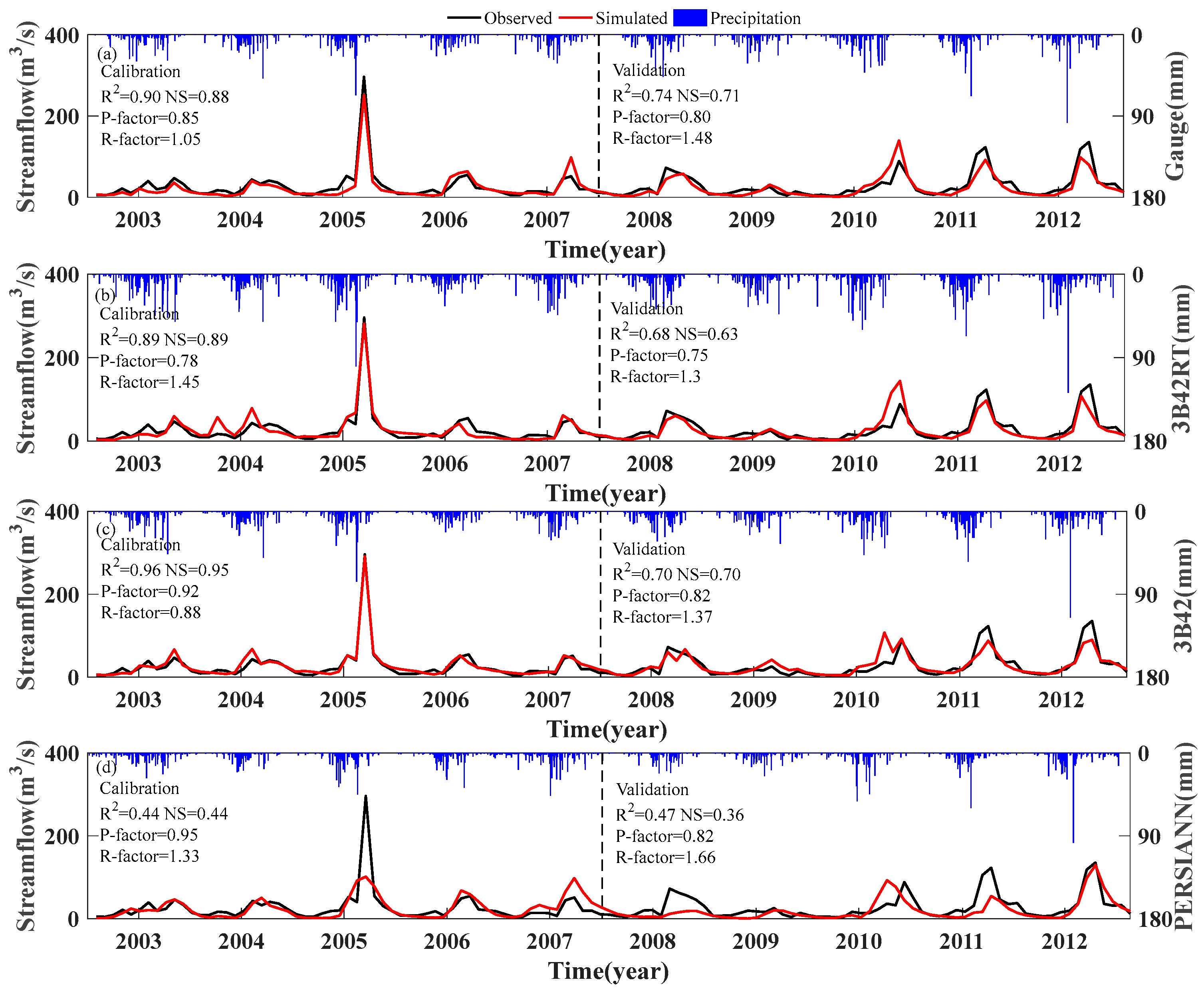
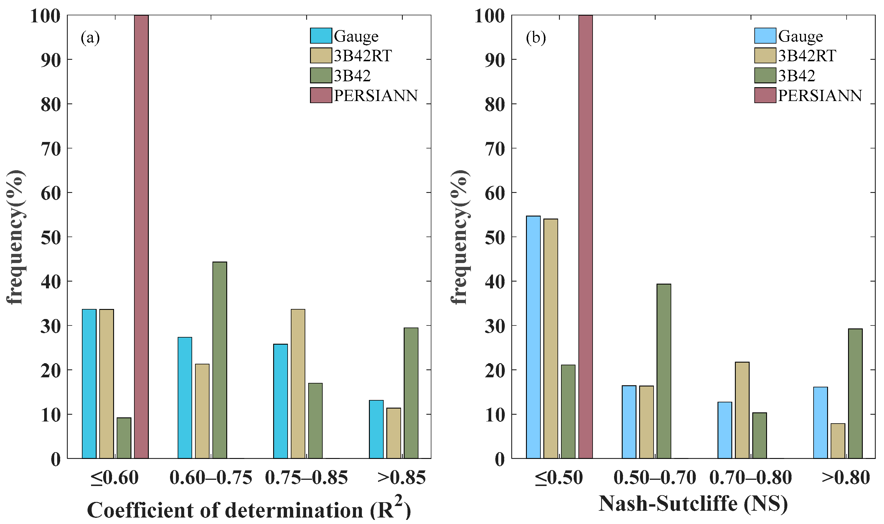
4.2.1. Hydrological Modelling Performance

The SWAT simulation results with different precipitation inputs from rain gauge observations and 3B42RT, 3B42, and PERSIANN estimates were calibrated and validated using SWAT-CUP. The period of calibration is from 2003 to 2007, and the period of validation is from 2008 to 2012.

The comparisons of the observed and simulated streamflow from the rain gauge observations and the three satellite precipitation products with the best NS, R², P-factor and R-factor results for both the calibration and validation periods are shown in Figure 8. In the study area, the simulated streamflow reproduced by the different precipitation inputs from the rain gauge observations and the 3B42RT and 3B42 estimates adequately matched the observed streamflow, while the performance of PERSIANN was not satisfactory, and the results were also evaluated in terms of the objective functions. The models using the rain gauge observations and the 3B42RT and 3B42 estimates as the precipitation data attain excellent performance during the calibration period (NS = 0.88, 0.89 and 0.96, respectively), and good performance during the validation period (NS = 0.71, 0.86 and 0.70, respectively), while the performance of the model with the PERSIANN data is unsatisfactory for both the calibration and validation periods (NS = 0.44 and 0.36, respectively). The highest NS values are reached when using the 3B42 input data during the calibration period and when using the rain gauge observations during the validation period. For the coefficient of determination R², during the calibration period, all the models forced by the rain gauge, 3B42RT, and 3B42 data exhibit excellent performance (R² > 0.89), and during the calibration period, these three models exhibit satisfactory performance (R² > 0.6). The 3B42 data-forced model exhibits the highest R² value (R² = 0.96). However, the PERSIANN data-forced model does not attain satisfactory performance (R² < 0.6). Furthermore, we use the simulated streamflows of rain gauge, 3B42RT, 3B42 and PERSIANN data-forced model and observed streamflow for linear fitting, and the fitting equations for these models were y = 0.83x + 0.72 (R² = 0.83), y = 0.81x + 1.77 (R² = 0.80), y = 0.85x + 1.01 (R² = 0.86), and y = 0.49x + 4.50 (R² = 0.42), respectively. The simulated streamflows of rain gauge, 3B42RT, 3B42 data-forced model can fit better than that of PERSIANN data-forced model because the slopes of their fitting equations are close to 1 and the intercepts are relatively small, as well as R² are larger than 0.80. On the contrary, the fitting equation of simulated streamflows of PERSIANN data-forced model has a relatively smaller slope (0.49) and R² (0.42), and larger intercept (4.50). It is clear that the performance of 3B42 data-forced model is the best, while the performance of PERSIANN data-forced model is not acceptable.

In summary, the good performance of the gauge data-forced model means that the SWAT model is capable of simulating streamflow over the study area. The better performances of the TRMM 3B42RT and 3B42 data-forced models probably result from the monthly bias adjustments, and these models might capture the occurrence of most rainfall days, especially those with heavy rainfall (Figure 3) although they overestimate precipitation at different levels. The poor performance of the PERSIANN data-forced model might have resulted from (1) PERSIANN underestimates precipitation, as discussed in Section 4.1; therefore, it cannot correctly reproduce the extreme events, that can also be seen in Figure 8 (blue bars); i.e., it cannot represent the high flow during the rainy season in 2005; (2) the SWAT system is uncertain, which might result in errors from the PERSIANN inputs. There are some techniques to improve the performance of satellite precipitation products in hydrologic models, such as data assimilation. The data assimilation approach can be used for improving the accuracy of hydrological simulations [47]. The ensemble Kalman filter (EnKF) is a technique that can be used for data assimilation [48]. A new method for data assimilation was proposed by Javaheri et al., and more details of this method can be found in the literature [47].

Beside the visual and statistical evaluations of the best simulations of the gauge observations and all satellite precipitation products, we also assessed the ensemble simulations of all gauge and satellite precipitation products. The frequencies of R² and NS values obtained at the final calibration (1000 simulations) and validation (1000 simulations) iterations are calculated. In other words, for each precipitation input, there are 2000 simulations available for the frequency calculation. Figure 9 shows the frequency of R² (a) and NS (b) values at the different classifications described above. Over the study area, both R² and NS values of all results are unsatisfactory for the PERSIANN data-forced model, while the other three models exhibit relatively good performance. In terms of R², approximately 66% of the gauge and 3B42RT data-forced model results are at the satisfactory/good/excellent level, and 90% of the 3B42 data-forced model results are at the satisfactory/good/excellent level. Moreover, the 3B42 data-forced model shows the largest fraction (approximately 30%) with excellent performance (R² > 0.85). Meanwhile, the proportions of gauge, 3B42RT, and 3B42 simulations with NS > 0.5 are 55%, 56%, and 80%, respectively. In addition, the 3B42 data-forced model achieves the highest percentage (approximately 30%) of excellent performance with NS > 0.80. Thus, the precipitation from 3B42 not only leads to the best model performance with the highest R² and NS values in both the calibration and validation periods but also contributes to the best set of model simulations among the 3B42RT, 3B42, and PERSIANN precipitation products. To some extent, the performance of the 3B42 data-forced model is even better than that of the gauge data-forced model.

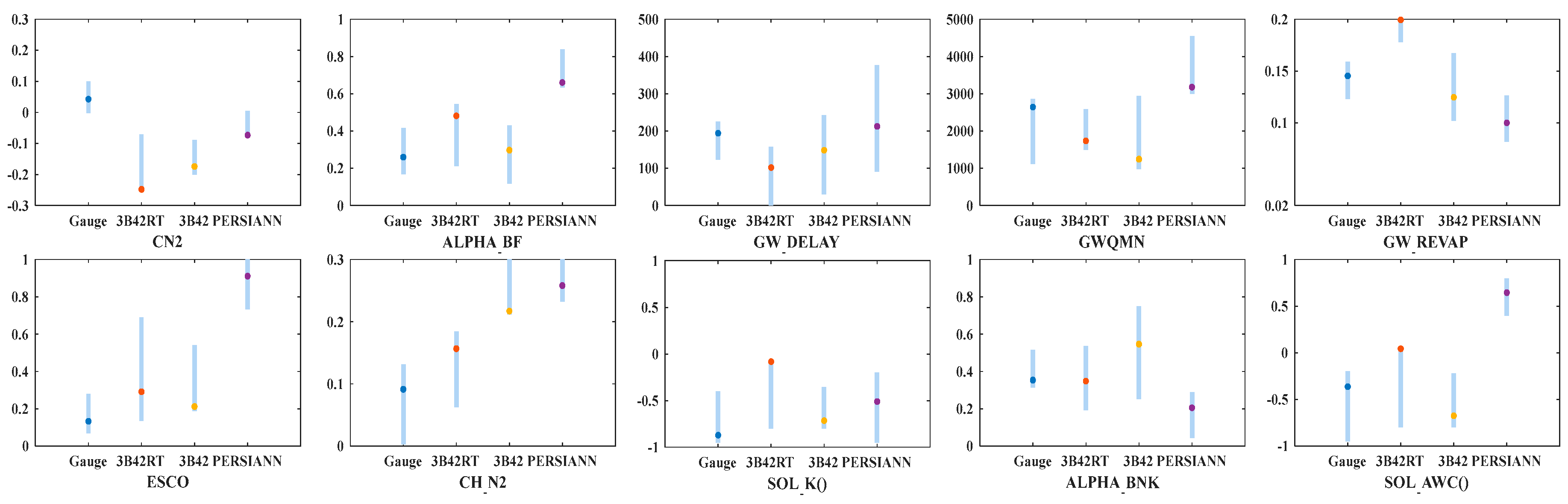
4.2.2. Parameter Uncertainty

In this study, four precipitation inputs derived from the gauge, 3B42RT, 3B42, and PERSIANN data were used to force the SWAT model. The models are capable of adjusting relevant sensitive parameters and converging to different parameter intervals to reproduce the streamflow that matches the observed streamflow.

In general, CN2 is one of the most sensitive parameters among all hydrological parameters, which represents the surface runoff generated by precipitation [26]. If precipitation inputs are different, the best CN2 value and range are different for the different models. For instance, the best-fit r_CN2 values for the rain gauge data-forced model is 0.04 while that for the 3B42RT data-forced model is −0.25 (Figure 10). Nonetheless, it is impossible to identify similar patterns for the different basins, and as a result, there are no certain patterns between the calibrated CN2 ranges and the different precipitation inputs, even in the different study areas [26]. SOL_AWC, which is responsible for available soil water capacity, is also affected by changes in precipitation. The best-fit values of r_SOL_AWC for the gauge, 3B42RT, 3B42, and PERSIANN data-forced model are −0.4, 0, −0.8 and 0.7, respectively (Figure 10). In addition, ESCO is a soil evaporation compensation factor that reflects the evaporation ability of soil, which is affected by both different precipitation inputs and different study areas. The best-fit values of v_ ESCO for the gauge, 3B42RT, 3B42, and PERSIANN data-forced model are not the same, which are 0.1, 0.3, 0.2 and 0.9, respectively. GW_DELAY is an important hydrological parameter that reflects the delayed time of groundwater. Because the precipitation inputs are not the same, the best GW_DELAY values and ranges also differ. And the best values and uncertainty ranges of other sensitive parameters, like ALPHA_BF, GWQMN, GW_REVAP, CH_N2, ALPHA_BNK, and SOL_K, are also different because the precipitation inputs are different, as shown in Figure 10. Generally speaking, due to the use of different precipitation inputs, the best values and uncertainty ranges of parameters are different, which causes the parameters uncertainty.

In fact, a visual inspection of Figure 10 reveals that the best-fit values of all sensitive parameters and their optimal ranges are influenced by the different precipitation inputs derived from gauge, 3B42RT, 3B42, and PERSIANN data. There is no clear pattern to identify the precipitation input that has larger or smaller parameter uncertainty. Moreover, if the study basin changes, the sensitive parameters and their ranges will also change [26]. In fact, SWAT-CUP adjusts the parameters that can change the water volume of different hydrological components, such as runoff depth, in order to match the observed streamflow. Therefore, even though the models can capture the pattern of observed streamflow (Figure 8), the redistribution of the single flow is not the same. As shown in

Table 5. The annual simulation results of the different water balance components during the period from 2003 to 2012.

Satellite Precipitation Products	Water Components	Period (Year)
		2003	2004	2005	2006	2007	2008	2009	2010	2011	2012
Rain gauge	Total precipitation (mm)	461	480	489	494	464	541	322	612	451	522
	Evapotranspiration (mm)	296	312	282	270	246	315	220	313	269	263
	Runoff depth (mm)	66	70	90	77	73	83	57	102	86	89
3B42RT	Total precipitation (mm)	875	634	1086	619	749	726	643	869	745	810
	Evapotranspiration (mm)	536	446	587	471	446	415	415	494	413	503
	Runoff depth (mm)	59	77	120	49	59	65	71	64	70	80
3B42	Total precipitation (mm)	562	558	594	461	502	611	406	647	533	643
	Evapotranspiration (mm)	446	399	368	353	363	372	276	319	327	330
	Runoff depth (mm)	62	68	93	55	56	81	64	95	84	90
PERSIANN	Total precipitation (mm)	526	385	516	436	623	356	364	479	416	573
	Evapotranspiration (mm)	468	335	381	335	467	322	322	359	352	440
	Runoff depth (mm)	46	38	66	44	68	34	29	65	44	76

, although different precipitation inputs affect the best estimate and uncertainty range of the parameters, the main hydrological compartments (such as evapotranspiration, runoff depth) have similar water volumes. For instance, over the study area, the calibrated rain gauge data-forced model has higher optimal CN2 ranges (Figure 10) than the other three models. This result indicates that when facing similar rainfall, the gauge data-forced model produces more surface runoff than the other three models. The calibrated PERSIANN data-forced model has a higher GWQMN value than the other models, which affects groundwater management practices, reflecting the different groundwater processes compared to other three models. In addition, the calibrated PERSIANN data-forced model has a high ESCO value in comparison to the other three models, which shows higher soil evaporation [49]. As a result, different precipitation input leads to parameter uncertainty, and further propagates to prediction uncertainty (Table 5).

4.2.3. Prediction Uncertainty

Parameter uncertainties also propagate to the prediction uncertainties of hydrological models [36]. Here, only the prediction uncertainty of streamflow is discussed, which is illustrated by the P-factor and R-factor (Figure 8). Over the study basin, in the calibration period, all the models acquire reasonable uncertainties, with P-factors higher than 0.78 and R-factors narrower than 1.5 [39]. Among the four models, the 3B42 data-forced model shows the smallest prediction uncertainties with a relatively high P-factor (0.92) and the smallest R-factor (0.88). In terms of the validation period, the P-factor and R-factor values are satisfactory for all models except the PERSIANN data-forced model (R > 1.5). In general, all four models illustrate acceptable prediction uncertainties, as shown by a comprehensive balance between the P-factor and R-factor. In particular, the 3B42 data-forced model also performs best in comparison to the 3B42RT and PERSIANN data-forced models and is even better than the gauge data-forced model.

Table 5 provides information about the annual simulation results of the different water balance components during the period from 2003 to 2012, such as total precipitation (mm), evapotranspiration (mm) and runoff depth (mm). The total precipitation of the model outputs is almost equal to the results in Figure 7. The total precipitation of the 3B42RT data-forced model output is the highest. The total precipitation of the 3B42 data-forced model output is slightly higher than that of the rain gauge data-forced model output, but these models maintain similar tendencies. The total precipitation of the PERSIANN data-forced model output fluctuates around the rain gauge data-forced model output. In addition, it is clear that the higher the total precipitation, the higher the evapotranspiration among the outputs of the different precipitation data-forced models. Furthermore, the runoff depth of the PERSIANN data-forced model output is clearly lower than that of the other three data-forced model outputs. The runoff depth of the 3B42 data-forced model output is closer to that of the rain gauge data-forced model output compared with the 3B42RT data-forced model output. Therefore, the outputs of the SWAT models enforced by different precipitation data are different, which illustrates the uncertainty of the model prediction. After calibrating the models, the 3B42 data-forced model was found to have a runoff depth that was similar to the rain gauge data-forced model.

In summary, only the PERSIANN data-forced model obtained unacceptable R-factor values in the validation period, while the other models in both the calibration and validation periods obtained acceptable P-factors and R-factors. In addition, the 3B42 data-forced model has the smallest prediction uncertainty. However, this result cannot be applied to other basins because the prediction uncertainties of gauge and satellite precipitation products are different in different study areas. Overall, different precipitation datasets will result in parameter uncertainty, further causing prediction uncertainties and even resulting in different water resource management decisions [49]. The different precipitation data-forced models have different outputs of the water balance components. As discussed above, calibrating the four models with different precipitation inputs contributes to the different best-fit parameters and ranges (i.e., the calibrated parameter ranges of the gauge, 3B42RT, 3B42, and PERSIANN data-forced models may not overlap). In addition, the best three simulations for each model are explored, and all models have R² > 0.68 and NS > 0.63, except the PERSIANN data-forced model. This result suggests that the critical input parameter is the precipitation.

5. Conclusions

In this study, we comprehensively evaluated the applicability and reliability of satellite precipitation products (3B42RT, 3B42 and PERSIANN) over the Luanhe River basin, North China during the period from 2001 to 2012.

(1) Several critical findings of the statistical comparison of the 3B42RT, 3B42, and PERSIANN products are listed as follows:

On a daily scale, all precipitation products derived from 3B42RT, 3B42, and PERSIANN show good correspondence (CC > 0.55) with gauge precipitation. In particular, the CC of 3B42 is higher than those of 3B42RT and PERSIANN, which is 0.67. Meanwhile, 3B42 and PERSIANN show better performance than 3B42RT in terms of all statistical indexes. In addition, 3B42RT overestimates precipitation, and 3B42 slightly overestimates precipitation, while PERSIANN shows slight underestimation. When comparing precipitation data from satellites and gauges to distinguish different rain events, the three products exhibit relatively accurate detection over the study area. Among all products, the occurrence frequency of 3B42 matches better with the gauge observations than 3B42RT, followed by PERSIANN. In other words, when detecting the rainfall events, the TRMM products perform better than the PERSIANN product due to the monthly gauge adjustment procedure. In addition, the similar conclusions can be discovered from POD, FAR, and CSI scores.

When evaluating 3B42RT, 3B42, and PERSIANN on a monthly scale, conclusions that are similar to those on the daily scale are obtained: 3B42RT seriously overestimates precipitation, but PERSIANN slightly underestimates precipitation. Meanwhile, 3B42 exhibits a variation trend that is similar to that from the monthly averaged gauge observations. The monthly CC values for all products are higher than the daily CC values. The monthly CC values of all products increase from the north to the south of the basin, with the RMSE increasing based on the spatial distribution of the monthly statistical metrics.

The spatial variations of the 3B42RT, 3B42 and PERSIANN products exhibit similar tendencies in the rainy season and on the annual scale, but not during the dry season. This variation shows that precipitation is higher in the north (high latitude) and lower in the south (low latitude) of the Luanhe River basin. Among these three products, the 3B42 and PERSIANN products match the gauge observations better than 3B42RT, which overestimates precipitation and shows the highest spatial fluctuations, especially on the dry seasonal scale.

(2) In terms of the hydrological evaluation, the SWAT model was forced by precipitation derived from the gauge, 3B42RT, 3B42, and PERSIANN data to examine their hydrologic utilities. The model with precipitation data from rain gauges showed good R² and NS values during both the calibration and validation periods, which means that the SWAT model is capable of simulating the streamflow over the study area. The 3B42 data-forced model performs better than the 3B42RT data-forced model, while the PERSIANN data-forced model shows unsatisfactory performance. As a result, the 3B42RT and 3B42 products are positive sources for streamflow simulations over the Luanhe River basin.

(3) When the hydrological model is forced by different precipitation inputs (gauge, 3B42RT, 3B42 and PERSIANN), the calibrated parameter ranges and the best-fit parameter set will change, which shows the uncertainty of the model parameters, causing prediction uncertainty that can be seen from the different outputs of the water balance components of the simulation result. Controlling prediction uncertainty plays an important role in hydrological applications and water resource management. In this study, all models have acceptable P-factors and R-factors except the PERSIANN data-forced model, which has an unacceptable R-factor during the validation period. In particular, the runoff depth of the 3B42 data-forced model output is generally similar to that of the rain gauge data-forced model, and it shows the smallest prediction uncertainty. In fact, the hydrological modelling performance of 3B42 is best among the three satellite products and even better than the gauge data-forced model.

References

1. Kidd, C.; Huffman, G. Global Precipitation Measurement. Meteorol. Appl. 2011, 18, 334–353. [Google Scholar] [CrossRef]
2. Hou, A.Y.; Kakar, R.K.; Neeck, S.; Azarbarzin, A.A.; Kummerow, C.D.; Kojima, M.; Oki, R.; Nakamura, K.; Iguchi, T. The Global Precipitation Measurement Mission. Bull. Am. Meteorol. Soc. 2014, 95, 701–722. [Google Scholar] [CrossRef]
3. Alijanian, M.; Rakhshandehroo, G.R.; Mishra, A.K.; Dehghani, M. Evaluation of Satellite Rainfall Climatology Using CMORPH, PERSIANN-CDR, PERSIANN, TRMM, MSWEP Over Iran. Int. J. Climatol. 2017, 37, 4896–4914. [Google Scholar] [CrossRef]
4. Ma, Y.; Zhang, Y.; Yang, D.; Bin Farhan, S. Precipitation Bias Variability Versus Various Gauges Under Different Climatic Conditions over the Third Pole Environment (TPE) Region. Int. J. Climatol. 2015, 35, 1201–1211. [Google Scholar] [CrossRef]
5. Chao, L.; Zhang, K.; Li, Z.; Zhu, Y.; Wang, J.; Yu, Z. Geographically Weighted Regression Based Methods for Merging Satellite and Gauge Precipitation. J. Hydrol. 2018, 558, 275–289. [Google Scholar] [CrossRef]
6. Strauch, M.; Kumar, R.; Eisner, S.; Mulligan, M.; Reinhardt, J.; Santini, W.; Vetter, T.; Friesen, J. Adjustment of Global Precipitation Data for Enhanced Hydrologic Modeling of Tropical Andean Watersheds. Clim. Chang. 2017, 141, 547–560. [Google Scholar] [CrossRef]
7. AghaKouchak, A.; Behrangi, A.; Sorooshian, S.; Hsu, K.; Amitai, E. Evaluation of Satellite-Retrieved Extreme Precipitation Rates Across the Central United States. J. Geophys. Res. Atmos. 2011, 116, D02115. [Google Scholar] [CrossRef]
8. Yang, T.; Feng, L.; Chang, L. Improving Radar Estimates of Rainfall Using an Input Subset of Artificial Neural Networks. J. Appl. Remote Sens. 2016, 10, 026013. [Google Scholar] [CrossRef]
9. Kidd, C.; Levizzani, V. Status of Satellite Precipitation Retrievals. Hydrol. Earth Syst. Sci. 2011, 15, 1109–1116. [Google Scholar] [CrossRef] [Green Version]
10. Tang, G.; Zeng, Z.; Long, D.; Guo, X.; Yong, B.; Zhang, W.; Hong, Y. Statistical and Hydrological Comparisons between TRMM and GPM Level-3 Products over a Midlatitude Basin: Is Day-1 IMERG a Good Successor for TMPA 3B42V7? J. Hydrometeorol. 2015, 17, 121–137. [Google Scholar] [CrossRef]
11. Sun, R.; Yuan, H.; Liu, X.; Jiang, X. Evaluation of the Latest Satellite-Gauge Precipitation Products and their Hydrologic Applications over the Huaihe River Basin. J. Hydrol. 2016, 536, 302–319. [Google Scholar] [CrossRef]
12. Huffman, G.J.; Bolvin, D.T. TRMM and Other Data Precipitation Data Set Documentation; NASA: Greenbelt, MD, USA, 2013.
13. Sorooshian, S.; Hsu, K.L.; Gao, X.; Gupta, H.V.; Imam, B.; Braithwaite, D. Evaluation of PERSIANN System Satellite-Based Estimates of Tropical Rainfall. Bull. Am. Meteorol. Soc. 2000, 81, 2035–2046. [Google Scholar] [CrossRef]
14. Kubota, T.; Shige, S.; Hashizurne, H.; Aonashi, K.; Takahashi, N.; Seto, S.; Hirose, M.; Takayabu, Y.N.; Ushio, T.; Nakagawa, K.; et al. Global Precipitation Map Using Satellite-Borne Microwave Radiometers by the GSMap Project: Production and Validation. IEEE Trans. Geosci. Remote Sens. 2007, 45, 2259–2275. [Google Scholar] [CrossRef]
15. Joyce, R.J.; Janowiak, J.E.; Arkin, P.A.; Xie, P.P. CMORPH: A Method that Produces Global Precipitation Estimates From Passive Microwave and Infrared Data at High Spatial and Temporal Resolution. J. Hydrometeorol. 2004, 5, 487–503. [Google Scholar] [CrossRef]
16. Omranian, E.; Sharif, H.O. Evaluation of the Global Precipitation Measurement (GPM) Satellite Rainfall Products over the Lower Colorado River Basin, Texas. JAWRA J. Am. Water Resour. Assoc. 2018. [Google Scholar] [CrossRef]
17. Dinku, T.; Ruiz, F.; Connor, S.J.; Ceccato, P. Validation and Intercomparison of Satellite Rainfall Estimates Over Colombia. J. Appl. Meteorol. Clim. 2010, 49, 1004–1014. [Google Scholar] [CrossRef]
18. Vergara, H.; Hong, Y.; Gourley, J.J.; Anagnostou, E.N.; Maggioni, V.; Stampoulis, D.; Kirstetter, P. Effects of Resolution of Satellite-Based Rainfall Estimates on Hydrologic Modeling Skill at Different Scales. J. Hydrometeorol. 2014, 15, 593–613. [Google Scholar] [CrossRef]
19. Thiemig, V.; Rojas, R.; Zambrano-Bigiarini, M.; De Roo, A. Hydrological Evaluation of Satellite-Based Rainfall Estimates over the Volta and Baro-Akobo Basin. J. Hydrol. 2013, 499, 324–338. [Google Scholar] [CrossRef]
20. Grimes, D.; Diop, M. Satellite-Based Rainfall Estimation for River Flow Forecasting in Africa. I: Rainfall Estimates and Hydrological Forecasts. J. Hydrol. Sci. 2003, 48, 567–584. [Google Scholar] [CrossRef]
21. Wilk, J.; Kniveton, D.; Andersson, L.; Layberry, R.; Todd, M.C.; Hughes, D.; Ringrose, S.; Vanderpost, C. Estimating Rainfall and Water Balance over the Okavango River Basin for Hydrological Applications. J. Hydrol. 2006, 331, 18–29. [Google Scholar] [CrossRef]
22. Ebert, E.E.; Janowiak, J.E.; Kidd, C. Comparison of Near-Real-Time Precipitation Estimates from Satellite Observations and Numerical Models. Bull. Am. Meteorol. Soc. 2007, 88, 47–64. [Google Scholar] [CrossRef]
23. Artan, G.; Gadain, H.; Smith, J.L.; Asante, K.; Bandaragoda, C.J.; Verdin, J.P. Adequacy of Satellite Derived Rainfall Data for Stream Flow Modeling. Nat. Hazards 2007, 43, 167–185. [Google Scholar] [CrossRef]
24. Mashingia, F.; Mtalo, F.; Bruen, M. Validation of Remotely Sensed Rainfall over Major Climatic Regions in Northeast Tanzania. Phys. Chem. Earth 2014, 67–69, 55–63. [Google Scholar] [CrossRef]
25. Tan, M.L.; Ibrahim, A.L.; Duan, Z.; Cracknell, A.P.; Chaplot, V. Evaluation of Six High-Resolution Satellite and Ground-Based Precipitation Products over Malaysia. Remote Sens. 2015, 7, 1504–1528. [Google Scholar] [CrossRef]
26. Tuo, Y.; Duan, Z.; Disse, M.; Chiogna, G. Evaluation of Precipitation Input for SWAT Modeling in Alpine Catchment: A Case Study in the Adige River Basin (Italy). Sci. Total Environ. 2016, 573, 66–82. [Google Scholar] [CrossRef] [PubMed]
27. Alazzy, A.A.; Lu, H.; Chen, R.; Ali, A.B.; Zhu, Y.; Su, J. Evaluation of Satellite Precipitation Products and Their Potential Influence on Hydrological Modeling over the Ganzi River Basin of the Tibetan Plateau. Adv. Meteorol. 2017, 2017, 3695285. [Google Scholar] [CrossRef]
28. Sorooshian, S.; AghaKouchak, A.; Arkin, P.; Eylander, J.; Foufoula-Georgiou, E.; Harmon, R.; Hendrickx, J.M.H.; Imam, B.; Kuligowski, R.; Skahill, B.; et al. Advanced Concepts on Remote Sensing of Precipitation at Multiple Scales. Bull. Am. Meteorol. Soc. 2011, 92, 1353–1357. [Google Scholar] [CrossRef]
29. Li, Z.; Yang, D.; Hong, Y. The Opportunities and Challenges: Statistical and Hydrological Evaluation of High-Resolution Multisensor Blended Global Precipitation Products over the Yangtze River Basin, China. In Proceedings of the AGU Fall Meeting Abstracts, San Francisco, CA, USA, 3–7 December 2012. [Google Scholar]
30. Jiang, S.; Ren, L.; Hong, Y.; Yong, B.; Yang, X.; Yuan, F.; Ma, M. Comprehensive Evaluation of Multi-Satellite Precipitation Products with a Dense Rain Gauge Network and Optimally Merging their Simulated Hydrological Flows Using the Bayesian Model Averaging Method. J. Hydrol. 2012, 452, 213–225. [Google Scholar] [CrossRef]
31. Gao, Y.C.; Liu, M.F. Evaluation of High-Resolution Satellite Precipitation Products Using Rain Gauge Observations over the Tibetan Plateau. Hydrol. Earth Syst. Sci. 2013, 17, 837–849. [Google Scholar] [CrossRef]
32. Zhu, Q.; Xuan, W.; Liu, L.; Xu, Y. Evaluation and Hydrological Application of Precipitation Estimates Derived From PERSIANN-CDR, TRMM 3B42V7, and NCEP-CFSR over Humid Regions in China. Hydrol. Process. 2016, 30, 3061–3083. [Google Scholar] [CrossRef]
33. Li, J.; Li, G.; Zhou, S.; Chen, F. Quantifying the Effects of Land Surface Change on Annual Runoff Considering Precipitation Variability by SWAT. Water Resour. Manag. 2016, 30, 1071–1084. [Google Scholar] [CrossRef]
34. Hsu, K.L.; Gao, X.; Sorooshian, S.; Gupta, H.V. Precipitation Estimation from Remotely Sensed Information Using Artificial Neural Networks. J. Appl. Meteorol. 1996, 36, 1176–1190. [Google Scholar] [CrossRef]
35. Arnold, J.G.; Srinivasan, R.; Muttiah, R.S.; Williams, J.R. Large Area Hydrologic Modeling and Assessment—Part 1: Model Development. J. Am. Water Resour. Assoc. 1998, 34, 73–89. [Google Scholar] [CrossRef]
36. Dile, Y.T.; Karlberg, L.; Daggupati, P.; Srinivasan, R.; Wiberg, D.; Rockstrom, J. Assessing the Implications of Water Harvesting Intensification on Upstream-Downstream Ecosystem Services: A Case Study in the Lake Tana Basin. Sci. Total Environ. 2016, 542, 22–35. [Google Scholar] [CrossRef] [PubMed]
37. Teshager, A.D.; Gassman, P.W.; Secchi, S.; Schoof, J.T. Simulation of Targeted Pollutant-Mitigation-Strategies to Reduce Nitrate and Sediment Hotspots in Agricultural Watershed. Sci. Total Environ. 2017, 607, 1188–1200. [Google Scholar] [CrossRef] [PubMed]
38. Abbaspour, K.C.; Vejdani, M.; Haghighat, S. SWAT-CUP Calibration and Uncertainty Programs for SWAT. In Proceedings of the Modsim International Congress on Modelling & Simulation Land Water & Environmental Management Integrated Systems for Sustainability, Hobart, Australian, 3–8 December 2017; pp. 1603–1609. [Google Scholar]
39. Abbaspour, K.C.; Rouholahnejad, E.; Vaghefi, S.; Srinivasan, R.; Yang, H.; Klove, B. A Continental-Scale Hydrology and Water Quality Model for Europe: Calibration and Uncertainty of a High-Resolution Large-Scale SWAT Model. J. Hydrol. 2015, 524, 733–752. [Google Scholar] [CrossRef]
40. Gomiz-Pascual, J.J.; Bolado-Penagos, M.; Vazquez, A. Soil and Water Assessment Tool. Sea Technol. 2016, 57, 19–21. [Google Scholar]
41. Sun, Z.; Lotz, T.; Chang, N. Assessing the Long-Term Effects of Land Use Changes On Runoff Patterns and Food Production in a Large Lake Watershed with Policy Implications. J. Environ. Manag. 2017, 204, 92–101. [Google Scholar] [CrossRef] [PubMed]
42. Chen, F.; Li, J. Quantifying Drought and Water Scarcity: A Case Study in the Luanhe River Basin. Nat. Hazards 2016, 81, 1913–1927. [Google Scholar] [CrossRef]
43. Nash, J.E.; Sutcliffe, J.V. River Flow Forecasting through Conceptual Models Part I—A Discussion of Principles. J. Hydrol. 1970, 10, 282–290. [Google Scholar] [CrossRef]
44. Chen, H.; Luo, Y.; Potter, C.; Moran, P.J.; Grieneisen, M.L.; Zhang, M. Modeling Pesticide Diuron Loading From the San Joaquin Watershed Into the Sacramento-San Joaquin Delta Using SWAT. Water Res. 2017, 121, 374–385. [Google Scholar] [CrossRef] [PubMed]
45. Afshari, S.; Tavakoly, A.A.; Rajib, A.; Zheng, X.; Follum, M.L.; Omranian, E. Comparison of New Generation Low-complexity Flood Inundation Mapping Tools with a Hydrodynamic Model. J. Hydrol. 2017, 556, 539–556. [Google Scholar] [CrossRef]
46. Bitew, M.M.; Gebremichael, M. Evaluation of Satellite Rainfall Products through Hydrologic Simulation in a Fully Distributed Hydrologic Model. Water Resour. Res. 2011, 47, 6. [Google Scholar] [CrossRef]
47. Javaheri, A.; Nabatian, M.; Omranian, E.; Babbar-Sebens, M.; Noh, S.J. Merging Real-time Channel Sensor Networks with Continental-scale Hydrologic Models: A Data Assimilation Approach for Improving Accuracy in Flood Depth Predictions. Hydrology 2018, 5, 9. [Google Scholar] [CrossRef]
48. Evensen, G. Sequential Data Assimilation with a Nonlinear Quasi-geostrophic Model Using Monte Carlo Methods to Forecast Error Statistics. J. Geophys. Res. Oceans 1994, 99, 10143–10162. [Google Scholar] [CrossRef]
49. Neitsch, S.L.; Arnold, J.G.; Kiniry, J.R.; Srinivasan, R.; Williams, J.R. Soil and Water Assessment Tool Input/output File Documentation: Version 2009; Texas Water Resources Institute Technical Report 365; Texas A&M University System: College Station, TX, USA, 2011. [Google Scholar]
Figure 1. The Luanhe River basin above the Panjiakou Reservoir, the location of streams, weather stations, rain gauges and hydrological stations, DEM (a); land use (b) and soil (c).
Water 10 00677 g001
Figure 2. Scatterplots of precipitation from gauge observations versus satellite products (3B42RT (a); 3B42 (b); Precipitation Estimation from Remotely Sensed Information using Artificial Neural Networks (PERSIANN) (c)) on a daily scale during the period 2001–2012.
Water 10 00677 g002
Figure 3. The occurrence frequencies (bars) of daily gauge observations, and 3B42RT, 3B42, and PERSIANN estimates and their relative contributions (lines) to the total rainfall during the period 2001–2012.
Water 10 00677 g003
Figure 4. Monthly averaged precipitation time series in the basin from rain gauge observations (a) and satellite precipitation products (3B42RT (b); 3B42 (c); PERSIANN (d)) for the period of 2001–2012.
Water 10 00677 g004
Figure 5. Spatial distributions of CC (ac); RMSE (mm/month) (df) and bias (%) (gi) between satellite precipitation products and gauge observations on the monthly scale during 2001–2012.
Water 10 00677 g005
Figure 6. Twelve-year average annual precipitation (mm/year) at a spatial resolution of 0.25° derived from 3B42RT, 3B42, and PERSIANN for the dry season (ac); rainy season (df); and the entire year (gi) over the study area during the period from 2001 to 2012.
Water 10 00677 g006
Figure 7. Time series of annual dry season (a); rainy season (b) and total precipitation (c) (mm) of rain gauge observations, and 3B42RT, 3B42, and PERSIANN products from 2001 to 2012.
Water 10 00677 g007
Figure 8. Calibration (2003–2007) and validation (2008–2012) results of streamflow simulation of gauge (a); 3B42RT (b); 3B42 (c) and PERSIANN (d) data-forced model on a monthly scale.
Water 10 00677 g008
Figure 9. R2 (a) and NS (b) frequency of 2000 simulations from the final calibration and validation periods for gauge, 3B42RT, 3B42, and PERSIANN data-forced models.
Water 10 00677 g009
Figure 10. Calibrated parameter intervals of all sensitive hydrological parameters for gauge, 3B42RT, 3B42, and PERSIANN data-forced models within the initial parameter range (y-axis, light blue bars represent the final parameter ranges; points show best-fit values of the parameters).
Water 10 00677 g010