Article

Long-Term Scheduling of Large-Scale Cascade Hydropower Stations Using Improved Differential Evolution Algorithm

1
School of Hydropower and Information Engineering, Huazhong University of Science and Technology, Wuhan 430074, China
2
China Three Gorges Corporation, Beijing 100038, China
3
Hubei Key Laboratory of Digital Valley Science and Technology, Wuhan 430074, China
4
China Institute of Water Resources and Hydropower Research, Beijing 100038, China
*
Author to whom correspondence should be addressed.
Water 2018, 10(4), 383; https://doi.org/10.3390/w10040383
Submission received: 1 March 2018 / Revised: 18 March 2018 / Accepted: 20 March 2018 / Published: 26 March 2018
(This article belongs to the Special Issue Adaptive Catchment Management and Reservoir Operation)

Abstract

:
Long-term scheduling of large cascade hydropower stations (LSLCHS) is a complex problem of high dimension, nonlinearity, coupling and complex constraint. In view of the above problem, we present an improved differential evolution (iLSHADE) algorithm based on LSHADE, a state-of-the-art evolutionary algorithm. iLSHADE uses new mutation strategies “current to pbest/2-rand” to obtain wider search range and accelerate convergence with the preventing individual repeated failure evolution (PIRFE) strategy. The handling of complicated constraints strategy of ε-constrained method is presented to handle outflow, water level and output constraints in the cascade reservoir operation. Numerical experiments of 10 benchmark functions have been done, showing that iLSHADE has stable convergence and high efficiency. Furthermore, we demonstrate the performance of the iLSHADE algorithm by comparing it with other improved differential evolution algorithms for LSLCHS in four large hydropower stations of the Jinsha River. With the applications of iLSHADE in reservoir operation, LSLCHS can obtain more power generation benefit than other alternatives in dry, normal, and wet years. The results of numerical experiments and case studies show that the iLSHADE has a distinct optimization effect and good stability, and it is a valid and reliable tool to solve LSLCHS problem.

1. Introduction

Hydropower has a significant share on the total energy consumption as it is renewable, clean, and cheap. Therefore, many countries have been working on the development of the utility of hydropower [1], and many hydropower plants have been put into operation in the past few decades [2,3,4,5,6]. Large cascade hydropower stations (LHS) play an increasingly important role in energy production. Many scholars have conducted a lot of research on the water resources management of LHS. Zhou et al. [7] proposed a joint optimal refill rules for cascade reservoirs to solve the conflict between the flood control and refill operation. The energy storage operation chart combined with discriminant coefficient method was put forward by Jiang [8], which was successfully applied to cascade reservoirs of Li Xianjiang River in southwest China. Regarding the input (e.g., inflow) imprecision and uncertainties, Chen et al. [9,10,11,12] analyzed the influence of the uncertainty in water resources management and the distribution of flood forecasting error. Djebou et al. [13,14] presented the interactions between these hydrologic factors that interplay at the watershed scale using the entropy-based index. Aiming to determine the optimal strategy that hedges the risk of energy shortfall, Xu et al. [15] develops a multi-objective stochastic programming model for informing hedging decisions for hydropower operations. Due to complex hydrodynamic relation, various complex constraints and diversified interest demand, the long-term scheduling of large cascade hydropower stations (LSLCHS) has developed into a multi-dimensional, non-convex and non-linear optimization problem. Correspondingly, optimization of LSLCHS has become a fairly challenging theoretical and practical problem, which is urgent for optimization techniques and constraints treatment [16,17,18]. Over many years, to solve this problem, various optimization algorithms have been applied. Usually there are two categories of methods: traditional optimizers and modern heuristic algorithms. Traditional optimizers include linear programming (LP) [19,20], nonlinear programming (NLP) [21,22], dynamic programs (DP) [23,24], progressive optimality algorithm (POA) [25,26], etc. These algorithms have rigorous mathematical foundations but low convergence efficiency. They suffer from curse of dimensionality. Modern heuristic algorithms use intelligent strategies to guide search to better areas, such as particle swarm optimization (PSO) [27,28], genetic algorithm (GA) [29], cultural algorithm (CA) [30], binary artificial sheep algorithm (BASA) [31], ant colony optimization (ACO) [18,32], etc. Compared with traditional optimizers, modern meta-heuristics are significantly more flexible and have high search efficiency as the meta-heuristics are inspired by different nature principles from biology, ethology, or physics. However, the common heuristic algorithms have some disadvantages such as premature convergence because of local fast convergence, and bad local search capability owing to many global searches. Moreover, they lack effective measures to handle complex constraints, making it difficult to be applied to solve complex optimal problems with high dimensions such as LSLCHS.
Differential evolution (DE) is a simple yet practical modern heuristic algorithm for global optimization over continuous spaces introduced by Price and Storn [33]. The DE algorithm has been used in many practical cases [34,35] and gradually become more popular. Similar to all other modern heuristic algorithms, the evolutionary process of DE uses mutations, crossover, and selection operators at each generation to reach the global optimum. The performance of DE basically depends on the mutation strategy, the crossover operator. Besides, the intrinsic control parameters (population size NP, scaling factor F, the crossover rate Cr) play a vital role in balancing the diversity of population and convergence speed of the algorithm. Therefore, Brest et al. [36] proposed a self-adaptive DE (jDE), in which both F and Cr are applied at random with probability τ 1 and τ 2 . SaDE is proposed by Qin et al. [37] adaptively adjusts its trial vector generation strategies and control parameters simultaneously by learning from the previous search. JADE [38] is a well-known, effective DE variant which employs a control parameter adaptation mechanism and puts forward mutation strategy “current-to-pbest/1”, differential evolution with composite trial vector generation strategies, control parameters (CoDE) [39], differential evolution with ensemble of parameters and mutation strategies (EPSDE) [40]. Success-History-based Adaptive DE (SHADE) [41] is an improved version of JADE which uses a different parameter adaptation mechanism. LSHADE [42] further extends SHADE with Linear Population Size Reduction (LPSR), which continually decreases the population size according to a linear function. In addition, LSHADE is the best ranked DE algorithm on CEC2014 Competition on Real-Parameter Single Objective Optimization [43] (see http://www.ntu.edu.sg/home/EPNSugan/index_files/CEC2014/-CEC2014.htm).
To avoid premature convergence and to accelerate convergence, we present an improved version of the LSHADE algorithm in this paper, called iLSHADE. The main improvement of iLSHADE is that a new mutation strategy “current to pbest/2-rand” is put forward for wider search range to improve search ability and prevent individual repeated failure evolution (PIRFE) strategy applied in the population evolution process. Finally, iLSHADE is applied to LSLCHS in Jinsha River combined with the improved constraints handling technique. Results of the study demonstrates its superiority in dealing with LSLCHS problem.
The remainder of this paper is organized as follows: Section 2 introduces the formulation of LSLCHS problem. In Section 3, a brief view of DE framework and improvement strategies of iLSHADE is presented. Section 4 presents numerical simulation experiment of iLSHADE. In Section 5, implementation of iLSHADE in LSLCHS is shown in detail. In Section 6, iLSHADE is applied to solve LSLCHS, and the results are analyzed. Finally, conclusions are summarized in Section 7.

2. Optimization Model

The primary objective of LSLCHS problem is to maximize the total power generation of LHS over the whole operation periods, while subjecting to kinds of equality and inequality constraints. The objective formula and constraints are described as follows.

2.1. Objective Function

obj = max i = 1 M t = 1 T N i t Δ t ,   N i t = A i H i t Q i t
where obj is the total power generation of LHS over the whole operation periods, M is the number of hydro plants; T is the whole periods; A i is output coefficient of the i-th hydro plant; Δ t shows interval of scheduling term; N i t , H i t and Q i t denote output, pure water head and water discharge through hydro-turbine of the i-th hydro plant in the t-th period, respectively. Moreover, H i t is calculated by upstream water level, trail water level and head loss shown in formula (8).

2.2. Constraints

In the process of long-term optimal dispatch, various complex equality and inequality constraints, such as water level, output, and hydraulic connection, should be considered for restricting the total power generation optimization. The constraints of LHS are described as follows:
  • Water balance constraint.
    V i , t + 1 = V i , t + ( I i , t Q i , t S i , t ) Δ t , I i , t = q i , t + Q i 1 , t + S i 1 , t
    V i , t is reservoir storage of the i-th hydropower station at the beginning of period t , I i , t is inflow, q i , t stands for local inflow and S i , t is deserted outflow.
  • Hydraulic connection.
    Z i , t d o w n = { F ( Q i , t + S i , t )            without   backwater   effect , F ( Q i , t + S i , t ,   Z i + 1 , t )     with   backwater   effect .
    where Z i , t stands for upstream water level, Z i , t d o w n is trail water level. Function F represents the hydraulic connection between upstream and downstream hydropower stations. Generally, the trail water level is a function of outflow. However, when the hydropower station is located at the backwater region of its downstream hydropower station, the upstream water level of the downstream hydropower station must be taken into consideration in the function.
  • Water level constraint.
    Z i , t m i n Z i , t Z i , t m a x
    | Z i , t Z i , t + 1 | Δ Z i
    Z i , t m i n and Z i , t m a x are the upper and lower water level limits and Δ Z i is the maximum amplitude of water level variation.
  • Power generating constraint.
    N i , t m i n N i , t N i , t m a x ( H i , t )
    N i , t m a x ( H i , t ) represents the maximum output. The maximum output is a function of pure water head. N i , t m i n is the lower output limit, which is generally called Guaranteed output.
  • Outflow constraint.
    Q i , t m i n Q i , t + S i , t Q i , t m a x
    Q i , t m a x is the maximum outflow limit and Q i , t m i n is the minimum outflow limit.
  • Water head equation.
    H i , t = ( Z i , t + Z i , t + 1 ) / 2 Z i , t down H i , t l o s s ( Q i , t )
    H i , t stands for the pure water head. Z i , t down is trail water level described in formula (3). H i , t l o s s ( Q i , t ) represents water head loss, which is a function of outflow through hydro-turbines.
  • Boundary condition.
    Z i , 0 = Z i b e g i n ,   Z i , T = Z i e n d
    where Z i b e g i n and Z i e n d are initial water level and terminal water level of the i-th hydro plant, respectively.

3. Overview of iLSHADE

3.1. DE

DE is a group-based evolutionary algorithm. It is used to solve the following continuous domain global optimization problem:
m i n i m i z e   f ( x ) ,   x = ( x 1 , , x D ) x i [ x ¯ i , x _ i ]    i { 1 , , D } ,    < x ¯ i < x _ i < +
where f ( x ) is continuous fitness evaluation function, D is the dimension of the problem. DE has three control parameters that need to be set before the calculation: F is scaling factor, C R is crossover control parameter, and N P is population size. The framework of DE is as follows (Figure 1):
The mutation strategy in original DE is “rand/1”, which is expressed in formula (11):
v i , G = x r 1 , G + F ( x r 2 , G x r 3 , G )
Other common DE mutation strategies are as follows:
  • “rand/2”:
    v i , G = x r 1 , G + F ( x r 2 , G x r 3 , G ) + F ( x r 4 , G x r 5 , G )
  • “best/1”:
    v i , G = x b e s t , G + F ( x r 1 , G x r 2 , G )
  • “best/2”:
    v i , G = x i , G + F ( x b e s t , G x i , G ) + F ( x r 1 , G x r 2 , G )
  • “current to best/1”:
    v i , G = x i , G + F ( x b e s t , G x i , G ) + F ( x r 1 , G x r 2 , G )
    where the indexes r 1 r 5 represent the random and mutually different integers generated within the range { 1 , NP } , and also different from index i . x b e s t , G is the best individual in a current generation. Each strategy has a different ability to maintain the diversity of the population, which may increase/reduce the rate of convergence in the process of evolution.

3.2. iLSHADE

An improved LSHADE (iLSHADE) with new mutation strategy “current to best/2-rand” and the PIRFE strategy is proposed. The details of these strategies and algorithm procedure are shown below.

3.2.1. Mutation Strategy “Current to pbest/2-rand”

The mutation strategy “current to pbest/1” was proposed by in the framework of JADE (which is expressed in formula (16)).
v i , G = x i , G + F i ( x p b e s t , G x i , G ) + F i ( x r 1 , G x r 2 , G )
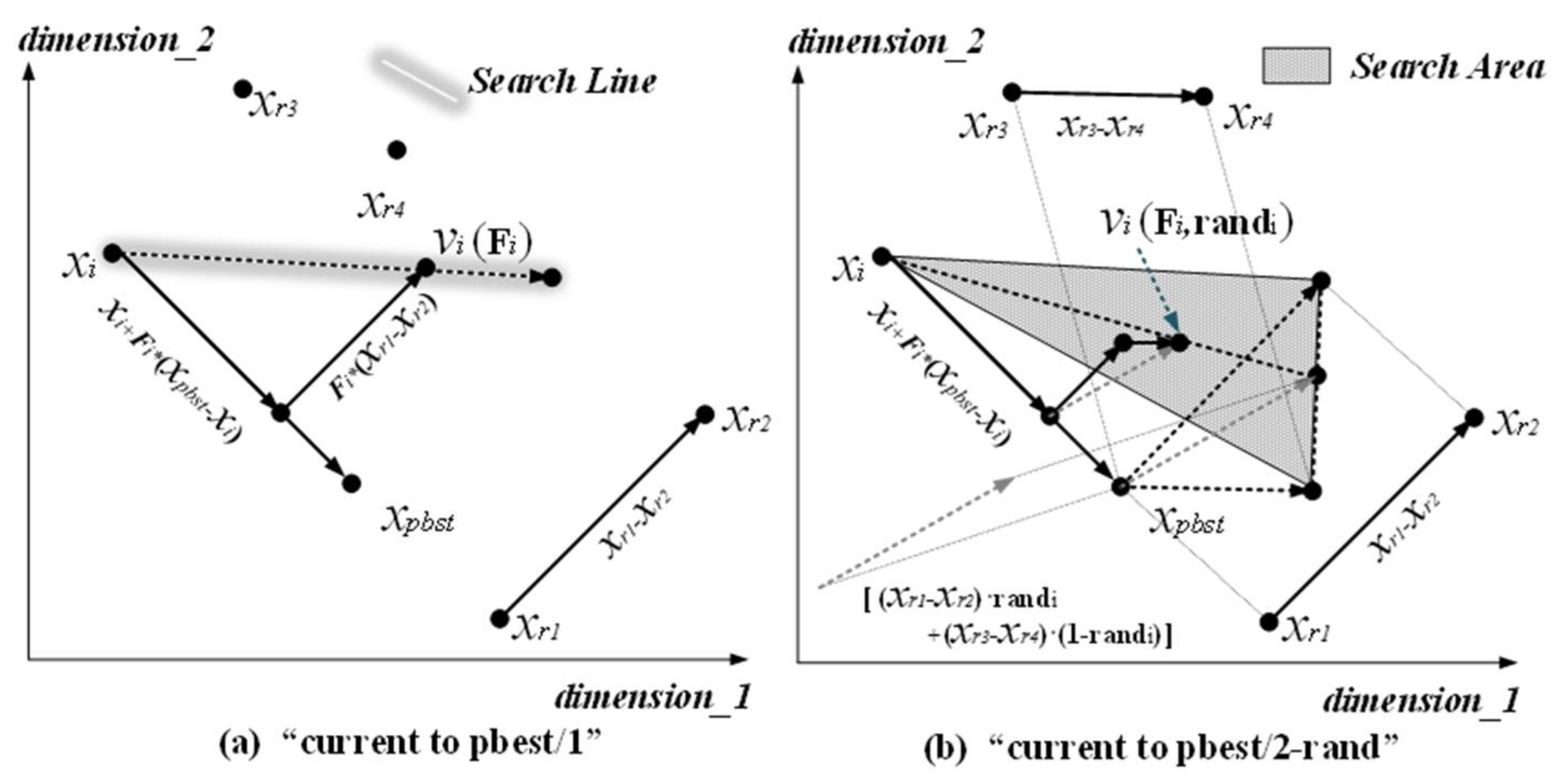
In Equation (16), the individual x p b e s t , G is randomly selected from the top N × p ( p [ 0 , 1 ] ) members in the G-th generation. “current to pbest/1” depends on the control parameter p to balance exploitation and exploration (small p behaves more greedily). x i , G and x r 1 , G are selected from P in the same way as in Equation (12), while x r 2 , G is randomly chosen from the union P A , of the current population and the archive. We present an improved mutation strategy “current to pbest/2-rand” to improve the search range based on mutation strategy “current to pbest/1”, which is expressed as follows:
v i , G = x i , G + F i ( x p b e s t , G x i , G ) + F i [ ( x r 1 , G x r 2 , G ) rand i + ( x r 3 , G x r 4 , G ) ( 1 rand i ) ]
where rand i is a uniformly distributed random number between [0,1]. x i , G , x r 1 , G and x r 3 , G are selected randomly and different within the range {1, NP} from P in the same way as in formula (16), while x r 2 , G and x r 4 , G is randomly chosen from the union, P A , of the current population and the archive. The two mutation strategies are illustrated in Figure 2.
As seen in Figure 2a, v i , G is the mutation individual generated for individual x i , G . According to the principle of vector addition, the position of v i , G changes with the associated mutation factor F i , and its position only exists on this “Search Line”. Mutation strategy “current to pbest/2-rand” uses rand i and linear combination of ( x r 1 , G x r 2 , G ) rand i + ( x r 3 , G x r 4 , G ) ( 1 rand i ) to expand the search range. By the varying value rand i , v i , G can search anywhere in the shaded triangle area with the change of the F i and rand i (see Figure 2b). Obviously, the search range of “current to pbest/2-rand” is much larger than that of “current to pbest/1”.

3.2.2. The PIRFE Strategy

The PIRFE strategy is proposed to avoid individuals in a local optimum lead useless evolution. When an individual falls into a local optimal, it is extremely difficult to produce an effective mutation to jump out of the local optimal. The individual failing evolution number (IFEN) is defined to record the number of individual failing evolution, and it is initialized to zero. x i , G generates u i , G through mutation and crossover. If x i , G + 1 produces a failing evolution and x i , G + 1 is better than u i , G + 1 , I F E N i , G + 1 is equal to I F E N i , G plus one, otherwise I F E N i , G + 1 will reset to zero. I F E N i , G + 1 is illustrated as follows:
I F E N i , G + 1 = { 0 if   u i , G + 1   is   better   than   x i , G + 1 I F E N i , G + 1 otherwise
If x i produces failing evolutions for I F E N i generations, and I F E N i is more than limit evolution generations (see formula (18)), x i falls into local optimal. The L E G represents the largest evolution generation allowing failure evolutions. In the next evolutionary process, we should avoid involving x i . x i should be replaced by a new individual randomly selected in population. The framework of the PIRFE strategy is as follows (Figure 3):

3.2.3. Control Parameters Assignments

SHADE maintains a historical memory with H entries for both DE control parameters C R , F , M C R and M F . The scaling factor F [ 0 ,   1 ] controls the magnitude of the differential mutation operator and C R [ 0 ,   1 ] is the crossover rate. In the beginning, the contents of M C R , k , M F , k ( k = 1 , , H ) are all initialized to 0.5. In each generation G, the control parameters C R i and F i used by each individual x i are generated by randomly selecting an index r i from [ 1 ,   H ] , and then applying the formulas (19) and (20):
C R i = { 0 if   M C R , r i = randn i ( M C R , r i , 0.1 ) otherwise
F i = randc i ( M F , r i , 0.1 )
In case a value for C R i outside of [0, 1] is generated, it is replaced by the limit value (0 or 1) closest to the generated value. When F i > 1, is truncated to 1, and when F i ≤ 0, formula (20) is repeatedly applied to generate a valid value. These manners are determined according to the procedure for JADE [38]. In formula (19), if M C R , r i has been assigned the “terminal value” ⊥, C R i is set to 0.
In each generation, in formula (17), C R i and F i values that succeed in generating a trial individual u i , G better than the parent individual x i , G are recorded as S C R , S F . At the end of the generation, the contents of memory are updated as follows:
M C R , k , G + 1 = { if   M C R , k , G =   or   max ( S C R ) = 0 mean W A ( S C R ) if   S C R M C R , k , G otherwise
M F , k , G + 1 = { mean W L ( S F ) if   S F M F , k , G otherwise
An index k (1 < k < H) determines the position in the memory to update. At the beginning of the search k is initialized to 1. k is incremented whenever a new element is inserted into the history. If > H, k is set to 1. In generation G, the k-th element in the memory is updated. In the update formula (21) and (22), when all individuals in generation G fail to generate an individual better than the parent, i.e., S C R = S F = , the memory is not updated. Also, the weighted mean m e a n W A ( S C R ) is computed according to formula (23) by Peng et al. [44]. The weighted Lehmer mean m e a n W L ( S F ) is computed using the formula below, and as with m e a n W A ( S C R ) :
m e a n W L ( S F ) = k | S F | w k S F , k 2 / k | S F | w k S F , k
m e a n W A ( S C R ) = k = 1 | S C R | w k S C R , k
w k = f k / k = 1 | S C R | f k
where f k = | f ( u i , G ) f ( x i , G ) | . In the same paper, they also proposed a restart strategy for JADE [38].
LSHADE put forward a new method of NP setting—LPSR which reduces the population linearly. The population size at generation 1 is N i n i t , and the population at the end of the run is N m i n . After each generation G, the population size in the next generation, N G + 1 is computed according to formula (26):
N G + 1 = round [ ( ( N m i n N i n i t ) / M A X N F E ) N F E + N i n i t ]
If N m i n is set to the smallest possible value, the evolutionary operators can be applied in the case of iLSHADE, N m i n = 6 because the mutation strategy “current to pbest/2-rand” showed as formula (17) requires 4 individuals. N F E is the current number of fitness evaluations, and M A X N F E is the maximum number of fitness evaluations. Whenever N G + 1 < N G , the ( N G N G + 1 ) worst-ranking individuals are deleted from the population. Similarly, the external archive size | A | is set to N i n i t multiplied by a parameter r a r c , | A | = round ( N i n i t × r a r c ) . In addition, external archive A is same as population, whenever | A | G + 1 < | A | G , the ( | A | G | A | G + 1 ) worst-ranking individuals are deleted from the A . The p value for “current to pbest/2-rand” in each generation G is computed as follows:
p = ( p m a x p m i n ) rand ( 0 , 1 ) + p m i n
where rand ( 0 , 1 ) returns a uniformly distributed random number in [ 0 , 1 ] , p is a random value in [ p m a x , p m i n ] . Finally, the pseudo-code of the iLSHADE algorithm is given in Figure 4.

4. Numerical Experiment

The iLSHADE algorithm was tested in both low and high dimension on a set of 10 benchmark functions demonstrated in Table 1. Table 1 indicates benchmark problems with different structures and characteristics. In the table, ‘‘O-V’’ means the optimum fitness and “O-S” stands for the optimum solution. f1, f2, f3, f5 and f6 are unimodal optimization problems to evaluate the convergence, while f4, f7, f8,f9 and f10 are multimodal optimization problems with a huge number of local optima to test the convergence precision [18].
The iLSHADE is compared to DE and other improved DE like LSHADE, JADE, CoDE and jDE. The number of function evaluations is used to appraise the convergence. These experiments are made on a personal computer, Windows10, Intel(R) Core(TM) i7-5500U CPU@ 2.40GHZ, RAM 8.00 GB. The dimension of benchmark functions is D = 10 in low dimension and 30 in high dimension, and 51 runs of an algorithm were needed for each function. The maximum number of objective function evaluations is D × 10,000. The optimal values are known for all benchmark functions.
In the experiments, the parameters in LSHADE, JADE, CoDE, jDE and DE were kept unchanged refer to [33,36,38,39,42], and the parameter setting in the iLSHADE is same as LSHADE except the following parameters:
  • Using “current to pbest/2-rand” mutation strategy,
  • The p value for mutation strategy is computed as p G = rand [ p min , p max ] , where p min = 2 / N P is set such that when x p b e s t , G is selected, at least 2 individuals are needed, and p max = 0.25 .
  • Initial population size N i n i t = 15 l o g ( D ) D , the control parameter of external archive size r a r c = 2 .
  • Historical memory size H = 6; set a final pair of parameters M F [ H ] = 0.2 and M C R [ H ] = 0.8 , other M F values are initialized to 0.5 and other M C R are initialized to 0.8.
  • PIRFE parameter L E G = 50.
The aggregate results of statistical testing ( + , , ) on 10 functions are shown in Table 2 and Table 3. The symbols + , , indicate that a given algorithm performed significantly better ( + ), significantly worse ( ), or not significantly different better or worse ( ) compared to iLSHADE using the Wilcoxon rank-sum test [45] (significantly, p < 0.05).
1. Simulation in low dimension.
Table 2 summarizes the experimental results in low dimension. It shows that iLSHADE eventually converges to optimum for 8 test functions except f 2 and f 9 . Moreover, iLSHADE significantly outperforms JADE, CoDE, jDE, DE. Compared to LSHADE, iLSHADE beats LSHADE on two test functions f 2 and f 3 . Especially in f 3 , only iLSHADE converges to the global optimal value. Overall, iLSHADE performs better than other algorithms on low dimension optimization problems.
2. Simulation in high dimension.
The experimental results in high dimension are summarized in Table 3. iLSHADE eventually converges to optimum for 7 test functions except f 2 , f 8 and f 9 . iLSHADE performs the best in f 2 and f 9 , although it does not converge to the global optimal. While on f 8 , JADE performs the best. The proposed algorithm is not good as expected. Above all, iLSHADE has an obvious advantage over other algorithms on high dimension optimization problems.
To sum up, iLSHADE is suitable for both low dimension and high dimension, meaning that the improvement proposed in this paper is effective.

5. Implementation of iLSHADE for LSLCHS

5.1. Solution Structure and Initial Population

To handle constraints and calculate objective function, solution structure for the LSLCHS comprises a group of monthly water levels as the decision variables shown as follows.
X = [ X 1 X 2 X M ] = [ x 1 1 , x 2 1 , x T 1 x 1 2 , x 2 2 , x T 2 x 1 M , x 2 M , x T M ]
where M is the number of hydropower stations, T (12 month in a year) is the number of intervals. In algorithms relying on heuristic search, initial population is an important issue to convergence speed and population diversity. The iLSHADE has a large initial population size based on LPSR and ensures the diversity of the population by random initialization.

5.2. Constraint Handling

It is multiple and complicate for flow constraint, power generating constraint, amplitude of water level variation and hydraulic connection of cascade. The handling measure currently used for water balance constraint, water level constraint and boundary condition is often corrected to the boundary [18,46]. It has defects such as: (1) The direction of the entering feasible domain is relatively simple and centered on the boundary because of the excessive attention to the rapid into the feasible area; (2) When there are multiple feasible domains, it is easy to ignore small feasible areas;
The ε-constrained method is first proposed by Takahama et al. [47], which relaxes the greed of the feasibility criterion to the constraint conditions. The ε value is set as threshold value in ε-constrained method. In general, constrained optimization maximum problems can be mathematically formulated as follows:
max   f ( x ) ,   x = ( x 1 , , x D )
subject   to   { g i ( x ) 0    i = 1 , 2 , , m h j ( x ) = 0    j = 1 , 2 , , n
where g i ( x ) is inequality constraints, m is the total number of inequality constraint. h j ( x ) is equality constraints and n is the total number of equality constraints. The value of constraint violation φ ( x ) can be calculated in the following formula (30), and φ ( x ) of infeasible solutions is bigger than 0.
φ ( x ) = i = 0 m max ( 0 , g i ( x ) ) + j = 1 n ( | h j ( x ) | , 0 )
When the constraint violation values of both solutions are smaller than ε value, the one with better objective function value is selected. Otherwise, the one with smaller constraint violation value is selected. Overall, when any of the following conditions are met, x i is superior to x j :
{ f ( x i ) < f ( x j ) ,   if   g ( x i ) ε g ( x j ) ε f ( x i ) < f ( x j ) ,   if   g ( x i ) = g ( x j ) g ( x i ) < g ( x j ) ,   otherwise
and the final effectiveness of e-constrained method strongly depends on the control method of ε value. Takahama et al. [47] proposed the following method,
ε ( 0 ) = φ ( P 0 θ )
ε ( t ) = { ε ( 0 ) ( 1 t / T c ) c p 0 < t < T c 0 t > T c
where P 0 θ is the top θ -th individual in the initial population, c p is a control parameter. If the number of iterations t is less than a given threshold value T c , the ε value declines in an exponential way. Otherwise, ε is set to 0 (see formula (33) and (34)).
The ε-constrained method can expand search space, avoid the constraint correction for unfeasible solutions and enable to search infeasible region that is around feasible region. However, the constraints consist of flow, power generating and amplitude of water level. Operating water level in LSLCHS problem is multiple and complex. Their units are not integrated, and the physical quantities corresponding to the same level of different reservoirs are different. To solve the above problems, we proposed ε -constrained in cascade reservoir operation method ( ε -CRO) with unify different physical quantities constraint violation. The ε -CRO chooses water to unify different physical quantities constraint violation because all constraints can be converted to outflow constraint and flow accumulated over time as water. The feasible range of outflow Q i , t is expressed in formula (35) and (36).
Q ¯ i , t + 1 = min { Q i , t + 1 max ( V ( Z i , t ) V ( Z i , t + 1 min ) ) / Δ t ( V ( Z i , t ) V ( Z i , t Δ Z i ) ) / Δ t
Q _ i , t + 1 = max { Q i , t + 1 min I i , t + ( V ( Z i , t ) V ( Z i , t + 1 max ) ) / Δ t I i , t + ( V ( Z i , t ) V ( Z i , t + Δ Z i ) ) / Δ t Q i , t + 1 min   N
where Z i , t represents the i-th reservoir water level at the -th period, Z ( V ) is the relationship between water level and storage. Q ¯ i , t + 1 and Q _ i , t + 1 stand for the minimum and maximum outflow under all constraints. Q i , t + 1 min   N is the outflow for guaranteed output and Δ t stands for time horizon. The value of constraint violation in LSLCHS problem φ C R O ( x ) can be calculated as follows:
φ C R O ( x ) = i = 1 M t = 1 T [ max ( 0 , Q i , t Q ¯ i , t + 1 ) + max ( 0 , Q _ i , t + 1 Q i , t ) ]
ε C R O ( 0 ) and ε C R O ( t ) are calculated like in [47] except θ = 0.5, c p = 1 and T c = 0.5 * M A X N F E .

6. Case Study

6.1. Description of Case Study

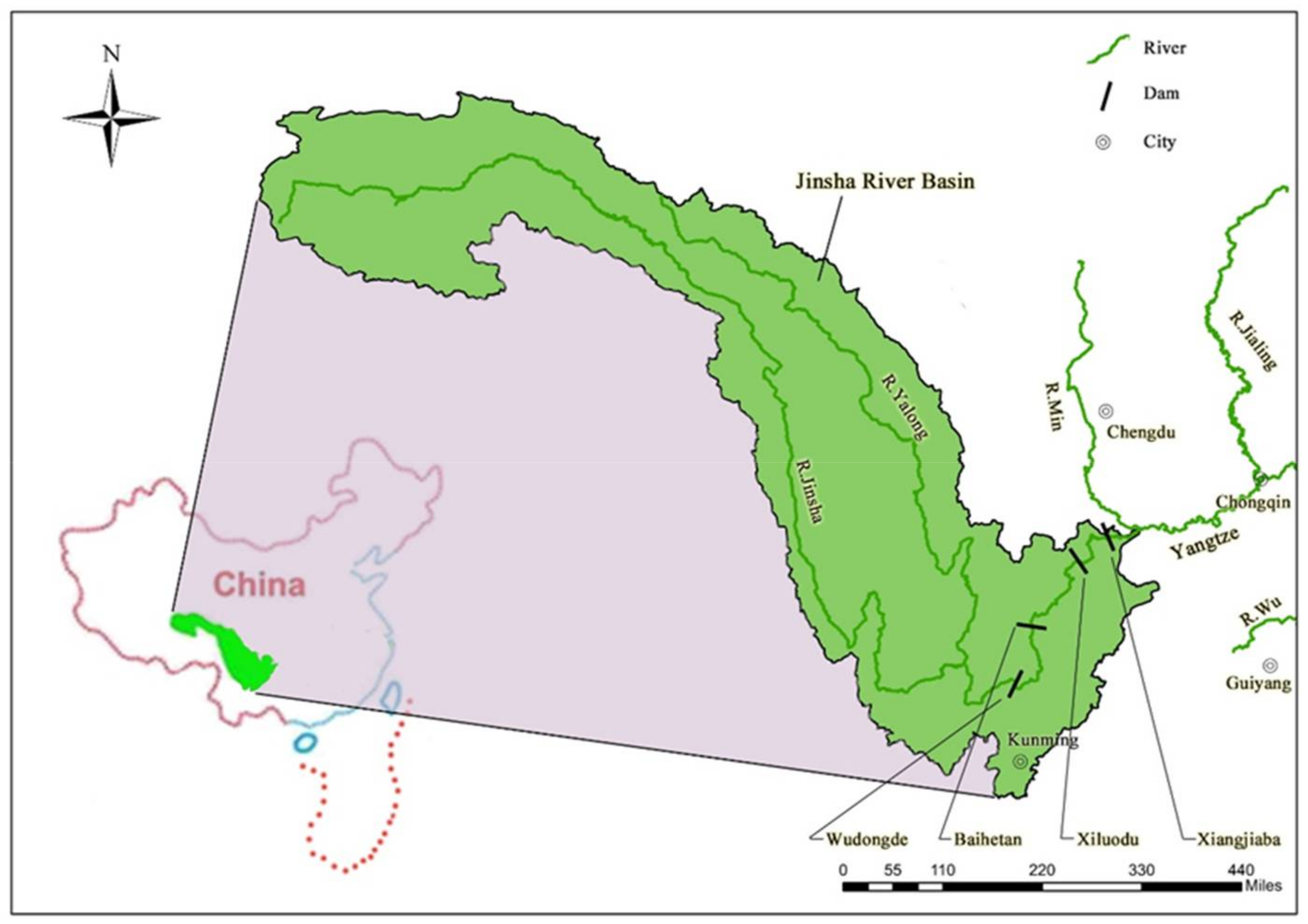
The Jinsha River, the upper stretch of the Yangtze River, is 2290 km long with a 485,000 km2 basin area flowing through the provinces of Qinghai, Sichuan, and Yunnan in western China (See in Figure 5). Along the river, there are four large hydropower stations with large installed capacity, huge regulating storage and high water head. The total installed capacity of the four large hydropower stations is twice more than the Three Gorges Project (the largest hydropower station in the world). The main parameters of these hydropower stations are listed in Table 4.

6.2. Results and Analysis

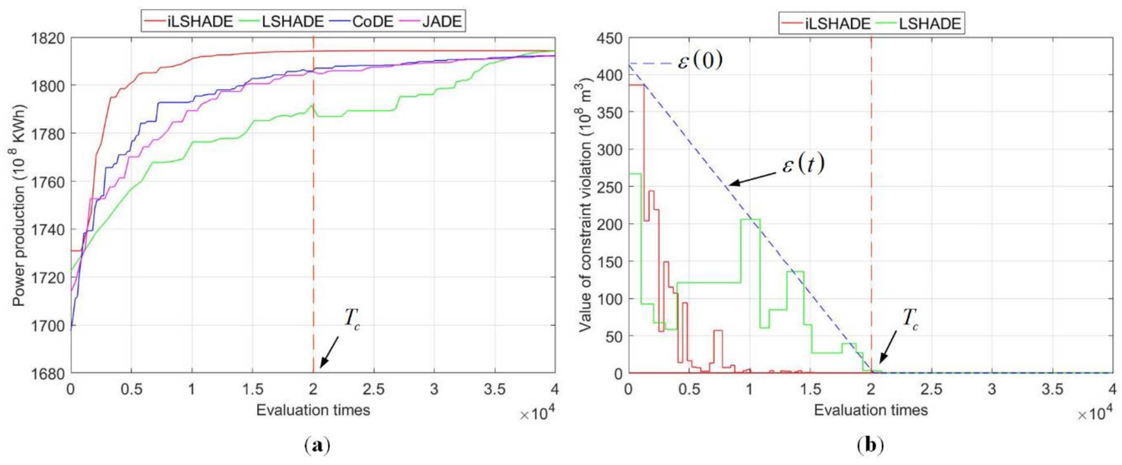
In the case, the four large hydropower stations are all taken into consideration. According to historical runoff from 1959 to 2014 in the basin, three typical years are chosen to be the inflow conditions: wet year (historical runoff of 1999), normal year (2008) and dry year (1969). Simulation results of iLSHADE are compared to LSHADE, JADE and CoDE in three typical years. The initial water level and terminal water level of all the hydropower stations are set to the normal water level. The schedule period consists of 12 intervals with one month for each interval. In addition, the parameters in all algorithms are the same as those mentioned in Section 4. The maximum evaluation time is set to 40,000.
Table 5 represents that iLSHADE gains the best benefit of power production in three typical years. The convergence process of different algorithms in dry year is shown in Figure 6. Compared to LSHADE, JADE and CoDE on average optimal benefit of 51 independent simulations are illustrated in Table 5, iLSHADE increases the power production by 2.02, 4.04, 2.39 (108 KWh) in wet year, 3.03, 7.37, 3.76 (108 KWh) in normal year, 3.48, 5.68, 1.96 (108 KWh) in dry year. Obviously, the proposed iLSHADE is superior when solving LSLCHS problem by obtaining the maximal benefit of power production efficiently. In particular, the standard deviation of 51 independent simulations in iLSHADE is 0.02 in wet year, 0.01 in normal year, 0.01 in dry year, which shows that the convergence stability of iLSHADE is better than other algorithms. Meanwhile, it can be seen easily from Figure 6a that iLSHADE can avoid premature convergence effectively, at the same evaluation times keep a fast convergence speed compared to LSHADE, CoDE and JADE. Figure 6b depicts that the φ C R O ( x ) of iLSHADE and LSHADE frequent changes and always lower than ε C R O ( t ) , until evaluation times is greater than T c , φ C R O ( x ) is limited to 0.
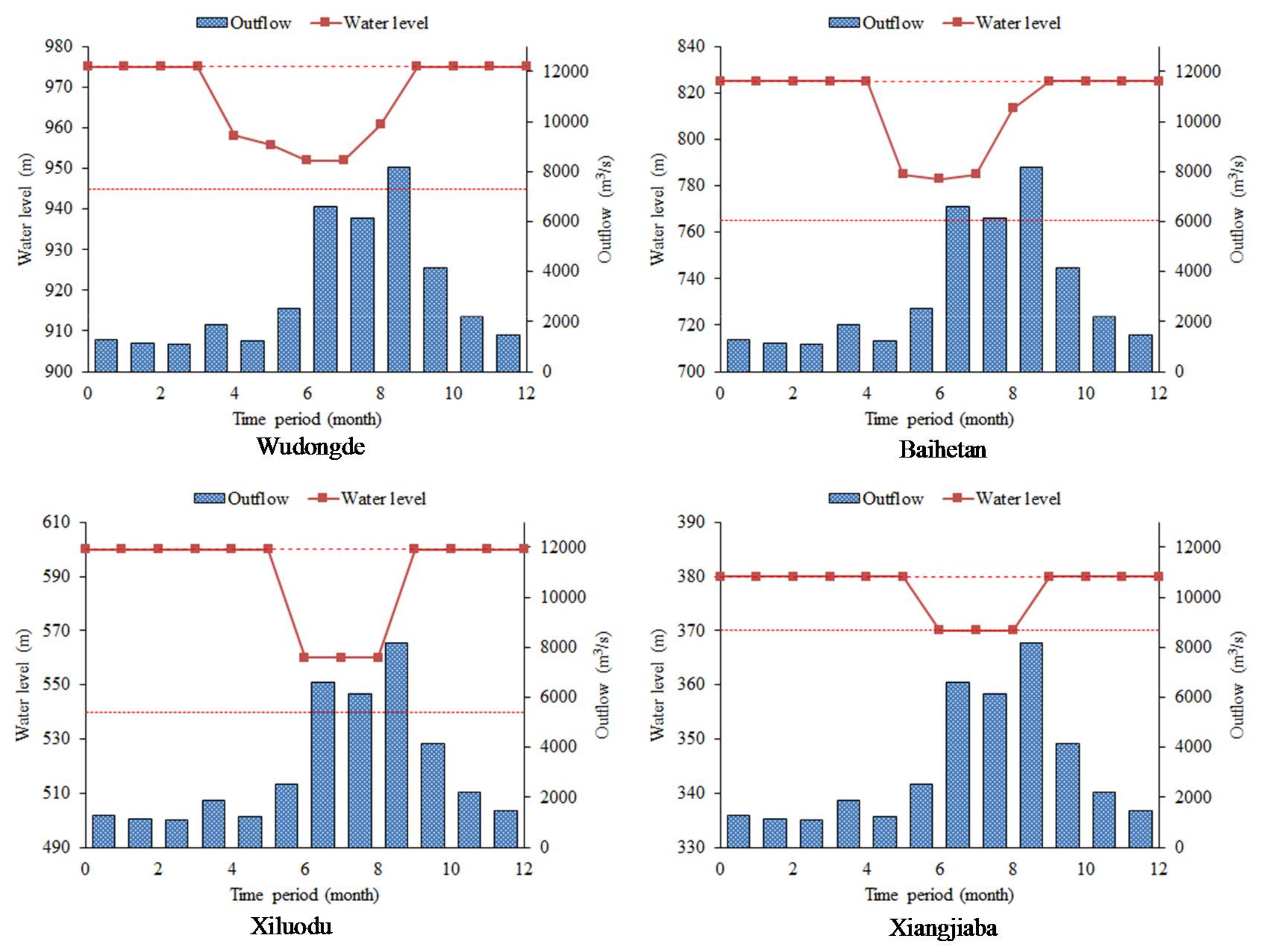
The monthly reservoir water levels and outflow, as well as the optimal schedule result of Wudongde, Baihetan, Xiluodu and Xiangjiaba result in normal year obtained by iLSHADE are shown in Figure 7. Due to sufficient inflow, the cascade reservoir does not need to release storage capacity to meet the constraints of minimum outflow limit during the dry season from January to March. The inflow of Wudongde is very low in April, so the cascade reservoir needs to release storage capacity to meet the constraint requirements. As one of the upstream reservoirs, Wudongde first lowers the water level. To reduce the water spillage before flood season, Baihetan will lower its water level below the flood control level in advance and impound some water at the last period. Xiluodu and Xiangjiaba lower the water level in the last period. During the impoundment period, Wudongde and Baihetan store water to normal water level before Xiluodu and Xiangjiaba in October. In this way, the water in upstream reservoirs can utilize the downstream high hydraulic head to generate more electric power.
Furthermore, the historical runoff data from 1959 to 2014 are selected for long sequence calculation. The parameters in all algorithms are the same as those mentioned in Section 6.2 and the maximum evaluation time is set to 40,000. The average adding annual power production that iLSHADE compares to LSHADE, JADE and CoDE is presented in Figure 8. It can be seen clearly from Figure 8 that iLSHADE is superior compared to other algorithm in solving the LSLCHS problem with different types of historical runoff from 1959 to 2014.
According to the above analysis, proposed iLSHADE is superior when solving LSLCHS problem in different types of runoff by obtaining the maximize benefit of electric power production. All these experiment results fully demonstrate that iLSHADE is a competitive method to solve the LSLCHS problem.

7. Conclusions

An iLSHADE algorithm with new mutation strategy “current to pbest/2-rand” and PIRFE strategy has been developed in this paper to solve the LSLCHS problem. The significant modifications are mainly focused on preventing premature convergence and accelerating convergence. To verify the performance of iLSHADE, numerical simulation in both low and high dimension on a set of 10 benchmark functions has been done. Compared with other improved differential evolution algorithms, iLSHADE obtains better performance with all ten functions in the low dimension and nine functions in the high dimension. This indicates that the proposed new mutation strategy “current to pbest/2-rand” and PIRFE strategy in iLSHADE enhance the performance of original algorithm LSHADE effectively. Then iLSHADE is applied to solve LSLCHS problem for four large hydropower stations in Jinsha River. Compared to LSHADE, JADE and CoDE on average optimal benefit, iLSHADE increases the power production by 3.03, 7.37, 3.76 (108 KWh) in a normal year. In particular, the standard deviation of 51 independent simulations in iLSHADE is far lower than other algorithms. Moreover, according to its successful simulation performance with the historical runoff data from 1959 to 2014, iLSHADE can obtain better schedule results with lager generation benefits and better convergence property compared to LSHADE, JADE and CoDE. Above all, iLSHADE is a valid and reliable tool in solving the LSLCHS problem. Future research should consider the iLSHADE algorithm combined with other methods when solving multi objective scheduling problems in LSLCHS problem.

Acknowledgments

This work is supported by the National Natural Science Foundation Key Project of China (No. 91547208), the National Natural Science Foundation of China (No. 51579107), the National Key R&D Program of China (No. 2016YFC0402205) and the Foundation of Huazhong University of Science and Technology (No. 2017KFYXJJ209). Special thanks are given to the anonymous reviewers and editors for their constructive comments.

Author Contributions

Xiaohao Wen and Zhongzheng He designed and conducted the experiments. Xiaohao Wen wrote the draft of the paper. Zhongzheng He prepared the figures for this paper. Jianzhong Zhou proposed the main structure of this study. Chao Wang provided useful advice and made some corrections. All authors read and approved the final manuscript.

Conflicts of Interest

The authors declare no conflict of interest.

References

  1. Lior, N. Sustainable energy development: The present (2011) situation and possible paths to the future. Energy 2012, 43, 174–191. [Google Scholar] [CrossRef]
  2. Wu, X.-Y.; Cheng, C.-T.; Shen, J.-J.; Luo, B.; Liao, S.-L.; Li, G. A multi-objective short term hydropower scheduling model for peak shaving. Int. J. Electr. Power Energy Syst. 2015, 68, 278–293. [Google Scholar] [CrossRef]
  3. Madani, K. Hydropower licensing and climate change: Insights from cooperative game theory. Adv. Water Resour. 2011, 34, 174–183. [Google Scholar] [CrossRef]
  4. Xu, J.; Ni, T.; Zheng, B. Hydropower development trends from a technological paradigm perspective. Energy Convers. Manag. 2015, 90, 195–206. [Google Scholar] [CrossRef]
  5. Chang, X.; Liu, X.; Zhou, W. Hydropower in china at present and its further development. Energy 2010, 35, 4400–4406. [Google Scholar] [CrossRef]
  6. Tasdemiroglu, E. Development of small hydropower in Türkiye. Energy 1993, 18, 699–702. [Google Scholar] [CrossRef]
  7. Zhou, Y.; Guo, S.; Xu, C.-Y.; Liu, P.; Qin, H. Deriving joint optimal refill rules for cascade reservoirs with multi-objective evaluation. J. Hydrol. 2015, 524, 166–181. [Google Scholar] [CrossRef]
  8. Jiang, Z.; Li, A.; Ji, C.; Qin, H.; Yu, S.; Li, Y. Research and application of key technologies in drawing energy storage operation chart by discriminant coefficient method. Energy 2016, 114, 774–786. [Google Scholar] [CrossRef]
  9. Chen, L.; Singh, V.P. Entropy-based derivation of generalized distributions for hydrometeorological frequency analysis. J. Hydrol. 2017. [Google Scholar] [CrossRef]
  10. Chen, L.; Singh, V.P.; Huang, K. Bayesian technique for the selection of probability distributions for frequency analyses of hydrometeorological extremes. Entropy 2018, 20, 117. [Google Scholar] [CrossRef]
  11. Chen, L.; Singh, V.P.; Guo, S.; Zhou, J.; Zhang, J.; Liu, P. An objective method for partitioning the entire flood season into multiple sub-seasons. J. Hydrol. 2015, 528, 621–630. [Google Scholar] [CrossRef]
  12. Chen, L.; Singh, V.P.; Lu, W.; Zhang, J.; Zhou, J.; Guo, S. Streamflow forecast uncertainty evolution and its effect on real-time reservoir operation. J. Hydrol. 2016, 540, 712–726. [Google Scholar] [CrossRef]
  13. Djebou, D.C.S. Spectrum of climate change and streamflow alteration at a watershed scale. Environ. Earth Sci. 2017, 76, 653. [Google Scholar] [CrossRef]
  14. Sohoulande Djebou, D.C.; Singh, V.P. Entropy-based index for spatiotemporal analysis of streamflow, precipitation, and land-cover. J. Hydrol. Eng. 2016, 21, 05016024. [Google Scholar] [CrossRef]
  15. Xu, B.; Zhong, P.-A.; Wu, Y.; Fu, F.; Chen, Y.; Zhao, Y. A multiobjective stochastic programming model for hydropower hedging operations under inexact information. Water Resour. Manag. 2017, 31, 4649–4667. [Google Scholar] [CrossRef]
  16. Mahmoud, M.; Dutton, K.; Denman, M. Dynamical modelling and simulation of a cascaded reserevoirs hydropower plant. Electr. Power Syst. Res. 2004, 70, 129–139. [Google Scholar] [CrossRef]
  17. Cârdu, M.; Bara, T. Romanian achievement in hydro-power plants. Energy Convers. Manag. 1998, 39, 1193–1201. [Google Scholar] [CrossRef]
  18. Wang, C.; Zhou, J.; Lu, P.; Yuan, L. Long-term scheduling of large cascade hydropower stations in Jinsha river, China. Energy Convers. Manag. 2015, 90, 476–487. [Google Scholar] [CrossRef]
  19. Windsor, J.S. Optimization model for the operation of flood control systems. Water Resour. Res. 1973, 9, 1219–1226. [Google Scholar] [CrossRef]
  20. Yoo, J.-H. Maximization of hydropower generation through the application of a linear programming model. J. Hydrol. 2009, 376, 182–187. [Google Scholar] [CrossRef]
  21. Brandao, J.L.B. Performance of the equivalent reservoir modelling technique for multi-reservoir hydropower systems. Water Resour. Manag. 2010, 24, 3101–3114. [Google Scholar] [CrossRef]
  22. Catalão, J.P.D.S.; Pousinho, H.M.I.; Mendes, V.M.F. Scheduling of head-dependent cascaded hydro systems: Mixed-integer quadratic programming approach. Energy Convers. Manag. 2010, 51, 524–530. [Google Scholar] [CrossRef]
  23. Jiang, Z.; Qin, H.; Ji, C.; Feng, Z.; Zhou, J. Two dimension reduction methods for multi-dimensional dynamic programming and its application in cascade reservoirs operation optimization. Water 2017, 9, 634. [Google Scholar] [CrossRef]
  24. Lee, J.H.; Labadie, J.W. Stochastic optimization of multireservoir systems via reinforcement learning. Water Resour. Res. 2007, 43. [Google Scholar] [CrossRef]
  25. Nanda, J.; Bijwe, P.R. Optimal hydrothermal scheduling with cascaded plants using progressive optimality algorithm. IEEE Trans. Power Appar. Syst. 1981, PAS-100, 2093–2099. [Google Scholar] [CrossRef]
  26. Jiang, Z.; Ji, C.; Qin, H.; Feng, Z. Multi-stage progressive optimality algorithm and its application in energy storage operation chart optimization of cascade reservoirs. Energy 2018, 148, 309–323. [Google Scholar] [CrossRef]
  27. Jiang, C.; Bompard, E. A self-adaptive chaotic particle swarm algorithm for short term hydroelectric system scheduling in deregulated environment. Energy Convers. Manag. 2005, 46, 2689–2696. [Google Scholar]
  28. Cheng, C.T.; Liao, S.L.; Tang, Z.T.; Zhao, M.Y. Comparison of particle swarm optimization and dynamic programming for large scale hydro unit load dispatch. Energy Convers. Manag. 2009, 50, 3007–3014. [Google Scholar] [CrossRef]
  29. Hınçal, O.; Altan-Sakarya, A.B.; Ger, A.M. Optimization of multireservoir systems by genetic algorithm. Water Resour. Manag. 2011, 25, 1465–1487. [Google Scholar] [CrossRef]
  30. Yuan, X.; Yuan, Y. Application of cultural algorithm to generation scheduling of hydrothermal systems. Energy Convers. Manag. 2006, 47, 2192–2201. [Google Scholar] [CrossRef]
  31. Wang, W.; Li, C.; Liao, X.; Qin, H. Study on unit commitment problem considering pumped storage and renewable energy via a novel binary artificial sheep algorithm. Appl. Energy 2017, 187, 612–626. [Google Scholar] [CrossRef]
  32. Jalali, M.R.; Afshar, A.; Mariño, M.A. Multi-colony ant algorithm for continuous multi-reservoir operation optimization problem. Water Resour. Manag. 2007, 21, 1429–1447. [Google Scholar] [CrossRef]
  33. Storn, R.; Price, K. Differential evolution—A simple and efficient heuristic for global optimization over continuous spaces. J. Glob. Optim. 1997, 11, 341–359. [Google Scholar] [CrossRef]
  34. Lu, Y.; Zhou, J.; Qin, H.; Li, Y.; Zhang, Y. An adaptive hybrid differential evolution algorithm for dynamic economic dispatch with valve-point effects. Expert Syst. Appl. Int. J. 2010, 37, 4842–4849. [Google Scholar] [CrossRef]
  35. Yuan, X.; Cao, B.; Yang, B.; Yuan, Y. Hydrothermal scheduling using chaotic hybrid differential evolution. Energy Convers. Manag. 2008, 49, 3627–3633. [Google Scholar] [CrossRef]
  36. Brest, J.; Greiner, S.; Boskovic, B.; Mernik, M.; Zumer, V. Self-adapting control parameters in differential evolution: A comparative study on numerical benchmark problems. IEEE Trans. Evolut. Comput. 2006, 10, 646–657. [Google Scholar] [CrossRef]
  37. Qin, A.K.; Huang, V.L.; Suganthan, P.N. Differential evolution algorithm with strategy adaptation for global numerical optimization. IEEE Trans. Evolut. Comput. 2009, 13, 398–417. [Google Scholar] [CrossRef]
  38. Zhang, J.; Sanderson, A.C. Jade: Adaptive differential evolution with optional external archive. IEEE Trans. Evolut. Comput. 2009, 13, 945–958. [Google Scholar] [CrossRef]
  39. Wang, Y.; Cai, Z.; Zhang, Q. Differential evolution with composite trial vector generation strategies and control parameters. IEEE Trans. Evolut. Comput. 2011, 15, 55–66. [Google Scholar] [CrossRef]
  40. Mallipeddi, R.; Suganthan, P.N.; Pan, Q.K.; Tasgetiren, M.F. Differential evolution algorithm with ensemble of parameters and mutation strategies. Appl. Soft Comput. 2011, 11, 1679–1696. [Google Scholar] [CrossRef]
  41. Tanabe, R.; Fukunaga, A. Success-History Based Parameter Adaptation for Differential Evolution. In Proceedings of the 2013 IEEE Congress on Evolutionary Computation, Cancun, Mexico, 20–23 June 2013; pp. 71–78. [Google Scholar]
  42. Tanabe, R.; Fukunaga, A.S. Improving the search performance of shade using linear population size reduction. In Proceedings of the 2014 IEEE Congress on Evolutionary Computation, Beijing, China, 6–11 July 2014; pp. 1658–1665. [Google Scholar]
  43. Liang, J.J.; Qu, B.Y.; Suganthan, P.N. Problem Definitions and Evaluation Criteria for the CEC 2014 Special Session and Competition on Single Objective Real-Parameter Numerical Optimization; Computational Intelligence Laboratory, Zhengzhou University, Zhengzhou China and Technical Report; Nanyang Technological University: Singapore, 2013. [Google Scholar]
  44. Peng, F.; Tang, K.; Chen, G.; Yao, X. Multi-start jade with knowledge transfer for numerical optimization. In Proceedings of the Eleventh Conference on Congress on Evolutionary Computation, Trondheim, Norway, 18–21 May 2009; pp. 1889–1895. [Google Scholar]
  45. Cortina-Borja, M. Handbook of Parametric and Nonparametric Statistical Procedures, 5th ed.; Sheskin, J., Ed.; CRC Press: Boca Raton, FL, USA, 2012; p. 382. [Google Scholar]
  46. Liao, X.; Zhou, J.; Zhang, R.; Zhang, Y. An adaptive artificial bee colony algorithm for long-term economic dispatch in cascaded hydropower systems. Int. J. Electr. Power Energy Syst. 2012, 43, 1340–1345. [Google Scholar] [CrossRef]
  47. Takahama, T.; Sakai, S.; Iwane, N. Constrained optimization by the ε constrained hybrid algorithm of particle swarm optimization and genetic algorithm. In Proceedings of the Australasian Joint Conference on Artificial Intelligence, Sydney, Australia, 5–9 December 2005; pp. 389–400. [Google Scholar]
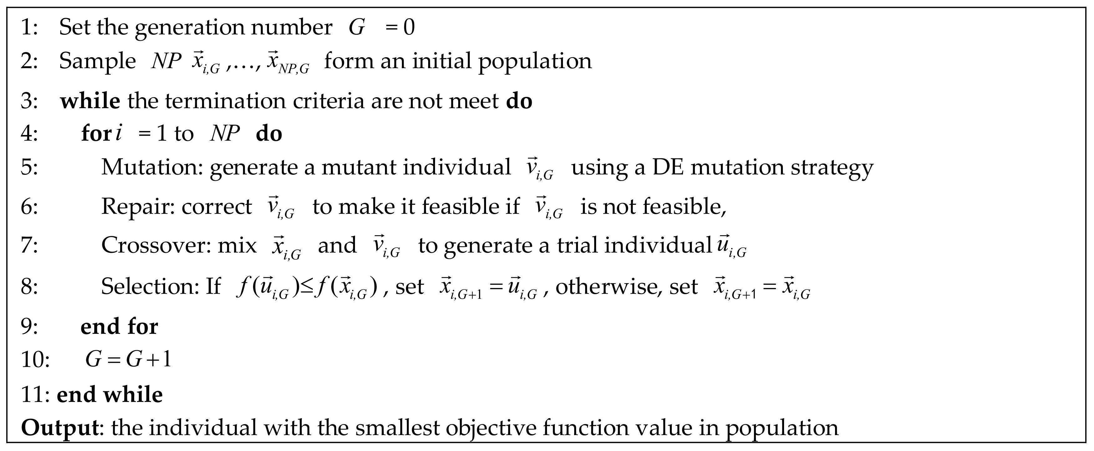
Figure 1. Pseudocode of DE.
Water 10 00383 g001
Figure 2. Illustration of the DE mutation strategy in two dimensions.
Water 10 00383 g002
Figure 3. Pseudocode of PIRFE strategy.
Water 10 00383 g003
Figure 4. Pseudocode of iLSHADE.
Water 10 00383 g004
Figure 5. The location of the Jinsha River Basin in China.
Water 10 00383 g005
Figure 6. Convergence process of different algorithms.
Water 10 00383 g006
Figure 7. Optimal results in normal year by month.
Water 10 00383 g007
Figure 8. Historical runoff data from 1959 to 2014 for the annual power production increase that iLSHADE compares to LSHADE, JADE and CoDE.
Water 10 00383 g008
Table 1. Details of benchmark problems.
Benchmark FunctionNameDomainO-VO-S
f 1 = i = 1 n x i 2 Sphere [ 100 , 100 ] n 0 { 0 , 0 , , 0 }
f 2 = i = 1 n | x i | + i n | x i | Schwefel (2.2) [ 100 , 100 ] n 0 { 0 , 0 , , 0 }
f 3 = i = 1 n ( j = 1 i x j ) 2 Schwefel (1.2) [ 100 , 100 ] n 0 { 0 , 0 , , 0 }
f 4 = i = 1 n 1 [ 100 ( x i + 1 x i 2 ) 2 + ( x i 1 ) 2 ] Rosenbrock [ 30 , 30 ] n 0 { 0 , 0 , , 0 }
f 5 = i = 1 n ( x j + 0.5 ) 2 Step [ 100 , 100 ] n 0 { 0 , 0 , , 0 }
f 6 = i = 1 n i x i 4 Quartic [ 1.28 , 1.28 ] n 0 { 0 , 0 , , 0 }
f 7 = i = 1 n x i sin ( | x i | ) Schwefel (2.26) [ 500 , 500 ] n −418.9n*
f 8 = i = 1 n [ x i 2 10 cos ( 2 π x i ) + 10 ] Rastrigin [ 5.12 , 5.12 ] n 0 { 0 , 0 , , 0 }
f 9 = 20 exp ( 0.2 1 / n i = 1 n x i 2 ) exp ( 1 / n cos ( 2 π x i ) ) + 20 + e Ackley [ 32 , 32 ] n 0 { 0 , 0 , , 0 }
f 10 = 1 + i = 1 n x i 2 4000 + i n cos ( x i i ) Griewank [ 600 , 600 ] n 0 { 0 , 0 , , 0 }
Note: * (420.9876, 420.9876, …, 420.9876).
Table 2. Experimental results of 10 test functions in low dimension.
f LSHADE
Mean
(Std Dev)
JADE
Mean
(Std Dev)
CoDE
Mean
(Std Dev)
jDE
Mean
(Std Dev)
DE
Mean
(Std Dev)
iLSHADE
Mean
(Std Dev)
f 1 0.00 × 100
(0.00 × 100) ≈
8.61 × 10−36
(7.18 × 10−36) −
5.93 × 10−38
(7.34 × 10−38) −
1.15 × 10−38
(1.18 × 10−38) −
2.73 × 10−46
(1.42 × 10−45) −
0.00 × 100
(0.00 × 100)
f 2 6.49 × 10−49
(4.38 × 10−48) −
8.75 × 10⁻²⁰
(4.68 × 10⁻²⁰) −
7.88 × 10⁻²²
(6.58 × 10⁻²²) −
1.38 × 10⁻²²
(1.01 × 10⁻²²) −
8.03 × 10⁻²⁵
(1.65 × 10⁻²⁴) −
3.36 × 10−64
(2.05 × 10−63)
f 3 1.10 × 10−91
(5.90 × 10−91) −
2.81 × 10⁻³⁵
(2.75 × 10⁻³⁵) −
2.43 × 10−39
(4.02 × 10−39) −
1.24 × 10−40
(1.79 × 10−40) −
4.58 × 10−45
(2.03 × 10−44) −
0.00 × 100
(0.00 × 100)
f 4 0.00 × 100
(0.00 × 100) ≈
0.00 × 100
(0.00 × 100) ≈
1.47 × 10−05
(1.96 × 10−05) −
7.39 × 10−03
(9.11 × 10−03) −
7.82 × 10−02
(5.53 × 10−01) −
0.00 × 100
(0.00 × 100)
f 5 0.00 × 100
(0.00 × 100) ≈
0.00 × 100
(0.00 × 100) ≈
0.00 × 100
(0.00 × 100) ≈
0.00 × 100
(0.00 × 100) ≈
0.00 × 100
(0.00 × 100)≈
0.00 × 100
(0.00 × 100)
f 6 0.00 × 100
(0.00 × 100) ≈
1.40 × 10−71
(3.27 × 10−71) −
6.47 × 10−71
(1.52 × 10−70) −
1.40 × 10−72
(3.66 × 10−72) −
8.39 × 10−88
(4.17 × 10−87) −
0.00 × 100
(0.00 × 100)
f 7 −4189.83
(2.73 × 10⁻¹²) ≈
−4189.83
(2.73 × 10⁻¹²) ≈
−4189.83
(2.73 × 10⁻¹²) ≈
−4189.83
(2.73 × 10⁻¹²) ≈
−4189.83
(2.73 × 10⁻¹²) ≈
−4189.83
(2.73 × 10⁻¹²)
f 8 0.00 × 100
(0.00 × 100) ≈
0.00 × 100
(0.00 × 100) ≈
0.00 × 100
(0.00 × 100) ≈
0.00 × 100
(0.00 × 100) ≈
3.06 × 100
(2.47 × 100) −
0.00 × 100
(0.00 × 100)
f 9 3.72 × 10⁻¹⁵
(9.55 × 10⁻¹⁶) ≈
3.86 × 10⁻¹⁵
(6.90 × 10⁻¹⁶) −
4.00 × 10⁻¹⁵
(2.37 × 10⁻³⁰) −
3.93 × 10⁻¹⁵
(4.93 × 10⁻¹⁶) −
3.93 × 10⁻¹⁵
(4.93 × 10⁻¹⁶) −
3.72 × 10⁻¹⁵
(9.55 × 10⁻¹⁶)
f 10 0.00 × 100
(0.00 × 100) ≈
2.42 × 10⁻¹²
(6.51 × 10⁻¹²) −
0.00 × 100
(0.00 × 100) ≈
3.22 × 10−04
(2.28 × 10−03) −
8.58 × 10−02
(6.17 × 10−02) −
0.00 × 100
(0.00 × 100)
26678
+00000
84432
Table 3. Experimental results of 10 test functions in high dimension.
f LSHADE
Mean
(Std Dev)
JADE
Mean
(Std Dev)
CoDE
Mean
(Std Dev)
jDE
Mean
(Std Dev)
DE
Mean
(Std Dev)
iLSHAD
EMean
(Std Dev)
f 1 1.12 × 10−90
(6.44 × 10−90) −
0.00 × 100
(0.00 × 100) ≈
9.85 × 10⁻¹⁹
(7.04 × 10⁻¹⁹) −
4.31 × 10−41
(4.35 × 10−41) −
9.34 × 10−44
(2.74 × 10−43) −
0.00 × 100
(0.00 × 100)
f 2 2.09 × 10−42
(1.03 × 10−41) −
4.11 × 10⁻²⁷
(4.89 × 10⁻²⁷) −
4.01 × 10⁻¹²
(1.34 × 10⁻¹²) −
3.48 × 10⁻²⁴
(1.96 × 10⁻²⁴) −
1.16 × 10−05
(8.17 × 10−05) −
4.88 × 10−58
(1.55 × 10−57)
f 3 3.85 × 10−81
(1.74 × 10−80) −
3.58 × 10−49
(7.53 × 10−49) −
4.22 × 10⁻¹⁹
(3.41 × 10⁻¹⁹) −
7.27 × 10−43
(1.05 × 10−42) −
1.16 × 10−46
(6.85 × 10−46) −
0.00 × 100
(0.00 × 100)
f 4 1.40 × 10⁻²⁵
(9.70 × 10⁻²⁵) −
1.85 × 10+01
(1.01 × 10+01) −
1.82 × 10+01
(3.29 × 100) −
1.15 × 10+01
(8.23 × 100) −
2.62 × 100
(2.60 × 100) −
0.00 × 100
(0.00 × 100)
f 5 0.00 × 100
(0.00 × 100) ≈
1.96 × 10−02
(1.39 × 10−01) −
0.00 × 100
(0.00 × 100) ≈
0.00 × 100
(0.00 × 100) ≈
4.22 × 100
(7.61 × 100) −
0.00 × 100
(0.00 × 100)
f 6 0.00 × 100
(0.00 × 100) ≈
0.00 × 100
(0.00 × 100) ≈
2.35 × 10⁻³³
(2.93 × 10⁻³³) −
1.79 × 10−69
(3.86 × 10−69) −
1.74 × 10−59
(1.10 × 10−58) −
0.00 × 100
(0.00 × 100)
f 7 −12,569.49
(1.82 × 10⁻¹²) ≈
−12,567.16
(1.64 × 10+01) −
−12,569.49
(1.82 × 10⁻¹²) ≈
−12,569.49
(1.82 × 10⁻¹²) ≈
−11552.14
(3.68 × 10+02) −
−12,569.49
(1.88 × 10−05)
f 8 1.74 × 10⁻¹⁶
(6.35 × 10⁻¹⁶) +
0.00 × 100
(0.00 × 100) ≈
8.38 × 10⁻¹²
(9.18 × 10⁻¹²) +
4.83 × 100
(3.86 × 100) −
3.62 × 10+01
(1.44 × 10+01) −
3.16 × 10⁻¹¹
(1.66 × 10⁻¹⁰)
f 9 4.00 × 10⁻¹⁵
(2.37 × 10⁻³⁰) ≈
4.76 × 10⁻¹⁵
(1.46 × 10⁻¹⁵) −
2.74 × 10⁻¹⁰
(1.08 × 10⁻¹⁰) −
5.60 × 10⁻¹⁵
(1.77 × 10⁻¹⁵) −
2.64 × 10−01
(5.21 × 10−01) −
4.00 × 10⁻¹⁵
(2.37 × 10⁻³⁰)
f 10 0.00 × 100
(0.00 × 100) ≈
1.55 × 10−03
(3.81 × 10−03) −
3.05 × 10⁻¹⁷
(1.08 × 10⁻¹⁶) −
0.00 × 100
(0.00 × 100) ≈
7.99 × 10−03
(1.46 × 10−02) −
0.00 × 100
(0.00 × 100)
467710
+11100
53230
Table 4. The main parameters of four large hydropower stations in Jinsha River.
ParameterWudongdeBaihetanXiluoduXiangjiaba
Adjustment abilitySeasonAnnualAnnualSeason
Regulating storage (billion m3)2.6010.406.460.90
Hydro plant discharge range (m3/s)[49,400, 906][49,700, 905][43,700, 1500][49,800, 1500]
Upriver water level range (m)[975, 945][825, 765][600, 540][380, 370]
Installed capacity (MW)1200016000138606400
Normal water level (m)975825600380
Table 5. Results of 51 independent simulations on generated energy optimization (108 KWh).
MethodWet Year (1999)Normal Year (2008)Dry Year (1969)
MaxMeanStdMaxMeanStdMaxMeanStd
iLSHADE2425.032425.010.022268.132268.110.011814.361814.350.01
LSHADE2423.862422.990.482266.882265.080.941812.641810.870.99
Diff1.172.02 1.253.03 1.723.48
JADE2424.432420.971.322267.512260.742.431814.001808.672.234
Diff0.64.04 0.627.37 0.365.68
CoDE2423.392422.620.302265.622264.350.641813.081812.390.39
Diff1.642.39 2.513.76 1.281.96